1
Chapter 6 :Antenna Arrays
• Introduction
• Two-Element Array
• N-element Linear Array: Uniform
Amplitude and Spacing
• N-element Linear Array: Directivity
• N-element Linear Array: Uniform spacing,
Non-uniform Amplitude
• Planar Array
2.
2
Antenna Array: Introduction
•Array is an assembly of antenna elements
arranged in an orderly fashion. The
elements are usually identical.
• Why array? When high gain and/or
narrow beam are required:
– Single element -> Wide beam (low directivity)
– Increasing size -> difficult to build and
expensive
– Useful especially when the element gain is low.
4
Antenna Array: Introduction(3)
• In an array of identical elements, there
are in general five controls that can be
used to shape the overall pattern of the
antenna:
1. Geometrical configuration (linear, circular, etc.)
2. Relative displacement between elements
3. Excitation amplitude of individual elements
4. Excitation phase of individual elements
5. Relative pattern of individual elements
5.
The linked imagecannot be displayed. The file may have been moved, renamed, or deleted. Verify that the link points to the correct file and location.
5
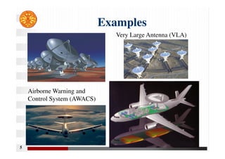
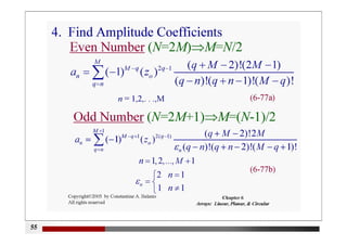
Examples
Very Large Antenna (VLA)
Airborne Warning and
Control System (AWACS)
6.
6
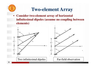
Two-element Array
• Considertwo-element array of horizontal
infinitesimal dipoles (assume no coupling between
elements)
Far-field observation
Two infinitesimal dipoles
7.
7
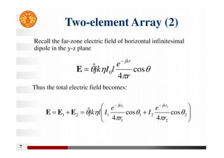
Two-element Array (2)
cos
4
ˆ
0
r
e
l
I
jk
jkr
E
Recall the far-zone electric field of horizontal infinitesimal
dipole in the y-z plane
2
2
2
1
1
1
2
1 cos
4
cos
4
ˆ
2
1
r
e
I
r
e
I
l
jk
jkr
jkr
E
E
E
Thus the total electric field becomes:
8.
8
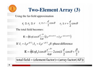
Two-Element Array (3)
cos
2
1
d
r
r
cos
2
2
d
r
r
r
r
r
2
1
Using the far-field approximation
2
/
cos
2
2
/
cos
1
4
cos
ˆ
jkd
jkd
jkr
e
I
e
I
r
e
l
jk
E
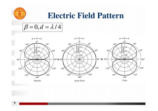
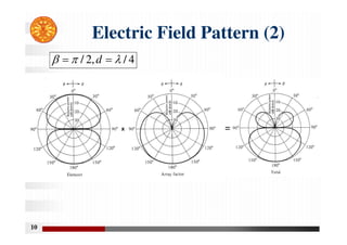
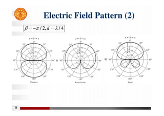
The total field becomes:
)
2
cos
2
cos(
2
4
cos
ˆ
0
d
k
r
e
l
I
jk
jkr
E
difference
phase
:
,
;
If 2
/
0
2
2
/
0
1
j
j
e
I
I
e
I
I
)
factor(AF)
(array
factor)
(element
field
total
12
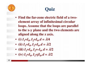
Quiz
• Find thefar-zone electric field of a two-
element array of infinitesimal circular
loops. Assume that the loops are parallel
to the x-y plane and the two elements are
aligned along the z axis.
• (i) I1=I0, I2=I0, d = λ
λ
λ
λ/4
• (ii) I1=I0, I2=I0, d = λ
λ
λ
λ/2
• (iii) I1=I0, I2=-I0, d = λ
λ
λ
λ/2
• (iv) I1=I0, I2=jI0, d = λ
λ
λ
λ/2
13.
13
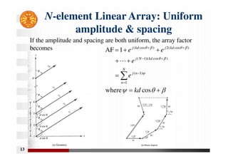
N-element Linear Array:Uniform
amplitude & spacing
cos
where
1
AF
1
)
1
(
)
cos
)(
1
(
)
cos
(
2
)
cos
(
kd
e
e
e
e
N
n
n
j
kd
N
j
kd
j
kd
j
L
If the amplitude and spacing are both uniform, the array factor
becomes
14.
14
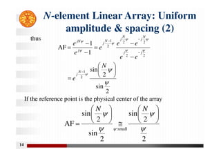
N-element Linear Array:Uniform
amplitude & spacing (2)
2
sin
2
sin
1
1
AF
2
1
2
2
2
2
2
1
N
e
e
e
e
e
e
e
e
N
j
j
j
N
j
N
j
N
j
j
jN
thus
If the reference point is the physical center of the array
2
2
sin
2
sin
2
sin
AF
small
:
N
N
15.
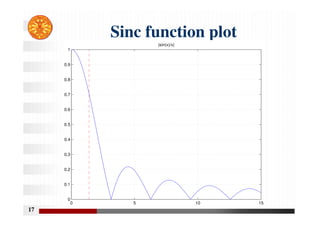
15
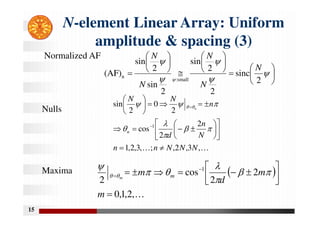
N-element Linear Array:Uniform
amplitude & spacing (3)
2
sinc
2
2
sin
2
sin
2
sin
(AF)
small
:
n
N
N
N
N
N
K
K ,
3
,
2
,
;
,
3
,
2
,
1
2
2
cos
2
0
2
sin
1
N
N
N
n
n
N
n
d
n
N
N
n
n
Normalized AF
Nulls
K
,
2
,
1
,
0
2
2
cos
2
1
m
m
d
m m
m
Maxima
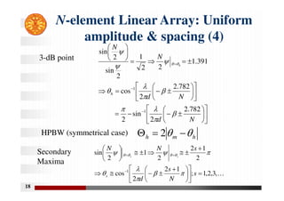
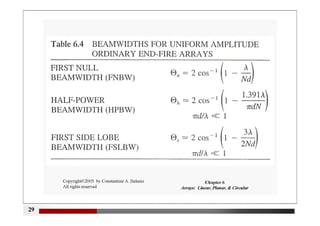
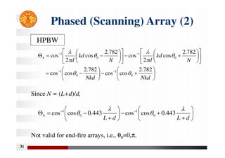
18
N-element Linear Array:Uniform
amplitude & spacing (4)
N
d
N
d
N
N
h
h
782
.
2
2
sin
2
782
.
2
2
cos
391
.
1
2
2
1
2
sin
2
sin
1
1
HPBW (symmetrical case)
3-dB point
Secondary
Maxima
h
m
h
2
K
,
3
,
2
,
1
;
1
2
2
cos
2
1
2
2
1
2
sin
1
s
N
s
d
s
N
N
s
s
s
19.
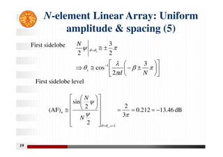
19
N-element Linear Array:Uniform
amplitude & spacing (5)
First sidelobe
N
d
N
s
s
3
2
cos
2
3
2
1
dB
46
.
13
212
.
0
3
2
2
2
sin
(AF)
1
,
n
s
s
N
N
First sidelobe level
20.
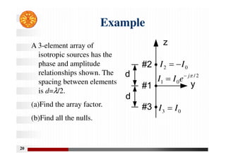
20
Example
#2
#1
#3
d
d
z
y
0
2 I
I
2
/
0
1
j
e
I
I
0
3 I
I
A 3-element array of
isotropic sources has the
phase and amplitude
relationships shown. The
spacing between elements
is d=λ/2.
(a)Find the array factor.
(b)Find all the nulls.
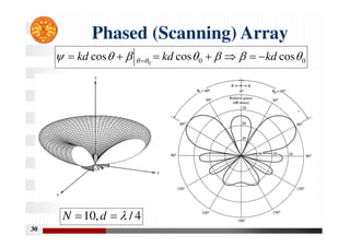
27
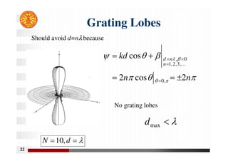
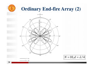
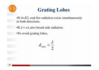
Grating Lobes
•If d=λ/2,end-fire radiation exists simultaneously
in both directions.
•If d = nλ, also broad-side radiation.
•To avoid grating lobes,
2
max
d
37
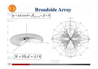
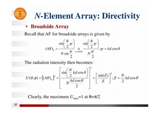
N-Element Array: Directivity
•Broadside Array
cos
;
2
2
sin
2
sin
2
sin
(AF)
small
:
n kd
N
N
N
N
cos
2
;
)
sin(
2
cos
cos
2
sin
)
AF
(
)
,
(
2
2
2
kd
N
Z
Z
Z
kd
N
kd
N
U n
Recall that AF for broadside arrays is given by
The radiation intensity then becomes:
Clearly, the maximum Umax=1 at θ=π/2
38.
38
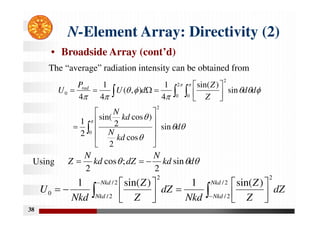
N-Element Array: Directivity(2)
• Broadside Array (cont’d)
The “average” radiation intensity can be obtained from
Using
0
2
2
0 0
2
0
sin
cos
2
)
cos
2
sin(
2
1
sin
)
sin(
4
1
)
,
(
4
1
4
d
kd
N
kd
N
d
d
Z
Z
d
U
P
U rad
d
kd
N
dZ
kd
N
Z sin
2
;
cos
2
2
/
2
/
2
/
2
/
2
2
0
)
sin(
1
)
sin(
1 Nkd
Nkd
Nkd
Nkd
dZ
Z
Z
Nkd
dZ
Z
Z
Nkd
U
39.
39
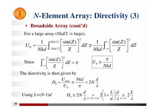
N-Element Array: Directivity(3)
• Broadside Array (cont’d)
dZ
Z
Z
Nkd
dZ
Z
Z
Nkd
U
Nkd
Nkd
2
2
/
2
/
2
0
)
sin(
1
)
sin(
1
For a large array (Nkd/2 -> large),
The directivity is then given by
d
N
Nkd
U
U
D 2
0
max
0
dZ
Z
Z
2
)
sin(
Nkd
U
0
L
d
d
L
d
N
D
d
L
d
N
L
2
1
2
2
)
1
(
0
Using L=(N-1)d
Since
40.
40
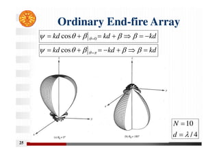
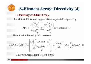
N-Element Array: Directivity(4)
• Ordinary end-fire Array
)
1
(cos
;
2
2
sin
2
sin
2
sin
(AF)
small
:
n
kd
N
N
N
N
)
1
(cos
2
;
)
sin(
2
)
1
(cos
)
1
(cos
2
sin
)
AF
(
)
,
(
2
2
2
kd
N
Z
Z
Z
kd
N
kd
N
U n
Recall that AF for ordinary end-fire arrays (θ=0) is given by
The radiation intensity then becomes:
Clearly, the maximum Umax=1 at θ=0
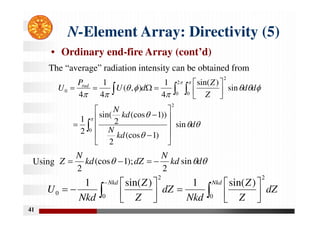
41.
41
N-Element Array: Directivity(5)
• Ordinary end-fire Array (cont’d)
The “average” radiation intensity can be obtained from
Using
0
2
2
0 0
2
0
sin
)
1
(cos
2
))
1
(cos
2
sin(
2
1
sin
)
sin(
4
1
)
,
(
4
1
4
d
kd
N
kd
N
d
d
Z
Z
d
U
P
U rad
d
kd
N
dZ
kd
N
Z sin
2
);
1
(cos
2
Nkd Nkd
dZ
Z
Z
Nkd
dZ
Z
Z
Nkd
U
0 0
2
2
0
)
sin(
1
)
sin(
1
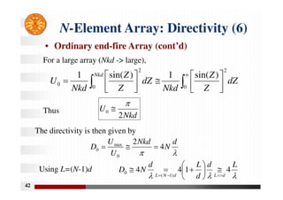
42.
42
N-Element Array: Directivity(6)
• Ordinary end-fire Array (cont’d)
0
2
0
2
0
)
sin(
1
)
sin(
1
dZ
Z
Z
Nkd
dZ
Z
Z
Nkd
U
Nkd
For a large array (Nkd -> large),
The directivity is then given by
d
N
Nkd
U
U
D 4
2
0
max
0
Nkd
U
2
0
L
d
d
L
d
N
D
d
L
d
N
L
4
1
4
4
)
1
(
0
Using L=(N-1)d
Thus
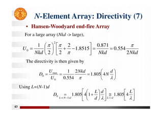
43.
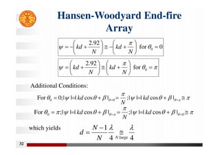
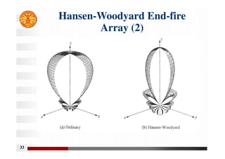
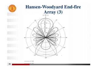
43
N-Element Array: Directivity(7)
• Hansen-Woodyard end-fire Array
Nkd
Nkd
Nkd
U
2
554
.
0
871
.
0
8515
.
1
2
2
2
1
2
0
For a large array (Nkd -> large),
The directivity is then given by
d
N
Nkd
U
U
D 4
805
.
1
2
554
.
0
1
0
max
0
L
d
d
L
D
d
L
d
N
L
4
805
.
1
1
4
805
.
1
)
1
(
0
Using L=(N-1)d
45
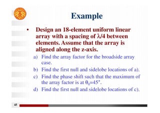
Example
• Design an18-element uniform linear
array with a spacing of λ
λ
λ
λ/4 between
elements. Assume that the array is
aligned along the z-axis.
a) Find the array factor for the broadside array
case.
b) Find the first null and sidelobe locations of a).
c) Find the phase shift such that the maximum of
the array factor is at θ0=45°.
d) Find the first null and sidelobe locations of c).
48
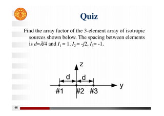
Quiz
Find the arrayfactor of the 3-element array of isotropic
sources shown below. The spacing between elements
is d=λ/4 and I1 = 1, I2 = -j2, I3= -1.
49.
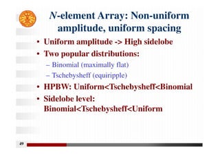
49
N-element Array: Non-uniform
amplitude,uniform spacing
• Uniform amplitude -> High sidelobe
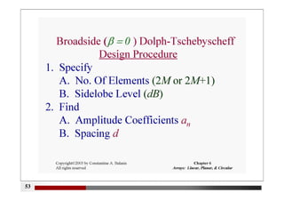
• Two popular distributions:
– Binomial (maximally flat)
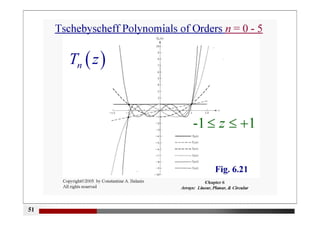
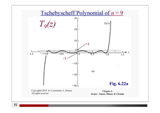
– Tschebysheff (equiripple)
• HPBW: Uniform<Tschebysheff<Binomial
• Sidelobe level:
Binomial<Tschebysheff<Uniform
59
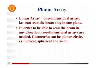
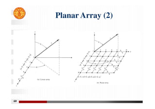
Planar Array
• LinearArray = one-dimensional array,
i.e., can scan the beam only in one plane.
• In order to be able to scan the beam in
any direction, two-dimensional arrays are
needed. Geometries can be planar, circle,
cylindrical, spherical and so on.

![46
18-element AF (broadside array)
0 20 40 60 80 100 120 140 160 180
−50
−45
−40
−35
−30
−25
−20
−15
−10
−5
0
θ [Degree]
|(AF)
n
|
[dB]
18−element array factor (Broadside scan](https://image.slidesharecdn.com/chapter6-250523185249-cb90496b/85/Chapter-Chapter-Chapter-Chapter-Chapter-6-pdf-46-320.jpg)
![47
18-element AF (scan array)
0 20 40 60 80 100 120 140 160 180
−50
−45
−40
−35
−30
−25
−20
−15
−10
−5
0
θ [Degree]
|(AF)
n
|
[dB]
18−element array factor](https://image.slidesharecdn.com/chapter6-250523185249-cb90496b/85/Chapter-Chapter-Chapter-Chapter-Chapter-6-pdf-47-320.jpg)


![3_Antenna Array [Modlue 4] (1).pdf](https://cdn.slidesharecdn.com/ss_thumbnails/3antennaarraymodlue41-220419112111-thumbnail.jpg?width=640&height=640&fit=bounds)


