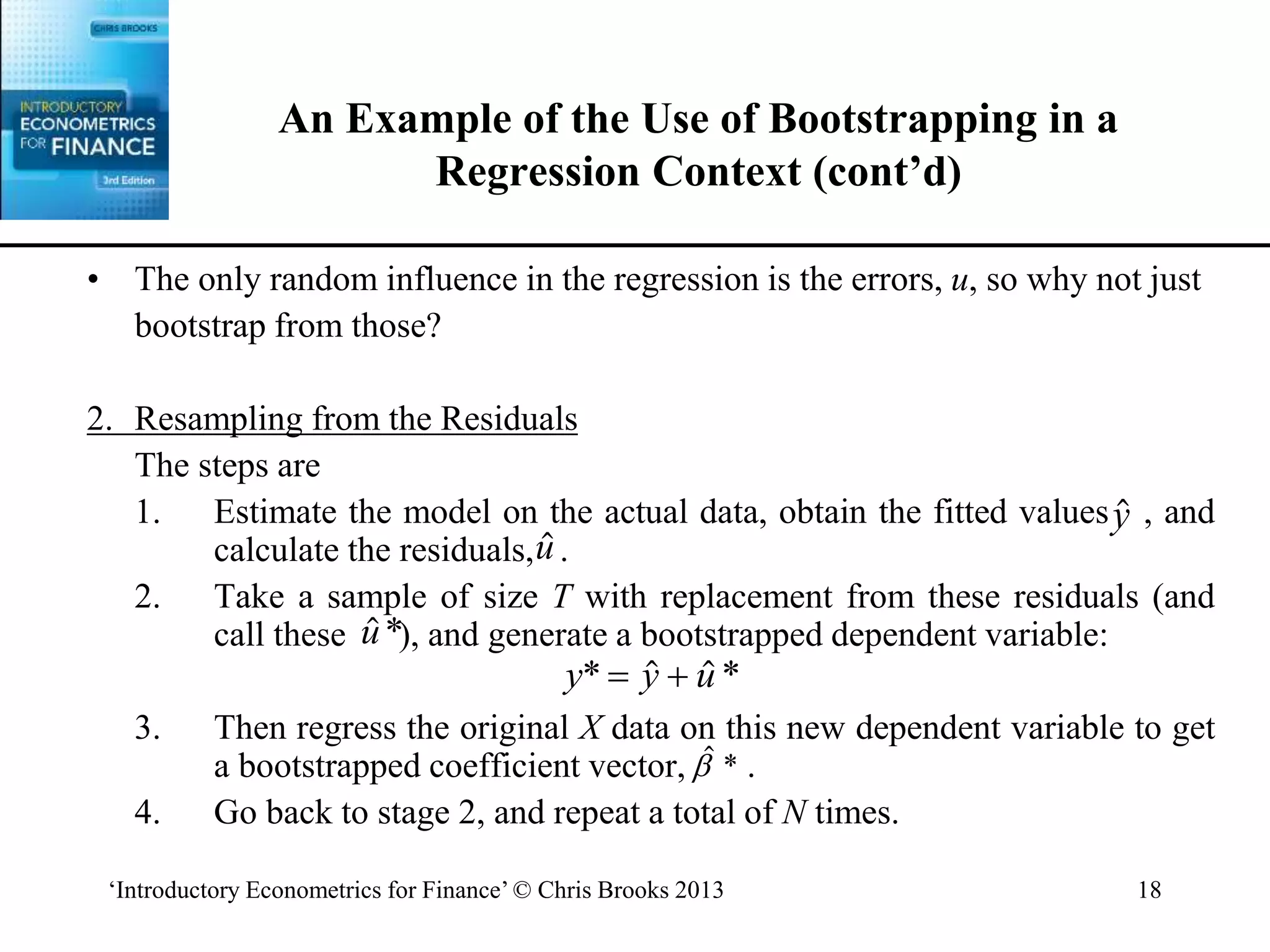
The document discusses simulation methods in econometrics and finance. It covers topics such as the Monte Carlo method, conducting simulation experiments by generating data and repeating experiments, random number generation, variance reduction techniques like antithetic variates and control variates, and examples of simulations in econometrics and finance including deriving critical values for Dickey-Fuller tests and pricing financial options. Bootstrapping methods are also discussed as an alternative to simulation that samples from real data rather than creating new data.
This document introduces the key concepts in econometrics and financial econometrics. It defines econometrics as the application of statistical and mathematical techniques to economic and financial problems. Some examples of problems that can be solved using econometrics are testing market efficiency, modeling volatility, and forecasting correlations. The document discusses the different types of data used in econometrics, including time series, cross-sectional, and panel data. It also covers important financial concepts like returns, deflating nominal values for inflation, and the differences between classical and Bayesian statistical approaches.
1. The document discusses switching models, which allow for changes in the behavior of economic and financial variables over time. These switches can be one-time changes or occur frequently.
2. Markov switching models generalize the dummy variable approach to allow for multiple "states of the world" that a variable can occupy. The probability of switching between states is governed by a transition probability matrix.
3. An example application uses a Markov switching model with two states to analyze real exchange rates. This allows for multiple switches between regimes and provides evidence on purchasing power parity theory.
This document discusses simultaneous equation models and issues that arise when estimating them. It introduces the concepts of structural and reduced form equations. Estimating structural equations individually using OLS will result in biased coefficients due to endogeneity. However, the reduced form equations can be estimated consistently using OLS as their right-hand side variables are exogenous. Identification issues may also arise if not enough information is present to separately estimate the structural parameters. Tests are discussed to check for exogeneity of variables.
1) The document introduces the multiple linear regression model, where the dependent variable depends on more than one independent variable. 2) It shows how to write the multiple regression model using a matrix formulation, with the dependent variable as a column vector, the independent variables as a matrix, and the coefficients and error term also as vectors/matrices. 3) It explains how to estimate the coefficients using ordinary least squares (OLS) and calculate the standard errors of the estimates.
This document discusses limited dependent variable models, where the dependent variable can only take on certain values, such as 0 or 1. It begins by providing examples of situations that would call for such models. It then examines the linear probability model and its flaws, such as producing probabilities outside the valid 0-1 range. Better approaches like the logit and probit models are discussed, which use functions to constrain probabilities to this range. The document also covers interpreting coefficients, goodness of fit measures, and estimating these models using maximum likelihood. As an application, it summarizes a study using a logit model to test theories of corporate financing decisions.
The document discusses panel data analysis and its application to analyzing competition in the UK banking sector. It summarizes:
1) Panel data has both time series and cross-sectional dimensions, allowing examination of how variables change over time for the same objects. A fixed effects model accounts for heterogeneity across objects.
2) A study analyzed competition in UK banking from 1980-2004 using a fixed effects panel data model. It tested for market equilibrium and calculated a contestability parameter to indicate the degree of competition.
3) The results found evidence of equilibrium and showed the contestability parameter fell from 0.78 to 0.46, suggesting competition weakened over the period.
This document provides an overview of how to conduct an event study in finance. It discusses why event studies are commonly used, how to define the event window and calculate abnormal returns, how to test hypotheses about the impact of events using standardized abnormal returns and cumulative abnormal returns, and how to average returns across firms and time periods. It also covers potential issues like cross-sectional dependence between firms' returns and changing return variances over the event window.
1) The document introduces the classical linear regression model, which describes the relationship between a dependent variable (y) and one or more independent variables (x). Regression analysis aims to evaluate this relationship.
2) Ordinary least squares (OLS) regression finds the linear combination of variables that best predicts the dependent variable. It minimizes the sum of the squared residuals, or vertical distances between the actual and predicted dependent variable values.
3) The OLS estimator provides formulas for calculating the estimated intercept (α) and slope (β) coefficients based on the sample data. These describe the estimated linear regression line relating y and x.
This document provides an overview of mathematical and statistical foundations relevant to econometrics. It defines functions and their linear and nonlinear forms. It discusses straight lines, their slopes and intercepts. It also covers quadratic functions, their roots and shapes. Additionally, it introduces exponential functions, logarithms, and their properties. It describes summation and differentiation notation used in calculus. The overall summary is an introduction to functions, lines, and other mathematical concepts important for understanding econometrics.
This document discusses the assumptions of the classical linear regression model (CLRM) and methods for testing violations of those assumptions. It covers the assumptions of no autocorrelation between error terms, homoscedasticity or constant error variance, and the errors being normally distributed. Tests for heteroscedasticity discussed include the Goldfeld-Quandt test and White's test. Tests for autocorrelation examined are the Durbin-Watson test and Breusch-Godfrey test. Consequences of violations include inefficient coefficient estimates and invalid inference. Potential remedies discussed are generalized least squares or using heteroscedasticity-robust standard errors.
The document discusses nonlinear models for volatility and correlation in financial data. It introduces the autoregressive conditional heteroscedasticity (ARCH) model and generalized ARCH (GARCH) models, which allow the variance of errors to depend on previous values. The ARCH model specifies the variance as a function of past squared errors. The GARCH model extends this to include the past variance, addressing issues with the ARCH model like how to determine the order q. Tests for ARCH effects and specifications of ARCH and GARCH models are also provided.
This document provides an overview of univariate time series modeling and forecasting. It defines concepts such as stationary and non-stationary processes. It describes autoregressive (AR) and moving average (MA) models, including their properties and estimation. It also discusses testing for autocorrelation and stationarity. The key models covered are AR(p) where the current value depends on p past lags, and MA(q) where the error term depends on q past error terms. Wold's decomposition theorem states that any stationary time series can be represented as the sum of deterministic and stochastic components.
This document discusses testing for non-stationarity and unit roots in time series data. It introduces the Augmented Dickey-Fuller (ADF) test and Phillips-Perron test for determining if a time series is integrated of order zero (I(0)), one (I(1)), or two (I(2)). The ADF test regressions the change in a variable on its lag and lags of the change to test for a unit root. If the null of a unit root is not rejected, further tests are needed to determine higher orders of integration. While ADF and Phillips-Perron tests are commonly used, their power is low if the process is near but not at the non-station
This document discusses various mathematical models used in finance to model stock prices and returns. It introduces random walk models, the lognormal model, general equilibrium theories, the Capital Asset Pricing Model (CAPM), and the Arbitrage Pricing Theory (ATP). The CAPM and ATP are equilibrium asset pricing models based on assumptions like rational investors seeking to maximize returns while minimizing risk.
This document provides an overview of key concepts for decision making under risk and uncertainty, including random variables, probability distributions, sampling, and Monte Carlo simulation. It introduces the concepts and outlines the steps for modeling problems that involve uncertain parameters through simulation. The goal is to simulate potential outcomes and evaluate alternatives while accounting for variation in inputs.
This document outlines the course content for Business Mathematics GMB 105 taught by Victor Gumbo from 28 August to 6 September 2014. It covers topics such as descriptive and inferential statistics, sampling methods, data accuracy and bias, frequency distributions, histograms, measures of central tendency and dispersion. Additional topics include compound interest, discounting, annuities, regression, correlation and dealing with multicollinearity in regression models. Examples are provided to illustrate key statistical and mathematical concepts.
This document discusses stationarity in time series analysis. It defines stationarity as a time series having a constant mean, constant variance, and constant autocorrelation structure over time. Non-stationary time series can be identified through run sequence plots, summary statistics, histograms, and augmented Dickey-Fuller tests. Common transformations like removing trends, heteroscedasticity through logging, differencing to remove autocorrelation, and removing seasonality can be used to make non-stationary time series data stationary. Python is used to demonstrate identifying and transforming non-stationary time series data.
Descriptive statistics helps users to describe and understand the features of a specific dataset, by providing short summaries and a graphic depiction of the measured data. Descriptive Statistical algorithms are sophisticated techniques that, within the confines of a self-serve analytical tool, can be simplified in a uniform, interactive environment to produce results that clearly illustrate answers and optimize decisions.
This document provides an overview of quantitative methods topics including time value of money, discounted cash flow applications, probability concepts, and statistical measures. Key points discussed include calculating present and future value of cash flows using timelines and interest rates, as well as methods for analyzing investments like net present value, internal rate of return, and holding period return. Common statistical concepts are also summarized such as measures of central tendency, frequency distributions, and histograms.
The document discusses cost-benefit analysis and various methods used to evaluate costs and benefits of projects. It defines key terms like tangible/intangible and direct/indirect costs and benefits. Several evaluation methods are described - net benefit analysis, present value analysis, net present value, payback period analysis, break-even analysis and cash flow analysis. Their formulas, examples and advantages/disadvantages are provided. The document concludes that cost-benefit analysis involves identifying, categorizing and evaluating costs and benefits to interpret results and take action regarding alternative systems.
This chapter discusses various methods for summarizing and exploring data, including dot plots, stem-and-leaf displays, percentiles, box plots, and scatter plots. Dot plots and stem-and-leaf displays organize data in a way that shows the distribution while maintaining each data point. Percentiles such as the median and quartiles divide data into equal portions. Box plots graphically show the center, spread, and outliers of data. Scatter plots reveal relationships between two variables, while contingency tables summarize categorical data relationships.
1. The document discusses demand estimation through regression analysis. Regression analysis uses empirical demand functions to estimate the relationship between a dependent variable (e.g. quantity demanded) and independent variables (e.g. price, income).
2. Simple and multiple regression analysis are explained. Simple regression uses one independent variable while multiple regression uses two or more. The Ordinary Least Squares method is commonly used to estimate coefficients.
3. The key steps in regression analysis are: specifying the model, estimating coefficients, interpreting results through statistical tests of significance, and using results for decision making like forecasting.
This document discusses various qualitative and quantitative forecasting methods including simple and weighted moving averages, exponential smoothing, and simple linear regression. It provides examples of how to calculate forecasts using each of these methods and evaluates forecast accuracy using metrics like MAD and tracking signal.
An ARIMAX model can be viewed as a multiple regression model with one or more autoregressive (AR) terms and/or one or more moving average (MA) terms. It is suitable for forecasting when data is stationary/non stationary, and multivariate with any type of data pattern, i.e., level/trend /seasonality/cyclicity. ARIMAX provides forecasted values of the target variables for user-specified time periods to illustrate results for planning, production, sales and other factors.
Beyond Classification and Ranking: Constrained Optimization of the ROInkaf61
This document summarizes a research paper that proposes a new learning algorithm to maximize return on investment (ROI) under budget constraints. The algorithm finds the subset of accounts that will have the highest total collection amount within the allowed pull rate. It does this by learning a differentiable objective function to approximate the ratio of monetary value to pull rate. On a credit card debt collection problem, the new algorithm achieved 11% higher average collection amount than weighted classification and ranking models.
Hierarchical Clustering is a process by which objects are classified into a number of groups so that they are as much dissimilar as possible from one group to another group and as similar as possible within each group. This technique can help an enterprise organize data into groups to identify similarities and, equally important, dissimilar groups and characteristics, so the business can target pricing, products, services, marketing messages and more.
This document discusses probability distributions in R. It defines probability distributions as ways to model real-life uncertain events and make inferences from sample data. It covers the binomial, Poisson, and normal distributions, and how to generate and analyze each using functions in R like dbinom(), rpois(), dnorm(), pnorm(), and qnorm(). These functions allow calculating probabilities, simulating distributions, and finding cutoff points for given probabilities.
Isotonic Regression is a statistical technique of fitting a free-form line to a sequence of observations such that the fitted line is non-decreasing (or non-increasing) everywhere, and lies as close to the observations as possible. Isotonic Regression is limited to predicting numeric output so the dependent variable must be numeric in nature…
This document provides an overview of simple and multiple linear regression analysis. It discusses key concepts such as:
- Dependent and independent variables in bivariate linear regression
- Using scatter plots to explore relationships
- Estimating regression coefficients and equations for simple and multiple regression models
- Using regression models to predict outcomes based on independent variable values
- Conducting statistical tests on overall regression models and individual coefficients
There are two types of random variables: discrete and continuous. A probability distribution can be viewed as a probability function or cumulative distribution function (CDF). Properties of these include being between 0 and 1 and the CDF non-decreasing. Binomial and Bernoulli distributions relate to binary outcomes. The normal distribution is widely used in portfolio theory and risk management. Monte Carlo simulation uses probability distributions to generate random samples for modeling complex financial systems.
In this Spark session Ravi Saraogi talks about why estimating default risk in fund structures can be a challenging task. He presents on how this process has evolved over the years and the current methodologies for assessing such risks.
Study on Application of Ensemble learning on Credit Scoringharmonylab
This document discusses using ensemble learning techniques for credit scoring applications. It begins by providing background on the growing need for effective credit scoring models due to the expansion of financing opportunities. It then discusses some common problems with credit scoring models, including a lack of understandability, multiple evaluation metrics, and imbalanced data. The purpose is to build a better credit scoring model using machine learning, specifically ensemble learning with XGBoost. Two proposed methods are described: 1) using EasyEnsemble resampling prior to XGBoost to address imbalanced data, and 2) customizing XGBoost by changing the evaluation metric to directly optimize cost or using a focal loss function. Experiments on several credit scoring datasets show these approaches can reduce costs without reducing accuracy
The document discusses nonlinear models for volatility and correlation in financial data. It introduces the autoregressive conditional heteroscedasticity (ARCH) model and generalized ARCH (GARCH) models, which allow the variance of errors to depend on previous values. Specifically, a GARCH(1,1) model is presented where the conditional variance is a function of the lagged squared errors and lagged variance. The document also discusses testing for ARCH effects and some limitations of ARCH models that GARCH addresses.
This document discusses different types of probability distributions including discrete and continuous distributions. It provides examples and formulas for binomial, Poisson, normal, and other distributions. It also includes sample problems demonstrating how to apply these distributions to real-world scenarios like fitting data to binomial or normal distributions and calculating probabilities based on Poisson or normal assumptions.
This document provides an overview of probabilistic models and their components. It discusses how probabilistic models incorporate random variables and probability distributions to account for uncertainty. Examples of probabilistic models covered include regression models, probability trees, Monte Carlo simulation, and Markov chains. The key building blocks - random variables and probability distributions - are explained. Special probability distributions like the Bernoulli, Binomial, and Normal distributions are also covered, along with summaries of distributions and the Empirical Rule.
Monte Carlo simulation is a computerized mathematical technique to
generate random sample data based on some known distribution for
numerical experiments.
• The Law of large numbers ensures that the relative frequency of
occurrence of a possible result of a random variable converges to the
theoretical or expected outcome as the number of experiments
increases.
• The essence of Monte Carlo simulation is to sample random variables
significant number of times so that the relative frequency converges to
the theoretical probability with greatest reliability
The document provides an overview of acquiring and processing time series data. It discusses analyzing energy consumption data from households to identify patterns and make predictions. Key steps include exploring and cleaning the data to handle issues like missing values, extracting relevant features, structuring the data for analysis in pandas, and techniques for handling missing data like imputation and converting between data formats. The goal is to efficiently analyze dynamic trends and relationships in the time series data.
This document discusses testing the normality assumption of log-returns for stock prices. It summarizes that the Black-Scholes model, widely used in pricing derivatives, assumes log-returns are normally distributed. The author tests this assumption on over 1000 company stock prices from the Nasdaq composite index using Kolmogorov-Smirnov, Shapiro-Wilk, and Anderson-Darling goodness-of-fit tests for normality with daily, weekly, and monthly price data from 2000-2011.
This document provides an overview of classical linear regression models. It defines regression analysis as describing the relationship between a dependent variable (y) and one or more independent variables (x). Ordinary least squares (OLS) regression fits a linear model to data by minimizing the sum of squared residuals. The OLS estimator for the slope coefficient β is derived. For the model to be estimated using OLS, it must be linear in parameters. The assumptions required for the classical linear regression model are listed.
Monte Carlo Simulations (UC Berkeley School of Information; July 11, 2019)Ivan Corneillet
My guest lecture on Monte Carlo simulations [or "how to be approximately right, now vs. precisely wrong, later (or never…)"] for the Managing Cyber Risk course of UC Berkeley School of Information's Cybersecurity Master.
This document discusses multiple regression analysis techniques. It begins by stating the goals of developing a statistical model to predict dependent variables from independent variables and using multiple regression when more than one independent variable is useful for prediction. It then provides an introduction to simple and multiple regression. The rest of the document discusses key aspects of multiple regression analysis, including linear models, the method of least squares, standard error of estimate, coefficient of multiple determination, hypothesis testing, and selection of predictor variables.
- The document outlines the steps for hypothesis testing including establishing null and alternative hypotheses, determining the appropriate statistical test, setting the significance level, establishing the decision rule, gathering and analyzing data, reaching a statistical conclusion, and making a business decision.
- It provides examples of hypothesis tests for a single mean when the population variance is known and unknown, including one-tailed and two-tailed tests. R code is given for working through hypothesis testing problems step-by-step in R.
This document provides an introduction to econometrics. It defines econometrics as the application of statistical and mathematical techniques to economic data in order to test economic theories and models. The document outlines the methodology of econometrics, including stating an economic theory, specifying mathematical and econometric models, obtaining data, estimating models, hypothesis testing, forecasting, and using models for policy purposes. It also discusses the structure of economic data such as time series, cross-sectional, and panel data. Finally, it covers key econometric concepts like the categories of variables and the differences between ratio and interval scales.
This document describes a bootstrap project analyzing population and sampling distributions using different bootstrap methods. It summarizes the general bootstrap method, bootstrap without replacement (BWO), and mirror-match approaches. Results show the bootstrap sampling distributions mimic the actual distributions and produce accurate estimates of statistics and variances. However, BWO and mirror-match had vastly greater processing times with no statistical advantage over the general bootstrap method for the stratified samples analyzed in this study.
This document discusses building technically sound simulation models in Crystal Ball. It covers:
- Common applications of simulation modeling and Crystal Ball software.
- The ModelAssist reference tool for simulation best practices.
- Key technical considerations like properly modeling multiplications as sums, distinguishing variability from uncertainty, and accounting for dependencies between variables.
- A checklist of best practices such as engaging decision-makers, keeping models simple, and clearly communicating results.
Andres hernandez ai_machine_learning_london_nov2017Andres Hernandez
My slides from the AI & Machine Learning in Quantitative Finance conference in London. I train a neural network to train another neural network to optimize particular black boxes
How to Implement a Strategy: Transform Your Strategy with BSC Designer's Comp...Aleksey Savkin
The Strategy Implementation System offers a structured approach to translating stakeholder needs into actionable strategies using high-level and low-level scorecards. It involves stakeholder analysis, strategy decomposition, adoption of strategic frameworks like Balanced Scorecard or OKR, and alignment of goals, initiatives, and KPIs.
Key Components:
- Stakeholder Analysis
- Strategy Decomposition
- Adoption of Business Frameworks
- Goal Setting
- Initiatives and Action Plans
- KPIs and Performance Metrics
- Learning and Adaptation
- Alignment and Cascading of Scorecards
Benefits:
- Systematic strategy formulation and execution.
- Framework flexibility and automation.
- Enhanced alignment and strategic focus across the organization.
Event Report - SAP Sapphire 2024 Orlando - lots of innovation and old challengesHolger Mueller
Holger Mueller of Constellation Research shares his key takeaways from SAP's Sapphire confernece, held in Orlando, June 3rd till 5th 2024, in the Orange Convention Center.
Brian Fitzsimmons on the Business Strategy and Content Flywheel of Barstool S...Neil Horowitz
On episode 272 of the Digital and Social Media Sports Podcast, Neil chatted with Brian Fitzsimmons, Director of Licensing and Business Development for Barstool Sports.
What follows is a collection of snippets from the podcast. To hear the full interview and more, check out the podcast on all podcast platforms and at www.dsmsports.net
[To download this presentation, visit:
https://www.oeconsulting.com.sg/training-presentations]
This PowerPoint compilation offers a comprehensive overview of 20 leading innovation management frameworks and methodologies, selected for their broad applicability across various industries and organizational contexts. These frameworks are valuable resources for a wide range of users, including business professionals, educators, and consultants.
Each framework is presented with visually engaging diagrams and templates, ensuring the content is both informative and appealing. While this compilation is thorough, please note that the slides are intended as supplementary resources and may not be sufficient for standalone instructional purposes.
This compilation is ideal for anyone looking to enhance their understanding of innovation management and drive meaningful change within their organization. Whether you aim to improve product development processes, enhance customer experiences, or drive digital transformation, these frameworks offer valuable insights and tools to help you achieve your goals.
INCLUDED FRAMEWORKS/MODELS:
1. Stanford’s Design Thinking
2. IDEO’s Human-Centered Design
3. Strategyzer’s Business Model Innovation
4. Lean Startup Methodology
5. Agile Innovation Framework
6. Doblin’s Ten Types of Innovation
7. McKinsey’s Three Horizons of Growth
8. Customer Journey Map
9. Christensen’s Disruptive Innovation Theory
10. Blue Ocean Strategy
11. Strategyn’s Jobs-To-Be-Done (JTBD) Framework with Job Map
12. Design Sprint Framework
13. The Double Diamond
14. Lean Six Sigma DMAIC
15. TRIZ Problem-Solving Framework
16. Edward de Bono’s Six Thinking Hats
17. Stage-Gate Model
18. Toyota’s Six Steps of Kaizen
19. Microsoft’s Digital Transformation Framework
20. Design for Six Sigma (DFSS)
To download this presentation, visit:
https://www.oeconsulting.com.sg/training-presentations
Taurus Zodiac Sign: Unveiling the Traits, Dates, and Horoscope Insights of th...my Pandit
Dive into the steadfast world of the Taurus Zodiac Sign. Discover the grounded, stable, and logical nature of Taurus individuals, and explore their key personality traits, important dates, and horoscope insights. Learn how the determination and patience of the Taurus sign make them the rock-steady achievers and anchors of the zodiac.
Industrial Tech SW: Category Renewal and CreationChristian Dahlen
Every industrial revolution has created a new set of categories and a new set of players.
Multiple new technologies have emerged, but Samsara and C3.ai are only two companies which have gone public so far.
Manufacturing startups constitute the largest pipeline share of unicorns and IPO candidates in the SF Bay Area, and software startups dominate in Germany.
Structural Design Process: Step-by-Step Guide for BuildingsChandresh Chudasama
The structural design process is explained: Follow our step-by-step guide to understand building design intricacies and ensure structural integrity. Learn how to build wonderful buildings with the help of our detailed information. Learn how to create structures with durability and reliability and also gain insights on ways of managing structures.
Company Valuation webinar series - Tuesday, 4 June 2024FelixPerez547899
This session provided an update as to the latest valuation data in the UK and then delved into a discussion on the upcoming election and the impacts on valuation. We finished, as always with a Q&A
The 10 Most Influential Leaders Guiding Corporate Evolution, 2024.pdfthesiliconleaders
In the recent edition, The 10 Most Influential Leaders Guiding Corporate Evolution, 2024, The Silicon Leaders magazine gladly features Dejan Štancer, President of the Global Chamber of Business Leaders (GCBL), along with other leaders.
How MJ Global Leads the Packaging Industry.pdfMJ Global
MJ Global's success in staying ahead of the curve in the packaging industry is a testament to its dedication to innovation, sustainability, and customer-centricity. By embracing technological advancements, leading in eco-friendly solutions, collaborating with industry leaders, and adapting to evolving consumer preferences, MJ Global continues to set new standards in the packaging sector.
Part 2 Deep Dive: Navigating the 2024 Slowdownjeffkluth1
Introduction
The global retail industry has weathered numerous storms, with the financial crisis of 2008 serving as a poignant reminder of the sector's resilience and adaptability. However, as we navigate the complex landscape of 2024, retailers face a unique set of challenges that demand innovative strategies and a fundamental shift in mindset. This white paper contrasts the impact of the 2008 recession on the retail sector with the current headwinds retailers are grappling with, while offering a comprehensive roadmap for success in this new paradigm.
3 Simple Steps To Buy Verified Payoneer Account In 2024SEOSMMEARTH
Buy Verified Payoneer Account: Quick and Secure Way to Receive Payments
Buy Verified Payoneer Account With 100% secure documents, [ USA, UK, CA ]. Are you looking for a reliable and safe way to receive payments online? Then you need buy verified Payoneer account ! Payoneer is a global payment platform that allows businesses and individuals to send and receive money in over 200 countries.
If You Want To More Information just Contact Now:
Skype: SEOSMMEARTH
Telegram: @seosmmearth
Gmail: seosmmearth@gmail.com
Discover timeless style with the 2022 Vintage Roman Numerals Men's Ring. Crafted from premium stainless steel, this 6mm wide ring embodies elegance and durability. Perfect as a gift, it seamlessly blends classic Roman numeral detailing with modern sophistication, making it an ideal accessory for any occasion.
https://rb.gy/usj1a2
Easily Verify Compliance and Security with Binance KYCAny kyc Account
Use our simple KYC verification guide to make sure your Binance account is safe and compliant. Discover the fundamentals, appreciate the significance of KYC, and trade on one of the biggest cryptocurrency exchanges with confidence.
❼❷⓿❺❻❷❽❷❼❽ Dpboss Matka Result Satta Matka Guessing Satta Fix jodi Kalyan Final ank Satta Matka Dpbos Final ank Satta Matta Matka 143 Kalyan Matka Guessing Final Matka Final ank Today Matka 420 Satta Batta Satta 143 Kalyan Chart Main Bazar Chart vip Matka Guessing Dpboss 143 Guessing Kalyan night
Best practices for project execution and deliveryCLIVE MINCHIN
A select set of project management best practices to keep your project on-track, on-cost and aligned to scope. Many firms have don't have the necessary skills, diligence, methods and oversight of their projects; this leads to slippage, higher costs and longer timeframes. Often firms have a history of projects that simply failed to move the needle. These best practices will help your firm avoid these pitfalls but they require fortitude to apply.