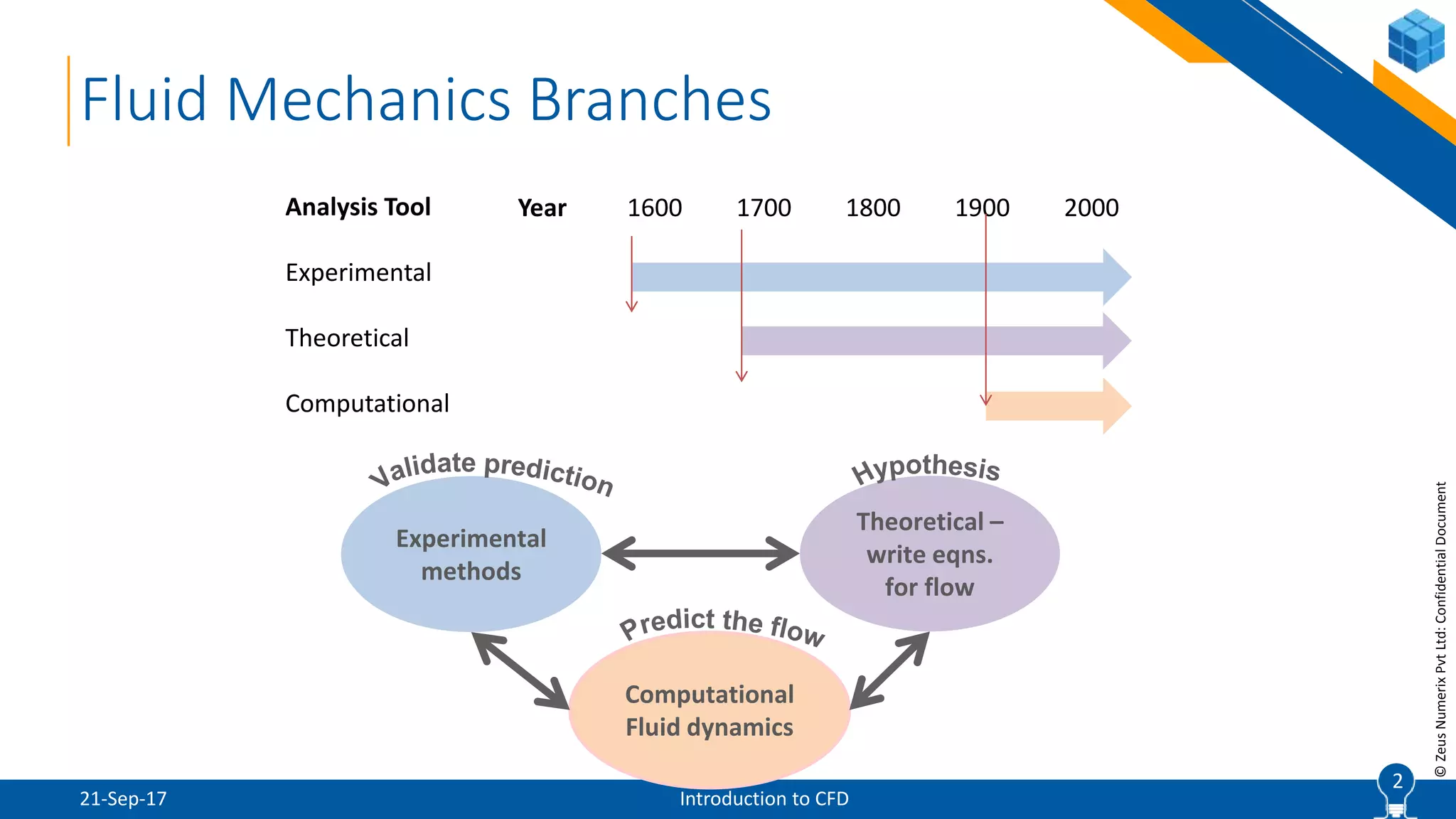
CFD Lecture (2/8): Fluid Mechanics: CFD Perspective

1Built-to-Spec | Product Approval | Engineering Services | Software Development
Fluid Mechanics: CFD Perspective
Fluid mechanics primer (initial thoughts) for CFD
and equations of CFD and uses
 Prof Anil W Date
 Mechanical Engineering, IIT Bombay

2
©ZeusNumerixPvtLtd:ConfidentialDocument
21-Sep-17 Introduction to CFD
2
Fluid Mechanics Branches
Theoretical –
write eqns.
for flow
Experimental
methods
Computational
Fluid dynamics
Analysis Tool
Experimental
Theoretical
Computational
Year 1600 1700 1800 1900 2000

3
Theoretical Fluid Dynamics (TFD)
 Most important branch of fluid dynamics
 Crucial in understanding concepts (e.g. Lift = ρUxΓ)
 Compressible flow in a converging diverging nozzles
 Usually good in predicting trends (e.g.: δ ~ Re-1/2)
 Generates ample information with simple assumptions
 SR-71 Blackbird designed completely using TFD
 TFD requires insight
 Requires extensive training/experience
 Idea to incorporate most fluid dynamics in tools
 Manual work requires knowledge of essential fluid dynamics
3

4
What Should I Learn?
 Everyone MUST learn theoretical fluid dynamics
 A good engineer should understand the pro’s and con’s of computational vs.
experimental methods
 Interestingly in old days
 Everyone believed experimental results except the person who conducted the
experiment
 No one believed results from Computational Fluid Dynamics except the person who did
CFD
 What made this difference?
 Computing power and algorithms to resolve the scales turbulence (i.e. essence of fluid
flow)
4

5
5
Computing Power: Flow over Wing
Method
Scale of
turbulence
Resolution required
Surface
points
Wake points Time steps
Total
operations
Direct Navier Stokes
(DNS)
No modeling 1016 1017 108 1025
Large Eddy Simulation
(LES)
Sub-grid modeling 1012 109 108 1020
LES with wall layer
Near wall & sub-
grid modeling
1010 109 107 1017
Reynolds Navier Stokes
(RANS)
All scales are
modeled
107 107 104 1011
Euler equation Scales are absent 107 107 103 1010
Inviscid vortex based
methods
Scales are absent 102 102 103 105
WingofAR=10,Re=5x106

6
Physics of Flow
Mathematical formulations
6

7
Physics of Incompressible Flow
 Incompressible flow is governed by:
 Conservation of mass (continuity equation)
u/x + v/y + w/z = 0 (1)
 Conservation of momentum (Euler equation)
(u/t + uu/x + vu/y + wu/z) + p/x = 0 (2)
( v/t + uv/x + vv/y + wv/z )+ p/y = 0 (3)
 (w/t + uw/x + vw/y + ww/z) + p/z = 0 (4)
 Density is constant. Temperature doesn’t take part in motion of flow
 Heat energy of an element, e or temperature, T (if Cp is constant) is convected as if
‘T’ is an independent attribute of fluid not related to its motion
7

8
Physics of Incompressible Flow
 In incompressible flows, kinetic energy may convert to internal energy (heat), but not
vice versa
 Specific heat capacity of liquids large
 Insignificant effect on temperature due to loss of kinetic energy
 Thus only four equations (accounting for viscosity) are adequate for solution of
incompressible fluid motion .
 The energy equation is required to be coupled with eqn of motion. It would be in fact
wrong to simultaneously solve for them
8

9
Peculiarity of PDEs
 In principle eqns. (2) to (4) ( slide 7)can be used to correct u, v and w from their
guesses (initial condition)
 What can be done so that pressure can be corrected from its initial condition ? Note
that a term p/t does not exist.
 Mathematically, treatment for p must be different from the treatment to be given to
u, v and w
 Interestingly, p/ x, p/ y and p/ z appear in the equations, but pressure, p does
not appear in any of the equations. Thus the solution does not change if p = p +
constant
9

10
Compressible Flow
 Compressible flow is governed by:
 Conservation of mass (continuity equation)
/t + (u)/x + (v)/y + (w)/z = 0 (1)
 Conservation of momentum (Euler equation)
(u)/t + (u2)/x + (uv)/y + (uw)/z + p/x = 0 (2)
(v)/t + (uv)/x + (v2)/y + (vw)/z + p/y =0 (3)
(w)/t + (uw)/x + (vw)/y + (w2)/z + p/z = 0 (4)
 Conservation of energy equation
(E)/t + (u(E+p))/x + (v(E+p))/y + (w(E+p))/z = 0 (5)
10

11
Physics of Compressible Flow
E =  (e + ½ u2)
E = internal energy (e) + kinetic energy (½ u2)
 In principle eqns. (1) to (5) can be used to correct ρ, u, v, w and E (or e) from their
initial condition
 What can be done so that pressure can be corrected from its initial condition? Note
that there is no equation for p. This is where equation of state (EoS) can be used
p = (-1)(E- ½ u2)
 Note that equations do have p as well as p/ x, p/ y and p/ z. Hence solution
depends on pressure, p
11

12
Peculiarity of PDEs
 There 6 unknown (ρ, u, v, w, e and p) and 5 partial differential equations + one
algebraic equations; i.e. the problem is well posed.
 Interestingly, compressible CFD prefers to choose internal energy, e as a variable and
hence equation of state is p =ρ (γ-1)(E- ½ u2) and not the conventional p = ρRT
 In compressible flows, internal energy can be converted to mechanical and kinetic
energy and vice versa. Thus momentum equation can not be considered as
conservation of momentum equation.
 Though not stated explicitly, the second law of thermodynamics must be obeyed
12

13
CFD the Tool
Description of CFD Process
13

14
14
CFD in Six Steps
3
2
Build Computational
Domain
Create
suitable Mesh
Boundary Conditions &
Initial conditions
Solution of discrete equationsPlot flow FieldInterpret solution
These steps will be discussed in detail in this workshop

15
Brief Steps
 Identify the computational domain
 Generate the correct type of mesh
 Structured or Unstructured mesh or hybrid mesh
 Set up Simulation
 Assign boundary conditions, initial conditions, etc
 Execute the solver
 Choose accuracy, Viscous/In-viscid, Laminar / Turbulent, Incompressible / compressible,
etc
 Post-process the data
 Organize data and understand results
15

16
Brief Steps
20-May-2019 Capabilities on Land Systems @ Zeus Numerix
 Understand the fluid dynamics
 Do the results make any sense? Is the design correct?
 Note that at every step, good understanding of theoretical fluid dynamics is
essential!
16

17
CFD – The Computational Tool
 CFD tools are required for solving industrial problems
 Emphasis is on economy of solution without sacrificing the required accuracy
 Advances are in tools is linked to other branches of technology; e.g. storage devices
 Tools are for getting rid of manual work
 Tools must capture as much physics as possible from first principle
 They must a part of larger suite of simulation technologies such as FEM, CEM, etc.
being used by the engineering fraternity
 Measure of success – the ease with which diverse problems can be solved
17

18
Four important Tools of CFD
 Importance of the tools vis-à-vis time
 Creating / Repairing Geometry
 Discretising Domain
 Numerical Simulation
 Post-processing the Data
18
0
10
20
30
40
50
60
70
80
Days
CAD Grids Solution Post_processing
0
1
2
3
4
5
6
7
Days
0
20
40
60
80
100
120
140
160
180
Minutes
Case #2
Case #3
Case #1
Source : Catherine M. Maskyumiuk, et. al.
Application of CFD in Aeronautics at
NASAAMES Research Centre, pp 57-67,
NASA CP 3291, 1995

19
CAD Geometry
 Importance of Geometry in CFD
 CFD tools can become a commodity only if CAD data is read
 Geometry fidelity is an essential element in CFD, Retain the details that matter for
simulation
 Errors in CAD data in the form of gaps, overlaps, non-physical protrusions is expensive
19

20
 Structured Grids - One-to-one
mapping
 Sponge analogy: Transform a 2D
domain in to a rectangle (and 3D
domain to a box) by a suitable affine
transformation
 How to divide the domain into
collection of rectangular blocks?
 Un-structured Grids
 Assembly of simple shapes : Fill a
given domain with simple shapes
such as triangles so that given
domain is fully covered
 Emphasis is on cells there are grid
points but no continuous lines or
what can be called as grid lines
20
Grid Generation

21
0
10
20
30
40
50
60
70
80
0thdimension
1D
Axisymmetric
2DSingleBody
2DUnsteady
2DMulti-Body
3DSingleBody
3DMulti-Body
Numerical Algorithms
 3D Problems are very complex to solve, 2D constitutes CFD of one year duration
 Reactive flows bigger challenge than viscosity
 Modelling turbulence & phase change are research fields
21
Normally taught in universities

22
Post-Processing
 Purpose of computing in insight; not only no’s
 Advection of massless particle from one point to another obeys two differential
equation
Position = Position |t =0 + (t) velocity
D(colour)/Dt = C 2(color concentration)
22

23
Universal Challenge
 Reduce Development Cost
 Current design methods: more than 70 % of project cost goes for Test-Fail-Fix cycle
 Can we carry out “Test-Fail-Fix cycle” with virtual parts, sub-systems, systems?
23
Where We Need to be

24
CFD; An Enabling Technology
 The Technology Readiness Level (TRL) of CFD has moved from TRL 1 to TRL 7
 The current Requirements
 CFD now works for “real” problems
 CFD is an engineering tool for designers and NOT ONLY for CFD scientist
 Turnaround times is compatible with the design cycle (say)
 Conceptual design (1-2 months)
 Preliminary design (4-6 months)
 Detail design (6-9 months)
 It must produce required accuracy
 The cost must be reasonable
24

25
CFD: Design Process
 CFD needs provide
 Flow field analysis
 Structural and thermal loads
 Approach - Use best tool available
 Use Multiple customized tools
 Get solutions from many software developed strategic partners, in-house, commercial
of-the-shelf, or government laboratories
 Always use hierarchical physical models (e.g. laminar flames first then turbulent flames)
 Validate and calibrate periodically
 Emphasize getting engineering solutions and not very accurate solution
 CFD results must make physical sense
25

26
Validation
 Validation is essential
 Ensure that analysis results are sufficiently reliable and accurate for intended purposes
 Must Provide necessary confidence to the designer
 It should offer to quantify
 Code accuracy and sensitivities
 Validation is learning process for application engineers
 Important to know what not to do
 Validation process depend on end application and the intended use of CFD
26

27
Current Status
 Now CFD is defined as a process of understanding flow field
 Most time consuming process are
 CAD repair and
 Mesh generation
 Automating the CAD repair and mesh generation will lead to high efficiency
 Current problems size is around 20 to 30 million cells. Complete aircraft, missile,
rocket, etc can be analysed
 Turn around time for a drag polar on high performance computers could be less than
12 hours
27

28
CFD Needs
 Extensive use of CFD requires quality data for validation. The quality data sources
are:
 Analytical solutions
 Very high fidelity simulations (e.g. DNS)
 Benchmark experiments
 Subcomponent Component tests and system tests
 Validation is industry specific
 Validation for aerospace applications can not be derived from automobile industry
 Validation is continuous process
28

29
References
 Introduction to Computational Fluid Dynamics, A.W. Date, Cambridge
 Computational Fluid Dynamics, Anderson, JD, McGraw Hill
 An introduction to CFD, W. Malasekara, H. K. Versteeg
 Computational Methods for Fluid Dynamics, J. H. Ferziger & M. Peric, Spinger
 Computational Gas Dynamics, Cubert B. Laney, Cambridge university Press
 Handbook of Computational Fluid Mechanics, Roger Peyret
 Numerical Computation of Internal and External Flows (2 volumes), C. Hirsch, John
Wiley & Sons
29

30
References
20-May-2019 Capabilities on Land Systems @ Zeus Numerix
 Numerical Simulation in Fluid Dynamics – A practical Introduction, Michael Griebel,
et.al., Siam
 Numerical Methods for Conservation Laws, RJ Le Veque, Birkhauser Verlag
 Principles of Computational Fluid Dynamics, Pieter Wesseling, Spinger
 Riemann Solvers and Numerical Methods for Fluid Dynamics, Toro, E.F., Springer
30

31
www.zeusnumerix.com
+91 98190 09836
Abhishek Jain
abhishek@zeusnumerix.com

CFD Lecture (2/8): Fluid Mechanics: CFD Perspective

More Related Content

Similar to CFD Lecture (2/8): Fluid Mechanics: CFD Perspective

More from Abhishek Jain

Recently uploaded

CFD Lecture (2/8): Fluid Mechanics: CFD Perspective