![Proceedings of ICEAE 2009
Email addresses:
bharat.agrawal@zeusnumerix.com (Agrawal, B.R.)
saurabh.pandey@zeusnumerix.com (Pandey, S.)
1Corresponding Authors
1. INTRODUCTION
Grid generation is a crucial first step in the whole process
of numerically simulating a physics problem. Currently
structured and unstructured meshes are widely used in the
industry applications. However, they have the limitation that
they cannot be automatically generated over complex
geometries thus requiring large number of man hours in
manually creating these grids. This arise a need for an
automatic grid generation process. [1][2] Hereby, software
has been developed which can automatically generate an oct-
tree based Cartesian mesh over geometries of any
complexity. The code has been tested on various geometries
and is capable of generating 10 million cells in 10 seconds
on a serial machine. To begin the process of writing a
complex solver on these meshes an incompressible Euler
solver has been written. The solver so far is tested for very
simple standard test cases. The results over these meshes are
also discussed in the later sections.
2. Background and Motivation
Computational Fluid Dynamics is the field of numerical
equations approximately requires the use of computers to
solve any engineering problem. The advancements in
computer technology since 1970 have made it possible to
use it to do large amount of computation in a small amount
of time [1].
But this was regarding solution of PDEs, grid generation
part in CFD still lagged behind requiring a lot of human
involvement, therefore it was a time consuming process.
This produced the need of a quick and automatic grid
generation algorithm with minimal human involvement.
Cartesian meshes were introduced to cater to this increasing
demand of quick mesh generation generator [3][4].
Cartesian Mesh was good for low fidelity simulation but
if the desired accuracy of the solution was high the number
of cells in the grid increased drastically as there is no
concept of clustering in such mesh. Hence Oct-tree based
Cartesian Grid was developed. These grids have the
advantage of clustering and that too adaptive. If the gradient
in a cell is going beyond a threshold the cell can be divided
into eight equal cells to capture the gradient correctly
[3][5][6].
Oct-tree based Cartesian grid is also very advantageous
when the geometry of the body is very complex. If there is a
sharp corner or irregularities in the surface, it is very
difficult to capture the geometry using fixed size cells. But
using adaptive oct-tree grids the cells can be refined to a
very high level i.e. very small volume at places where very
small size cells are required to capture the geometry. This
Revisiting Projection Methods over Automatic Oct-tree Meshes
Agrawal, Bharat R. a,1
, Pandey, Saurabha
a
Zeus Numerix Pvt. Ltd., Mumbai
Abstract: This work documents the ongoing effort on using projection methods over automatic
oct-tree meshes. The mesh generation algorithm uses a quick and automatic method to create
solver and geometry adaptive oct-tree mesh on a basic Cartesian grid. The mesh is a non-body
fitted type of mesh and therefore is independent of the topology of the geometry. The method
takes multiple water tight triangulated surface(s) as an input. The software then automatically
creates oct-tree based Cartesian grids both outside as well as inside the geometry. The
intersection of the cells with the triangles of the geometry is done using a very robust and
efficient polygon clipping algorithm allowing the capture of geometry with 100% accuracy.
Over this mesh an incompressible Euler solver based on projection method is being written. The
solver is tested working for some simple test cases.
Key words: Projection Method, Oct-tree, Cartesian Mesh, Incompressible Euler](https://image.slidesharecdn.com/research-paper-revisiting-projection-methods-over-automatic-oct-tree-meshes-201118092705/75/Revisiting-Projection-Methods-over-Automatic-Oct-tree-Meshes-1-2048.jpg)
![ICEAE Paper GN-053
Proceedings of ICEAE 2009
improvement in capturing the geometry in turn improves the
accuracy of the solver [1].
These advantages of oct-tree grids over Cartesian grids
have a lot of promise in correctly simulating flow around
very complex geometries. As these grid can be generated in
no time over very complex geometries, if coupled with a
quick compressible or incompressible solver can used as a
design tool. Therefore oct-tree grid can be used to bring in
the utilization of CFD in designing phase [1][4].
3. Geometry Input
The software is aimed at reading geometries of any
complexities and which can be easily generated using CAD
software. There are various formats in which the CAD
software can save the geometry, however, triangulated
surfaces provides the best robustness required by a meshing
algorithm. The robustness parameter considered here is
primarily the water tightness of the geometry. The water
tight requirement arises from a function (further referred as
'inout function') which determines whether a point is outside
or inside the geometry. Further, the software can take
polygon surface also which is converted internally into a
triangulated surface by the software. The software can also
take multiple geometries as well which may or may not
intersect in the space.
Geometry is stored in a half edge data structure wherein
each edge is stored as a twin edge, each of these twin edges
are same edges with opposite direction. Each edge belongs
to two different adjacent triangles. This data structure
provides an excellent and efficient traversal over the edges
and vertices of all triangles and also their respective
neighbouring triangles.
4 Grid Data Structure
An oct-tree data structure has been used to store each cell
where each cell can have none or 8 children. The cells which
do not have children are the real existing cells of the grid
which will be used in the solver whereas the cells which
have children exist only for the completeness of the grid.
The data structure is designed in such a manner where any
neighbouring entity of a particular cell can be directly
accessed. Also, for a particular face the cells which share
that face can be directly accessed as right or left cell of that
face [1].
The data structure allows an object of class cell cut info,
face cut info and edge cut info to be associated with the cell,
face and edge respectively. Each of these cut info objects
stores the interaction of the cell with the geometry. Cell cut
info stores the surface polygons lying inside the cells, face
cut info stores the edges of these surface polygons which
completely lie in the faces and edge cut info stores the points
at which the edge is intersecting the geometry
5 Solver Requirements
5.1 Volume accuracy
First requirement is the accurate computation of the
volumes of all the cells in the computation domain. The
degree of accuracy in calculating the volumes of the cells
directly dictates the fidelity of the solution [3][5][6]. A large
number of cells in the oct-tree Cartesian mesh are regular
cuboids in shape. These regular cells have well defined plane
boundaries where the planes are x=const, y=const and
z=const. However, some of the cells which intersect with the
geometry can be chopped in any manner which creates
complicated polyhedron. Hence it is these cells whose
volume calculation requires computation effort and finally
dictating the solution fidelity.
5.2 Neighbour traversal
Second crucial requirement is the quick access to the
neighbouring entities of a cell such as neighbouring cells and
faces. This is taken care by the design of data structure
wherein each cell has pointers to its six faces and each face
has pointers to its left and right cells [1].
5.3 Level difference in adjacent cells
There is one constraint to ensure first order accuracy
while calculating gradients on the face. It is that the levels of
cells sharing a face, an edge or a vertex cannot differ by
more than one. In Fig. 1, the dotted lines are the refinement
happening because of this constraint [7].
5.4 Boundary carpet
Other constraint is to provide a layer of smooth equal
level cells over the whole geometry to ensure there is no
cells which have level less than the defined boundary level
(BL) very close to the boundary. This case arises when a cut
cell is very small in volume and since the adjacent cell is not
cutting the boundary it can remain at a lower level as
compared to the boundary level. This is done by making sure
each of the cells which are a candidate for being a cut cell
has all neighbours having level equal to that cell. The carpet
provides a smooth layer in which the boundary layer effects
Figure 1 Division of cells due to neighbours](https://image.slidesharecdn.com/research-paper-revisiting-projection-methods-over-automatic-oct-tree-meshes-201118092705/75/Revisiting-Projection-Methods-over-Automatic-Oct-tree-Meshes-2-2048.jpg)
![Bharat Raj Agrawal, Saurabh Pandey
Proceedings of ICEAE 2009
Figure 2 Division of cell due to geometry surface
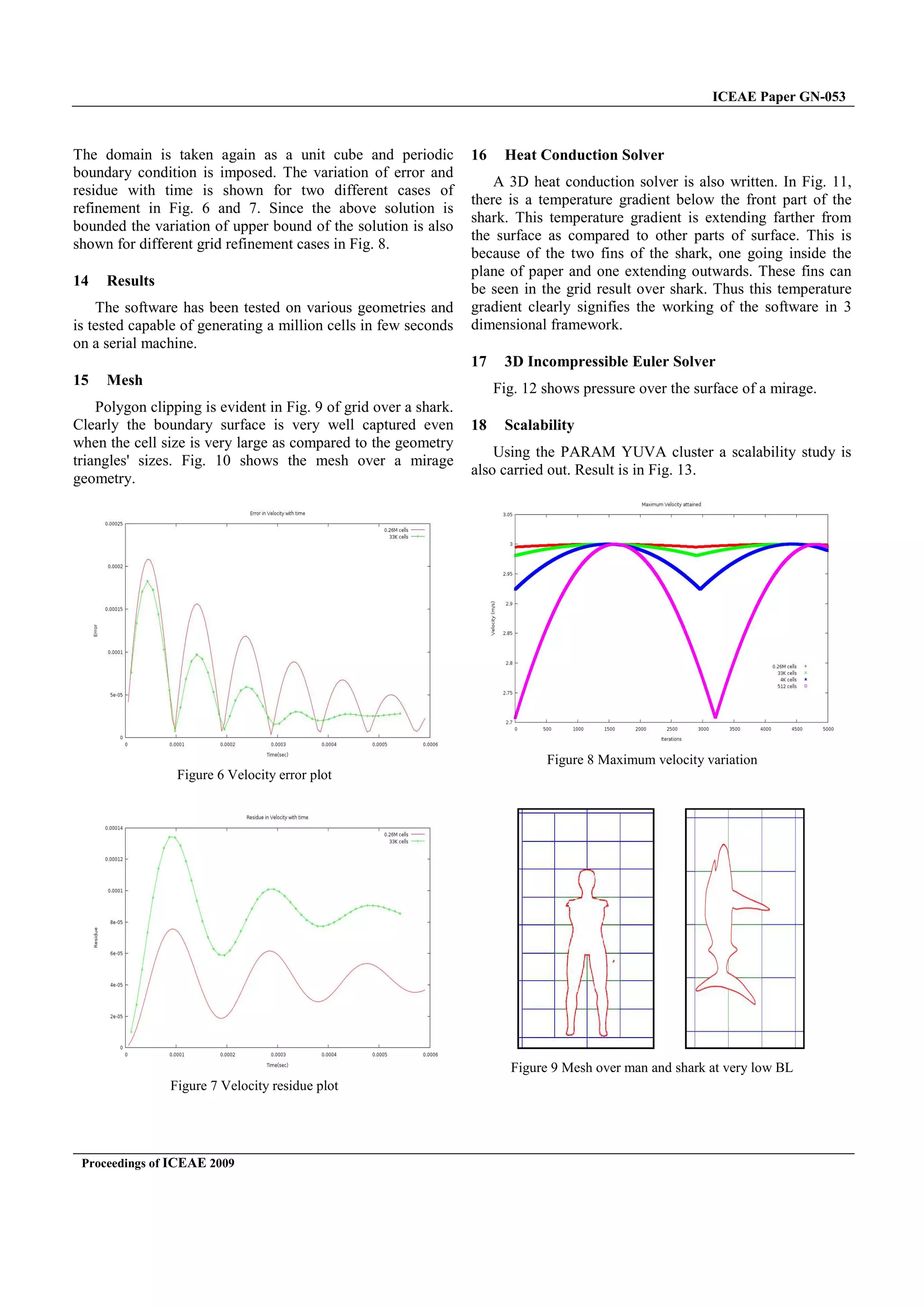
can be well captured. In Fig. 2, black region is the internal of
the geometry and the gray cells are candidates for being the
cut cells. Hence the cell to the right is divided because of the
constraint as shown by the dotted lines [7].
6 Inout function
To automatically generate cells and decide which cell
lies in which domain, a function which can tell whether a
point is inside or outside the geometry is required. The
'inout' function is a generalization of this requirement; it
determines the zone in which a point lies. The zones are
referred to space which is divided by various intersecting or
non intersecting water tight boundaries.
The function takes a point coordinate as input and then
fires a ray towards the positive x infinity. While doing so the
intersections with the various boundaries present in the space
is counted. If for a boundary, the ray crosses the boundary
odd number of times then the point lies inside that boundary
and if the ray crosses even number of times then the point
lies outside the boundary.
7 Grid geometry interactions
This is the most crucial part for any automatic meshing
algorithm where the level of accuracy of capturing the
geometry surface in the cut cells is decided. Since this level
directly dictates the fidelity of the solution, the present
algorithm achieves maximum possible accuracy in capturing
geometry surface inside the grid cells.
Each cell when created is populated with a list of
intersecting triangles. Here a geometry triangle may or may
not be associated with more than one grid cell depending
completely upon how many cells it intersects. Whenever a
bigger cell is divided to create new child cells, the list of
triangles of the parent cell gets distributed among the
children. Further, cut info stored in the parent cell is
discarded and the new cut info is found for newly generated
child cells. This is an important feature to allow AMR in the
region close to boundaries. Fig. 3 shows how a boundary
cell is divided into two parts by the geometry.
In order to find the exact grid geometry interactions, each
of the triangles associated with all the cells are clipped by
the respective cell boundaries. This is done using the
Sutherland-Hodgman polygon clipping algorithm. During
this process all triangles are clipped by all the cells they are
associated with. This gives a set of polygons in each
boundary cell which defines the cell cut info accurately to
the accuracy of the geometry input. Then the volume of each
cut cell is computed using divergence theorem on all the
faces of the cell and the clipped polygons present in that cell
[1][8].
8 Adaptive mesh refinement (AMR)
The basic grid which goes into the solver is generally
very coarse and meant to be subsequently refined as the
gradients develop across the coarse cells. The present
algorithm is capable of refining any particular cell or region
at any given time. This enables the solver algorithm to check
for high gradient cells in the computational domain and send
them for refinement after the solver iteration is complete.
Further, since the grid geometry interaction is dynamically
found as soon as a cell is generated there remains no
restriction on refining the grid at any point of time.
9 Parallelization
To run very complex solver algorithm on a large number
of cells parallelization is the only suitable method. For this
the mesh is divided into various zones where each of the
zones is solved by a single processor. The division of whole
mesh into zones is done using Hilbert-Peano space filling
curves which ensures minimum zone boundaries [9]. This is
required to minimise the intercommunication between
different processors.
In the zone division algorithm, each of the cells is given
a Hilbert value which arranges all the grid cells in a linear
manner. This Hilbert value is given using an algorithm given
by Hamilton [10]. Then depending on the total load of
computing cell cuts, the domain is partitioned such that each
processor gets equal load.
The parallelization has been tested on several nodes of
Synergy and PARAM YUVA clusters of Center for
Development of Advanced Computing (CDAC). Each of the
machines in the cluster has 64 GB RAM and 4 Xeon
Processors with each processor having 4 cores. On a single
node the code could generate 13 million leaf cells in 10
minutes.
Figure 3 Grid geometry interactions in a grid cell](https://image.slidesharecdn.com/research-paper-revisiting-projection-methods-over-automatic-oct-tree-meshes-201118092705/75/Revisiting-Projection-Methods-over-Automatic-Oct-tree-Meshes-3-2048.jpg)
![ICEAE Paper GN-053
Proceedings of ICEAE 2009
10 Incompressible Euler Solver
The solver in progress on the oct-tree mesh is for a
constant density and inviscid fluid. The work done is based
on the incompressible solver developed by Popinet in 2003
[7]. The velocity and pressure are dependent on three spatial
as well as temporal variables. Given as follows
ͱ{˲ ˳ ˴ ˮ{ ˯{˲ ˳ ˴ ˮ{
- ˰{˲ ˳ ˴ ˮ{ - ˱{˲ ˳ ˴ ˮ{˫
˜ ˜{˲ ˳ ˴ ˮ{
The Incompressible Euler equations used are
{ ͱ{ .˯{ ͱ{ . ˰{ ͱ{ . ˱{ ͱ{ . J
ͱ Ŵ
Apart from the standard inlet and outlet boundary
conditions the wall boundary is implemented with no
orthogonal flow component at the wall.
ͱ{˲ ˳ ˴ ˮ{ ; Ŵ ƒ– –Š‡ ™ƒŽŽ
where n is outward normal unit vector.
Projection method with fractional-step is used to solve
the above equations. In this method velocity U is known at
time t and pressure P at (t – ∆t/2). These values are stored at
the cell center.
As a first step in projection method U'' is computed using
the advection term.
ͱ ͱ
.V È$
,
In the above equation A is the advection term given by
[(U. )U].
In next step this U'' distribution is given to the projection
operator which gives the new velocity at (t+∆t). It also
updates the pressure field to the new pressure distribution at
(t+∆t/2).
11 Advection Term
The advection term is solved by applying divergence
theorem in each cell.
Vˮ- ˮÈŶ
ˤˢ
˕˥ˬˬ
{{ͱ {ͱ{ˮ- ˮÈŶ
ˤˢ
˕˥ˬˬ
{{ͱ {ͱ{ˮ- ˮÈŶ
ˤˢ
˕˥ˬˬ
ͱˮ- ˮÈŶ
˘II˥J
{ͱˮ- ˮÈŶ
;{ˤV
Rewriting the above equation for a cell in an oct-tree
mesh
Vˮ- ˮÈŶ
ŵ
ˢI˥ˬˬ
Ӝ ͱ˦II˥
ˮ- ˮÈŶ
ͱ˦II˥ ;
ˮ- ˮÈŶ
ӝ ˓˦II˥
˘II˥J
where Uface is the extrapolated velocity at the respective
face of the cell. Vcell is the volume of the cell and Aface is area
of the face in consideration. n is the outward normal unit
vector to the face.
The velocities are known at the center of the cell but to
calculate the advection term we need to extrapolate the
velocities at the faces. This extrapolation is performed using
Taylor series approximation. Hence the velocity at the face
can be calculated as follows
ͱˤˮ- ˮÈŶ ͱˮ
-
ˤ
Ŷ
ͱˮ
ˤ
-
ˮ
Ŷ
ͱˮ
ˮ
- ˛{ ˤŶ
ˮŶ
{
where d is the direction perpendicular to the plane of the
face, ∆d is the distance of the face from cell center. Now the
time derivative of velocity in the above equation can be
replaced by spatial derivatives using the Euler equations thus
giving
ͱ˲ˮ- ˮÈŶ ͱˮ
- @
˲
Ŷ
. ˯
ˮ
Ŷ
D
ͱˮ
˲
. ˰
ˮ
Ŷ
ͱˮ
˳
. ˱
ˮ
Ŷ
ͱˮ
˴
.
ˮ
Ŷ
˜ˮ
ͱ˳ˮ- ˮÈŶ ͱˮ
- @
˳
Ŷ
. ˰
ˮ
Ŷ
D
ͱˮ
˳
. ˯
ˮ
Ŷ
ͱˮ
˲
. ˱
ˮ
Ŷ
ͱˮ
˴
.
ˮ
Ŷ
˜ˮ
ͱ˴ˮ- ˮÈŶ ͱˮ
- @
˴
Ŷ
. ˱
ˮ
Ŷ
D
ͱˮ
˴
. ˯
ˮ
Ŷ
ͱˮ
˲
. ˰
ˮ
Ŷ
ͱˮ
˳
.
ˮ
Ŷ
˜ˮ
where Ux, Uy and Uz are velocities at the faces along x, y
and z directions respectively. Once the velocity at the face is
known from both sides of the cell simple upwinding is used
to decide the final velocity at the center of the face. But to
calculate the advection term we need normal velocity
component at the faces of a cell. Also for this method to
satisfy conservation equation the normal velocity should be
divergence free. Therefore to make the normal velocity
divergence free projection method is applied by solving the
following equation
˜ ˡ È$
where P is pressure at cell center, Ut+∆t/2
is velocity at the
face center. The resulting pressure field is then used to
correct the normal velocity component. Therefore the
corrected normal velocity is given by
˯ˤˮ- ˮÈŶ ˯ˤȊ . { ˜{ˤ
While correcting the normal velocities at the face center,
pressure gradient is also calculated at the cell center using
the gradient values at the faces of the cell. Calculation of
advection term also requires that the velocity is known at the
face center along with the normal component. It is done
using the same Taylor series approximation as mentioned
above. But this time the velocities for approximation are](https://image.slidesharecdn.com/research-paper-revisiting-projection-methods-over-automatic-oct-tree-meshes-201118092705/75/Revisiting-Projection-Methods-over-Automatic-Oct-tree-Meshes-4-2048.jpg)
![Bharat Raj Agrawal, Saurabh Pandey
Proceedings of ICEAE 2009
now taken as the average of the normal corrected velocities
at the faces of the cell as opposed to the cell centered
velocity. The final velocity is then calculated using the
equation
ͱˤˮ- ˮÈŶ ˡˤ
Ȋ
. ˜
Here Ud' is face centerd velocity calculated by applying
the Taylor series approximation and upwinding at the face.
P is the interpolated value of gradient at the face. The
linear interpolation is performed between the cells sharing
the face.
12 Projection Method
The projection method due to Chorin [11] is used to
update the velocity. According to this method intermediate
velocity is calculated by solving the momentum equation
ignoring the pressure variation. Then this intermediate
velocity is used to compute pressure field such that the
corrected velocity is divergence free. The projection method
utilizes the Helmholtz-Hodge decomposition of a vector
field U', which can be written as follows
ͱȊ
ͱˮ- ˮÈŶ
- ˜ (1)
where
ͱ È$
Ŵ (2)
and the boundary condition is
ͱ ; Ŵ
In general, the Helmholtz-Hodge decomposition of a
vector field describes it in two components, one a divergence
free vector field and the other is the gradient of a scalar field.
Taking divergence of (1) and using the divergence free
result of (2) will lead to the Poisson equation
Ŷ
˜ ͱȊ
Hence the final divergence free velocity is given by
ͱˮ- ˮÈŶ
ͱȊ
. ˜
13 Numerical Validation
The first set of numerical validation is performed on the
Poisson Solver. A unit cubical domain is taken with origin
situated at the center of the cube. The cells in the cubical
domain are initialized with the following divergence
ͱ{˲ ˳ ˴{ . ${˫$
- ˬ$
- ˭${ •‹{ ˫˲{ •‹{ ˬ˳{ •‹{ ˭˴{
with k = l = m = 1. The exact solution of the Poisson
Equation with the above divergence as the source term is
given by
˜{˲ ˳ ˴{ •‹{ ˫˲{ •‹{ ˬ˳{ •‹{ ˭˴{ - ˕ (3)
where C is a constant. The domain is initialized with a
constant zero pressure throughout the domain. The above
problem is simulated with variable number of cells in the
domain. The error in pressure is measured with respect to the
pressure given by (3) and residue is the change in pressure
compared to the last iteration. The results are shown in Fig.
4 and 5.
The validation of Euler Solver is performed by following
the work of Minion [12] and Almgren et al. [13] where the
whole domain is initialized with the following velocity
˯{˲ ˳{ ŵ . Ŷ …‘•{Ŷ ˲{ •‹{Ŷ ˳{
˰{˲ ˳{ ŵ - Ŷ •‹{Ŷ ˲{ …‘•{Ŷ ˳{
The exact solution of the Euler Equation for these initial
conditions is given by
˯{˲ ˳ ˮ{ ŵ . Ŷ …‘• Ŷ {˲ . ˮ{ •‹ Ŷ {˳ . ˮ{
˰{˲ ˳ ˮ{ ŵ - Ŷ •‹ Ŷ {˲ . ˮ{ …‘• Ŷ {˳ . ˮ{
˜{˲ ˳ ˮ{ .Ŷ …‘• Ÿ {˲ . ˮ{ . …‘• Ÿ {˳ . ˮ{
Figure 5 Error plot for Poisson solver
Figure 4 Residue plot for Poisson solver](https://image.slidesharecdn.com/research-paper-revisiting-projection-methods-over-automatic-oct-tree-meshes-201118092705/75/Revisiting-Projection-Methods-over-Automatic-Oct-tree-Meshes-5-2048.jpg)
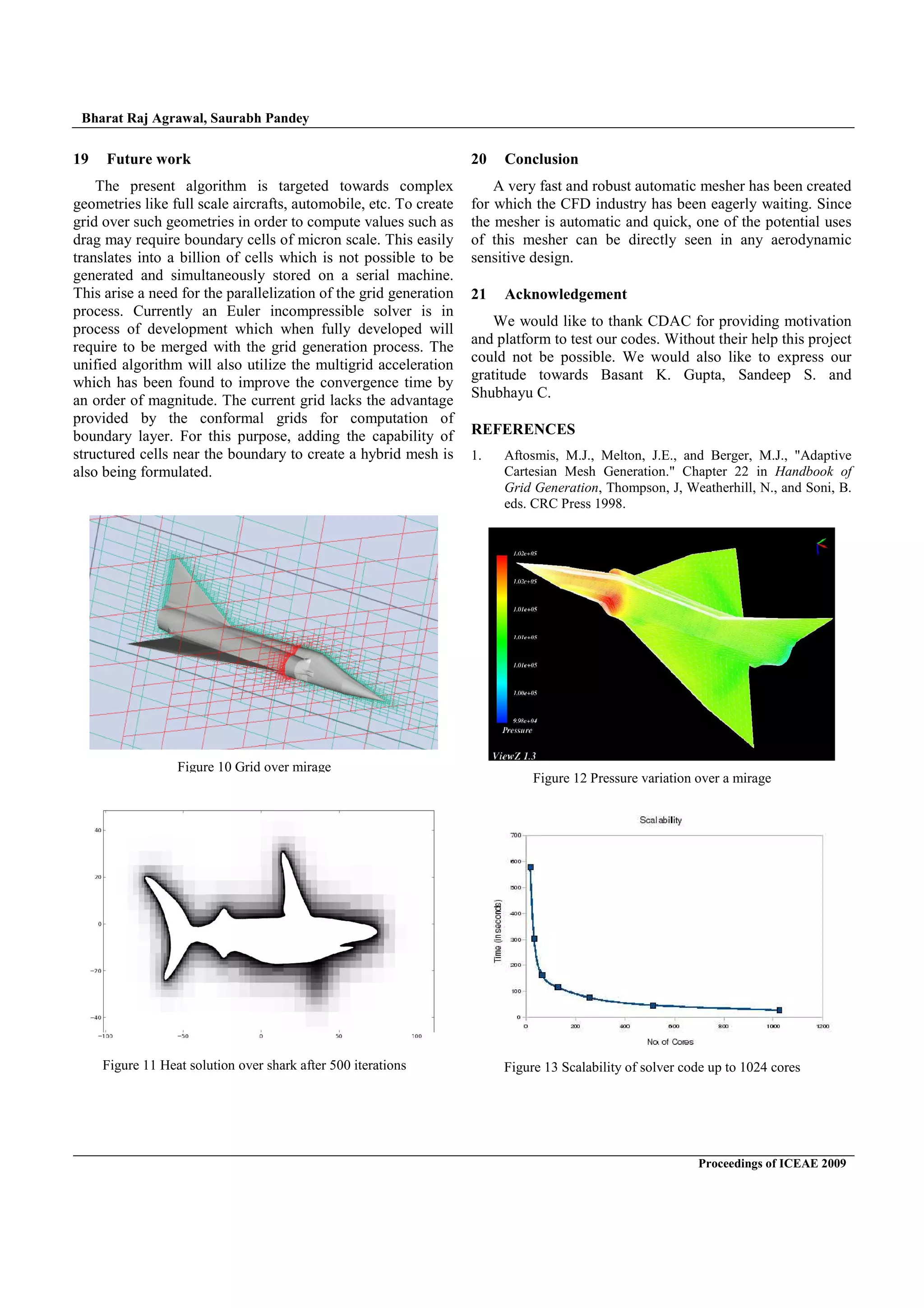

The document discusses an automatic oct-tree based cartesian mesh generation software designed to optimize grid creation for computational fluid dynamics (CFD), particularly over complex geometries. It details the algorithm's robust features, including the ability to create a large number of cells rapidly and accurately capture geometrical complexities, along with an incompressible Euler solver implemented on these meshes. The proposed method demonstrates significant potential to enhance simulations in CFD applications by reducing human intervention in grid generation while maintaining high accuracy in flow representation.