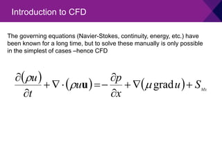
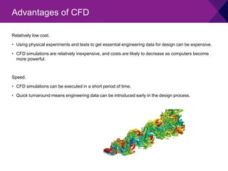
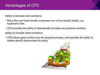
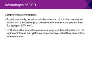
Dr Patrick Geoghegan
Book: H. Versteeg and W. Malalasekera An Introduction to
Computational Fluid Dynamics: The Finite Volume Method Chapter 2
FEA/CFD for
Biomedical
Engineering
Week 8: CFD –
Continuity
BIOFLUID SUMMARY
1st Year revision
• Hydrostatic Pressure
• Conservation of mass
• Bernoulli equation
BIOFLUID SUMMARY
𝑝𝑝1 − 𝑝𝑝2 = 𝜌𝜌𝜌𝜌𝜌
̇
𝑚𝑚 = 𝑐𝑐𝑐𝑐𝑐𝑐𝑐𝑐𝑐𝑐𝑐𝑐𝑐𝑐𝑐𝑐 = 𝜌𝜌1𝐴𝐴1𝑢𝑢1 = 𝜌𝜌2𝐴𝐴2𝑢𝑢2
𝑝𝑝1 +
1
2
𝜌𝜌𝑢𝑢1
2
+ 𝜌𝜌𝑔𝑔ℎ1 = 𝑝𝑝2 +
1
2
𝜌𝜌𝑢𝑢2
2
+ 𝜌𝜌𝑔𝑔ℎ2
Viscosity and Blood Rheology
• Shear stress
• Kinematic Viscosity
BIOFLUID SUMMARY
𝜏𝜏 = 𝜇𝜇
𝑑𝑑𝑑𝑑
𝑑𝑑𝑑𝑑
𝜇𝜇 = 𝜈𝜈𝜈𝜈
• Pressure Gradient in a pipe
• Pressure loss fully developed flow
• Poiseuille Parabolic profile
• Average Velocity
BIOFLUID SUMMARY
Δ𝑝𝑝 =
8𝜇𝜇𝜇𝜇𝜇𝜇
𝜋𝜋𝑅𝑅4
𝑢𝑢 = 2�
𝑈𝑈 1 −
𝑟𝑟2
𝑅𝑅2
�
𝑈𝑈 =
𝑄𝑄
𝜋𝜋𝑅𝑅2
• Boundary Layer
• Boundary layer thickness (u=0.99U)
• Pipe entrance length
• Reynolds Number
• For smooth pipes of circular cross section:
• Laminar flow: Re < ~2300-2500
• Transitional flow: ~2300-2500 < Re < 4000
• Turbulent flow: Re > 4000
BIOFLUID SUMMARY
𝑋𝑋 = 0.06𝑑𝑑 𝑅𝑅𝑅𝑅
𝑅𝑅𝑅𝑅 =
𝜌𝜌𝜌𝜌𝜌𝜌
𝜇𝜇
=
𝑈𝑈𝑈𝑈
𝜈𝜈
𝑅𝑅𝑅𝑅 =
𝑈𝑈𝑈𝑈
𝜈𝜈
Laminar Flow
• Path line each particles are parallel
• Low velocity
• Viscosity plays a significant part in laminar
• Velocity profile shown as parabolic curve
Turbulent Flow
• Particles are irregular path line
• High velocity
• Inertia plays a significant part in turbulent
• Velocity profile shown as logarithm curve
BIOFLUID SUMMARY
• Womersley Number
• Angular Frequency
• Flow rate in a venturi
• Wall Shear Stress
Equation Overview
𝛼𝛼 =
𝑑𝑑
2
𝜔𝜔
𝜈𝜈
=
𝑑𝑑
2
𝜔𝜔𝜔𝜔
𝜇𝜇
𝜔𝜔 = 2𝜋𝜋𝜋𝜋 =
2𝜋𝜋
𝑇𝑇
𝑄𝑄 =
2∆𝑝𝑝
𝜌𝜌 ⁄
1 𝐴𝐴2
2
− ⁄
1 𝐴𝐴1
2
𝜏𝜏 = 𝜇𝜇 �
𝑑𝑑𝑑𝑑
𝑑𝑑𝑑𝑑 𝑧𝑧=0
0 0.2 0.4 0.6 0.8 1
200
400
600
800
1000
Re
t / τ
0 0.2 0.4 0.6 0.8 1
1.5
1.7
1.9
2.1
2.3
2.5
2.7
2.9
3.1
x 10
4
Pressure
(Pa)
0 0.2 0.4 0.6 0.8 1
1.5
1.7
1.9
2.1
2.3
2.5
2.7
2.9
3.1
x 10
4
Pressure
(Pa)
CFD Basics Part 1
Computational fluid dynamics (CFD) is the science of predicting fluid flow, heat transfer, mass transfer,
chemical reactions, and related phenomena by solving the mathematical equations which govern these
processes using a numerical process.
Introduction to CFD
The governing equations (Navier-Stokes, continuity, energy, etc.) have
been known for a long time, but to solve these manually is only possible
in the simplest of cases –hence CFD
Introduction to CFD
( ) ( ) ( ) Mx
S
u
x
p
u
t
u
+
∇
+
∂
∂
−
=
⋅
∇
+
∂
∂
grad
µ
ρ
ρ
u
Relatively low cost.
• Using physical experiments and tests to get essential engineering data for design can be expensive.
• CFD simulations are relatively inexpensive, and costs are likely to decrease as computers become
more powerful.
Speed.
• CFD simulations can be executed in a short period of time.
• Quick turnaround means engineering data can be introduced early in the design process.
Advantages of CFD
Ability to simulate real conditions.
• Many flow and heat transfer processes can not be (easily) tested, e.g.
hypersonic flow.
• CFD provides the ability to theoretically simulate any physical condition.
Ability to simulate ideal conditions.
• CFD allows great control over the physical process, and provides the ability to
isolate specific phenomena for study.
Advantages of CFD
Comprehensive information.
• Experiments only permit data to be extracted at a limited number of
locations in the system (e.g. pressure and temperature probes, heat
flux gauges, LDV, etc.).
• CFD allows the analyst to examine a large number of locations in the
region of interest, and yields a comprehensive set of flow parameters
for examination.
Advantages of CFD
Physical models.
• CFD solutions rely upon physical models of real world processes (e.g.
turbulence, compressibility, chemistry, multiphase flow, etc.).
• The CFD solutions can only be as accurate as the physical models on
which they are based.
Boundary conditions
• As with physical models, the accuracy of the CFD solution is only as
good as the initial/boundary conditions provided to the numerical model
Rubbish in = Rubbish Out!
Limitations of CFD

Part 1 Biofluids Summary and CFD basics Pt 1(1).pdf

  • 1.
    Dr Patrick Geoghegan Book:H. Versteeg and W. Malalasekera An Introduction to Computational Fluid Dynamics: The Finite Volume Method Chapter 2 FEA/CFD for Biomedical Engineering Week 8: CFD – Continuity
  • 2.
  • 3.
    1st Year revision •Hydrostatic Pressure • Conservation of mass • Bernoulli equation BIOFLUID SUMMARY 𝑝𝑝1 − 𝑝𝑝2 = 𝜌𝜌𝜌𝜌𝜌 ̇ 𝑚𝑚 = 𝑐𝑐𝑐𝑐𝑐𝑐𝑐𝑐𝑐𝑐𝑐𝑐𝑐𝑐𝑐𝑐 = 𝜌𝜌1𝐴𝐴1𝑢𝑢1 = 𝜌𝜌2𝐴𝐴2𝑢𝑢2 𝑝𝑝1 + 1 2 𝜌𝜌𝑢𝑢1 2 + 𝜌𝜌𝑔𝑔ℎ1 = 𝑝𝑝2 + 1 2 𝜌𝜌𝑢𝑢2 2 + 𝜌𝜌𝑔𝑔ℎ2
  • 4.
    Viscosity and BloodRheology • Shear stress • Kinematic Viscosity BIOFLUID SUMMARY 𝜏𝜏 = 𝜇𝜇 𝑑𝑑𝑑𝑑 𝑑𝑑𝑑𝑑 𝜇𝜇 = 𝜈𝜈𝜈𝜈
  • 5.
    • Pressure Gradientin a pipe • Pressure loss fully developed flow • Poiseuille Parabolic profile • Average Velocity BIOFLUID SUMMARY Δ𝑝𝑝 = 8𝜇𝜇𝜇𝜇𝜇𝜇 𝜋𝜋𝑅𝑅4 𝑢𝑢 = 2� 𝑈𝑈 1 − 𝑟𝑟2 𝑅𝑅2 � 𝑈𝑈 = 𝑄𝑄 𝜋𝜋𝑅𝑅2
  • 6.
    • Boundary Layer •Boundary layer thickness (u=0.99U) • Pipe entrance length • Reynolds Number • For smooth pipes of circular cross section: • Laminar flow: Re < ~2300-2500 • Transitional flow: ~2300-2500 < Re < 4000 • Turbulent flow: Re > 4000 BIOFLUID SUMMARY 𝑋𝑋 = 0.06𝑑𝑑 𝑅𝑅𝑅𝑅 𝑅𝑅𝑅𝑅 = 𝜌𝜌𝜌𝜌𝜌𝜌 𝜇𝜇 = 𝑈𝑈𝑈𝑈 𝜈𝜈 𝑅𝑅𝑅𝑅 = 𝑈𝑈𝑈𝑈 𝜈𝜈
  • 7.
    Laminar Flow • Pathline each particles are parallel • Low velocity • Viscosity plays a significant part in laminar • Velocity profile shown as parabolic curve Turbulent Flow • Particles are irregular path line • High velocity • Inertia plays a significant part in turbulent • Velocity profile shown as logarithm curve BIOFLUID SUMMARY
  • 8.
    • Womersley Number •Angular Frequency • Flow rate in a venturi • Wall Shear Stress Equation Overview 𝛼𝛼 = 𝑑𝑑 2 𝜔𝜔 𝜈𝜈 = 𝑑𝑑 2 𝜔𝜔𝜔𝜔 𝜇𝜇 𝜔𝜔 = 2𝜋𝜋𝜋𝜋 = 2𝜋𝜋 𝑇𝑇 𝑄𝑄 = 2∆𝑝𝑝 𝜌𝜌 ⁄ 1 𝐴𝐴2 2 − ⁄ 1 𝐴𝐴1 2 𝜏𝜏 = 𝜇𝜇 � 𝑑𝑑𝑑𝑑 𝑑𝑑𝑑𝑑 𝑧𝑧=0 0 0.2 0.4 0.6 0.8 1 200 400 600 800 1000 Re t / τ 0 0.2 0.4 0.6 0.8 1 1.5 1.7 1.9 2.1 2.3 2.5 2.7 2.9 3.1 x 10 4 Pressure (Pa) 0 0.2 0.4 0.6 0.8 1 1.5 1.7 1.9 2.1 2.3 2.5 2.7 2.9 3.1 x 10 4 Pressure (Pa)
  • 9.
  • 10.
    Computational fluid dynamics(CFD) is the science of predicting fluid flow, heat transfer, mass transfer, chemical reactions, and related phenomena by solving the mathematical equations which govern these processes using a numerical process. Introduction to CFD
  • 11.
    The governing equations(Navier-Stokes, continuity, energy, etc.) have been known for a long time, but to solve these manually is only possible in the simplest of cases –hence CFD Introduction to CFD ( ) ( ) ( ) Mx S u x p u t u + ∇ + ∂ ∂ − = ⋅ ∇ + ∂ ∂ grad µ ρ ρ u
  • 12.
    Relatively low cost. •Using physical experiments and tests to get essential engineering data for design can be expensive. • CFD simulations are relatively inexpensive, and costs are likely to decrease as computers become more powerful. Speed. • CFD simulations can be executed in a short period of time. • Quick turnaround means engineering data can be introduced early in the design process. Advantages of CFD
  • 13.
    Ability to simulatereal conditions. • Many flow and heat transfer processes can not be (easily) tested, e.g. hypersonic flow. • CFD provides the ability to theoretically simulate any physical condition. Ability to simulate ideal conditions. • CFD allows great control over the physical process, and provides the ability to isolate specific phenomena for study. Advantages of CFD
  • 14.
    Comprehensive information. • Experimentsonly permit data to be extracted at a limited number of locations in the system (e.g. pressure and temperature probes, heat flux gauges, LDV, etc.). • CFD allows the analyst to examine a large number of locations in the region of interest, and yields a comprehensive set of flow parameters for examination. Advantages of CFD
  • 15.
    Physical models. • CFDsolutions rely upon physical models of real world processes (e.g. turbulence, compressibility, chemistry, multiphase flow, etc.). • The CFD solutions can only be as accurate as the physical models on which they are based. Boundary conditions • As with physical models, the accuracy of the CFD solution is only as good as the initial/boundary conditions provided to the numerical model Rubbish in = Rubbish Out! Limitations of CFD