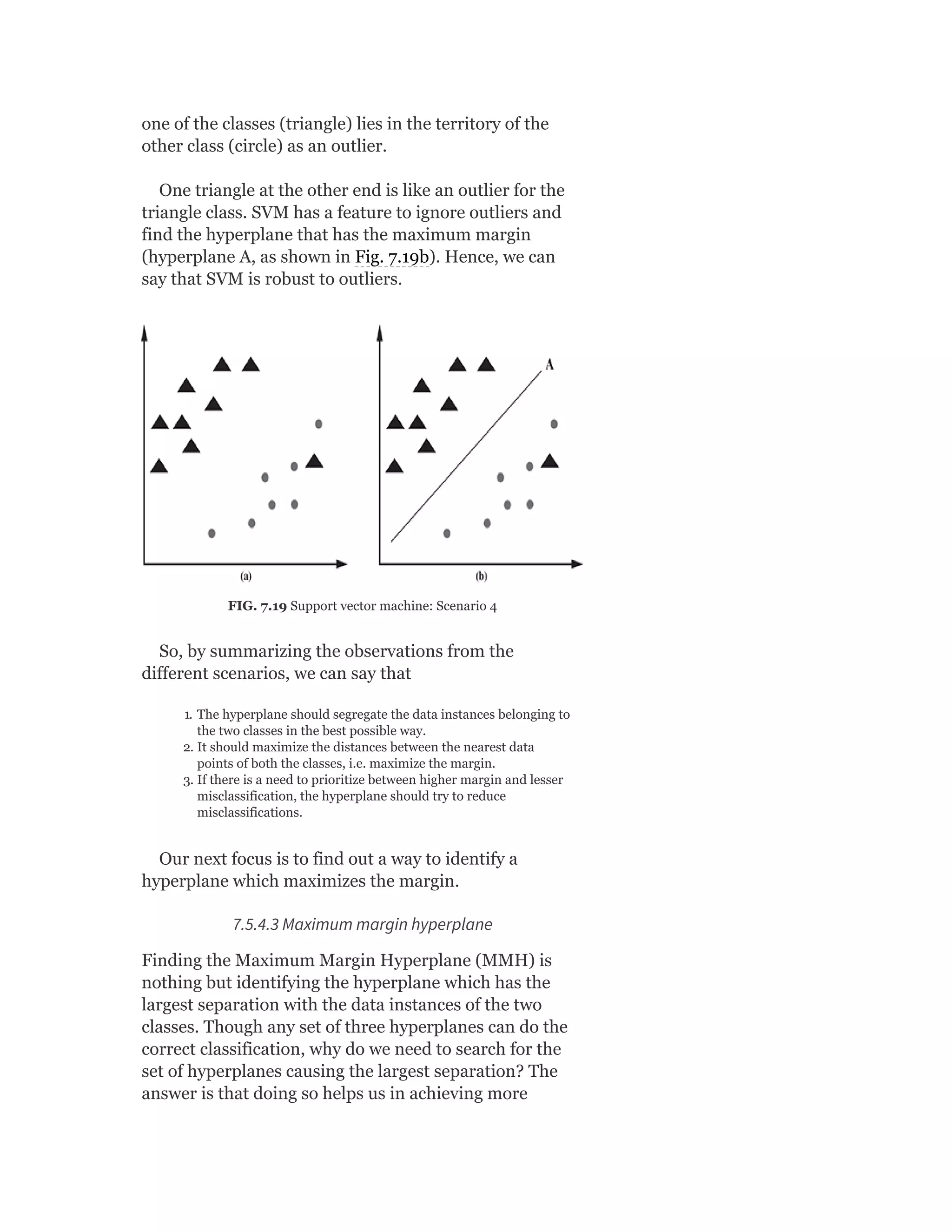
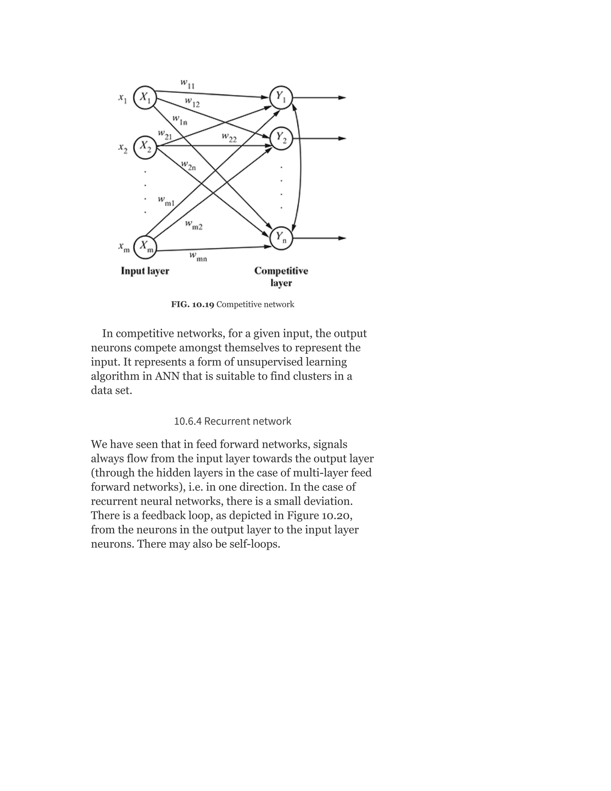
Pearson is the world's largest education company, operating in over 70 countries. They work closely with educators and thought leaders to develop high-quality educational products across higher education and K-12. Pearson believes that education opens opportunities and improves lives. Their goal is to provide superior learning experiences and outcomes through products developed with leading experts. Users are encouraged to provide feedback to help Pearson continue improving.


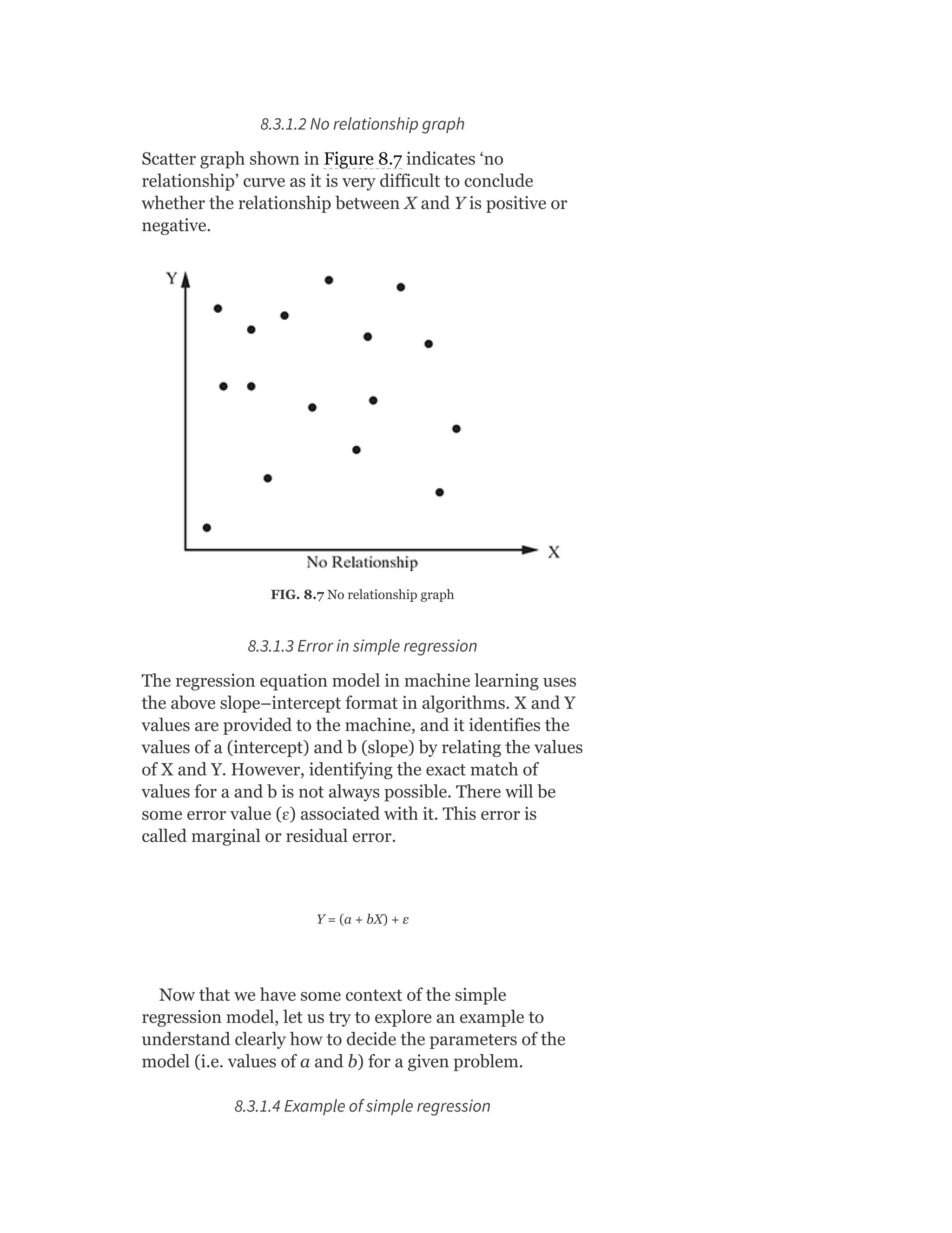
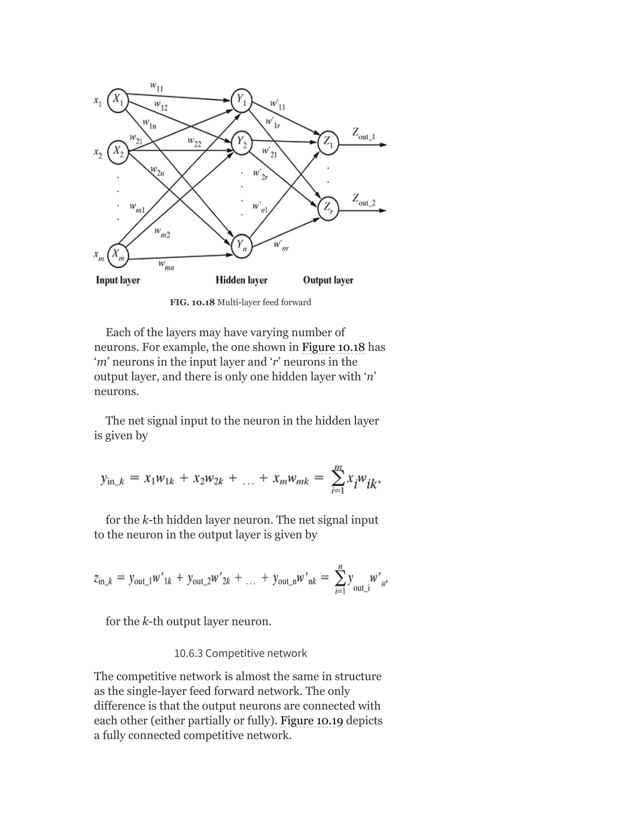
![Model Syllabus for Machine Learning
Credits: 5
Contacts per week: 3 lectures + 1 tutorial
MODULE I
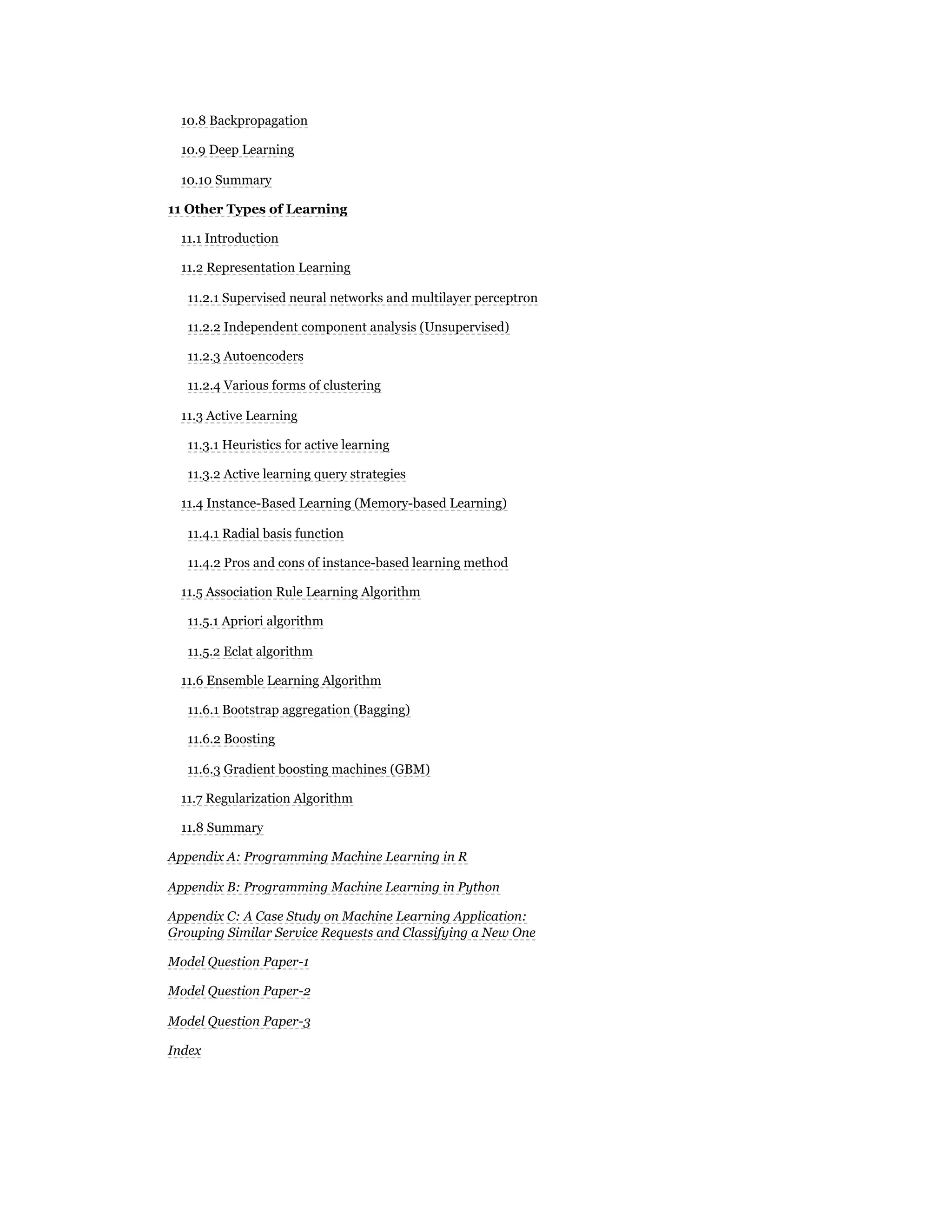
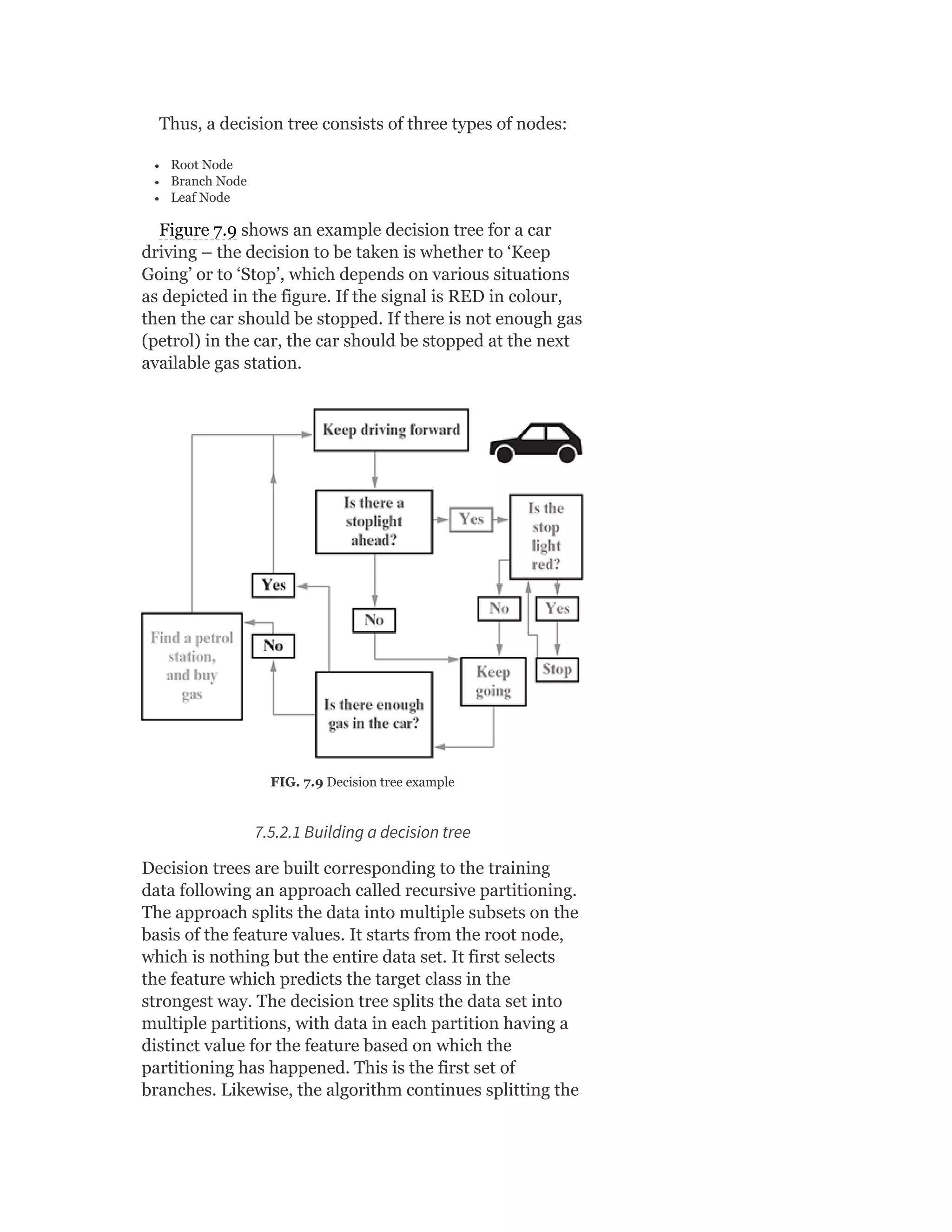
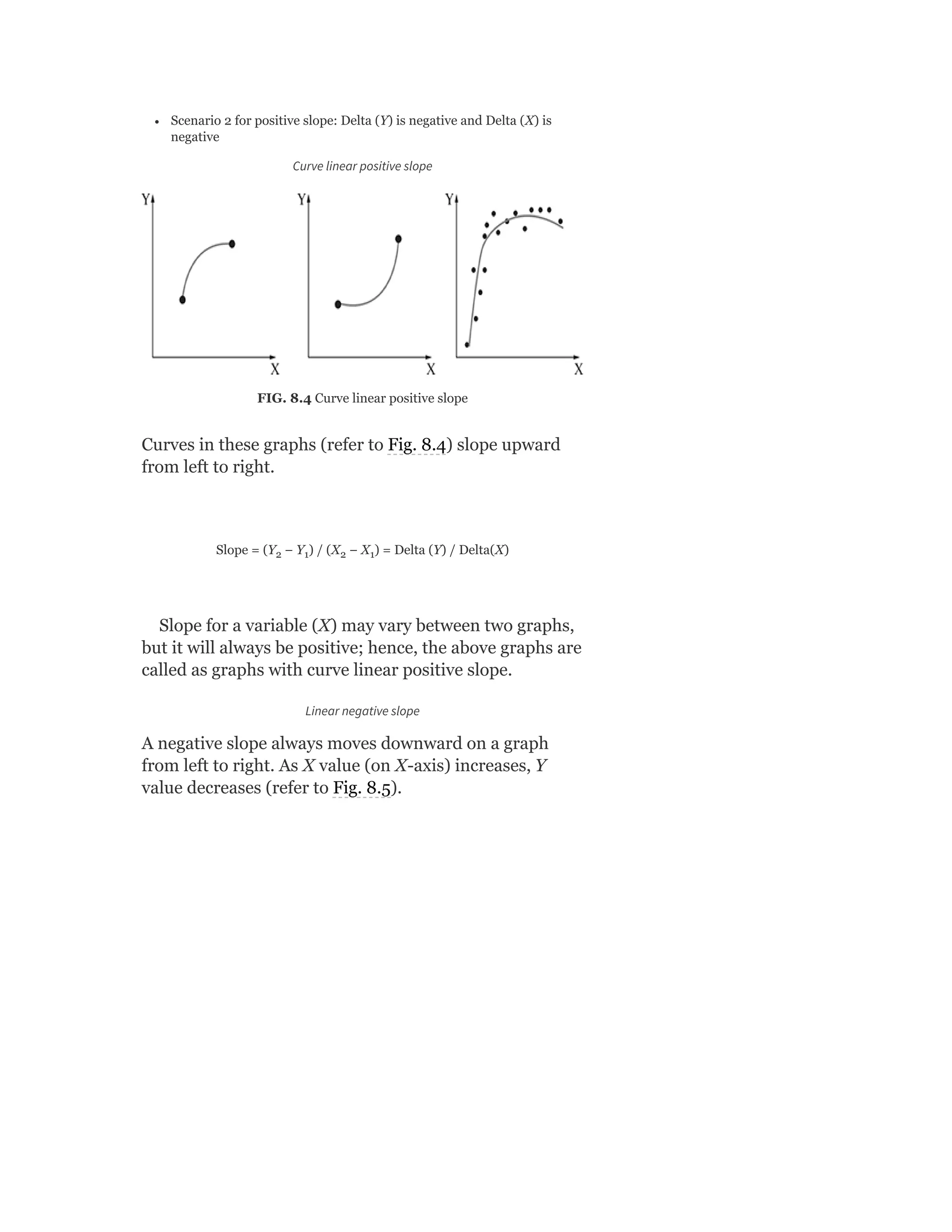
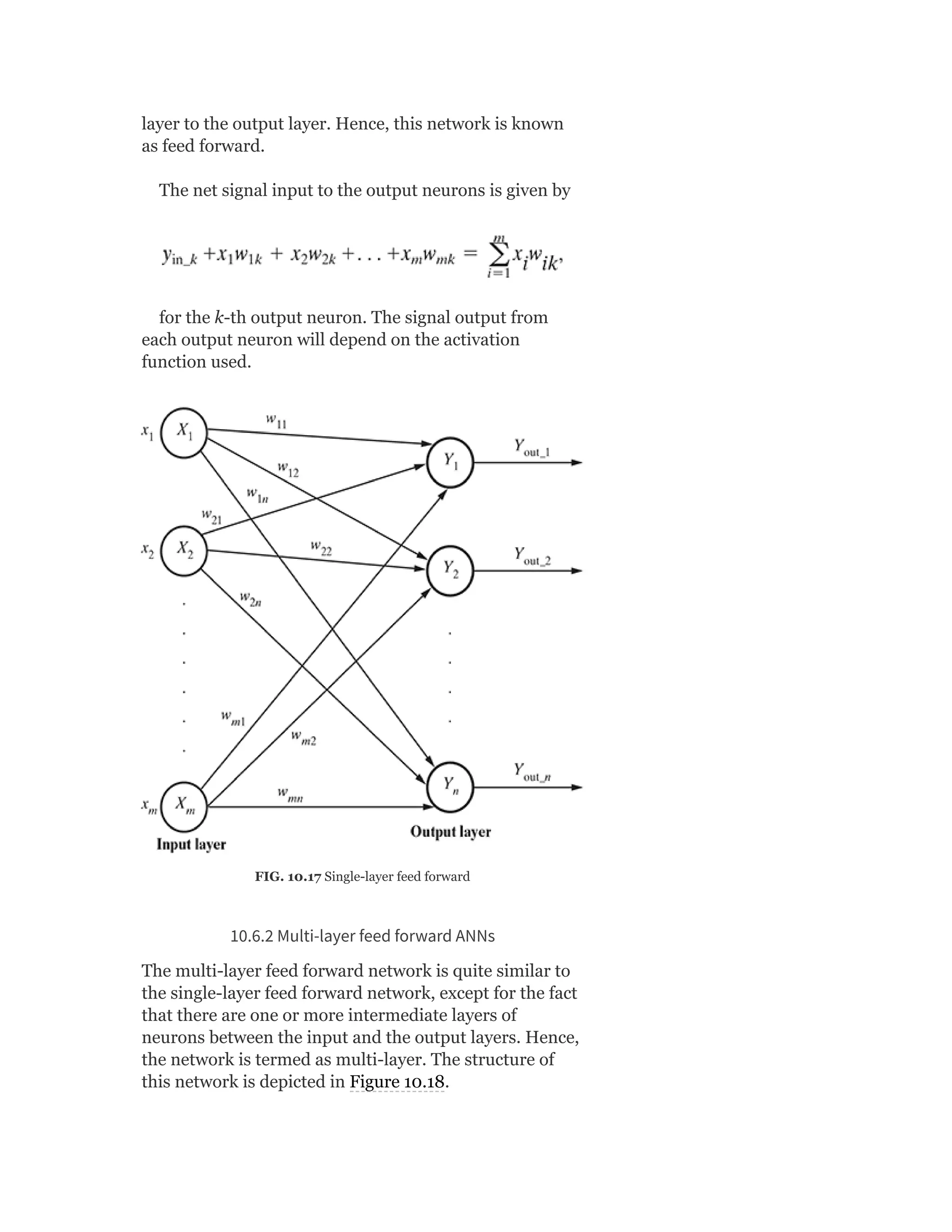
Introduction to Machine Learning: Human
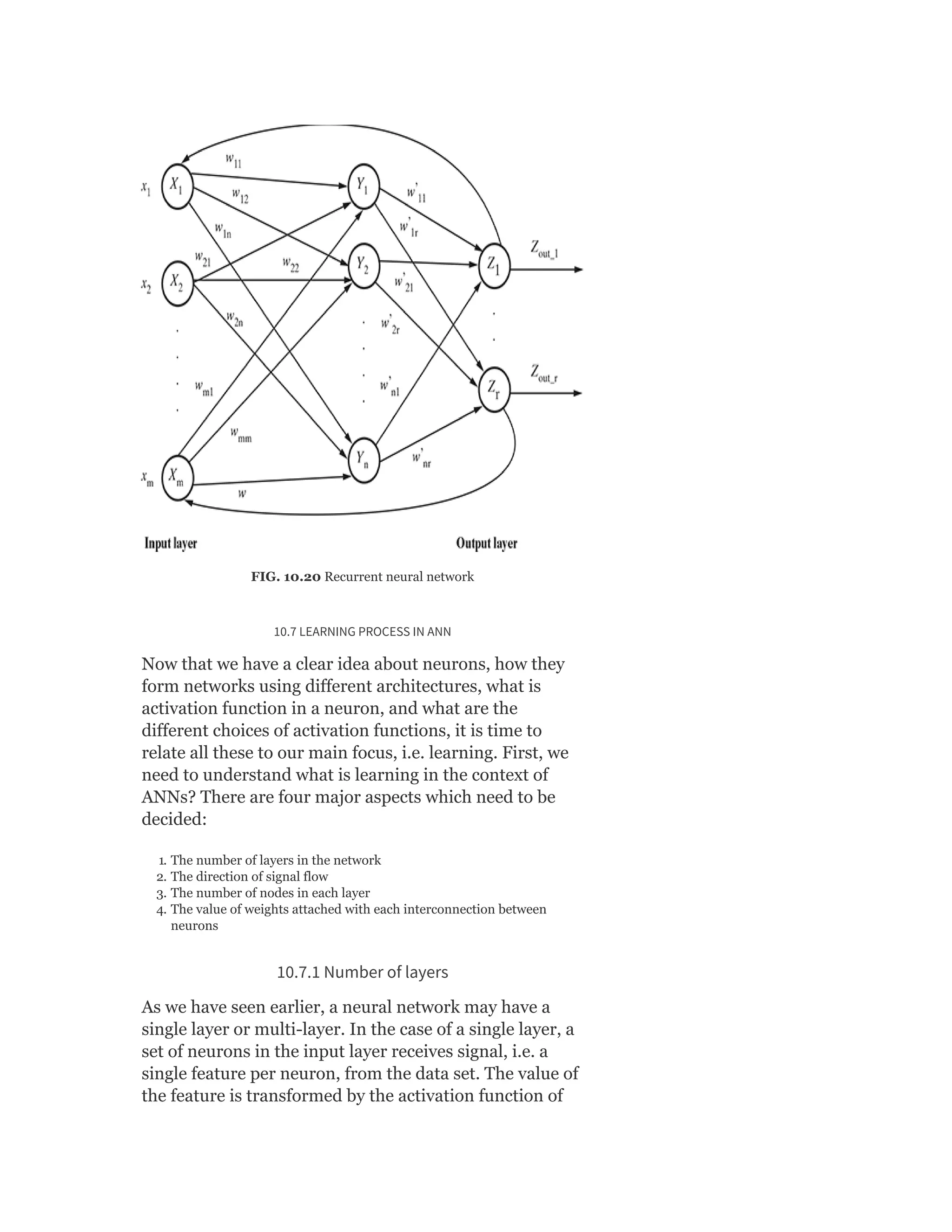
learning and it’s types; Machine learning and it’s types;
well-posed learning problem; applications of machine
learning; issues in machine learning
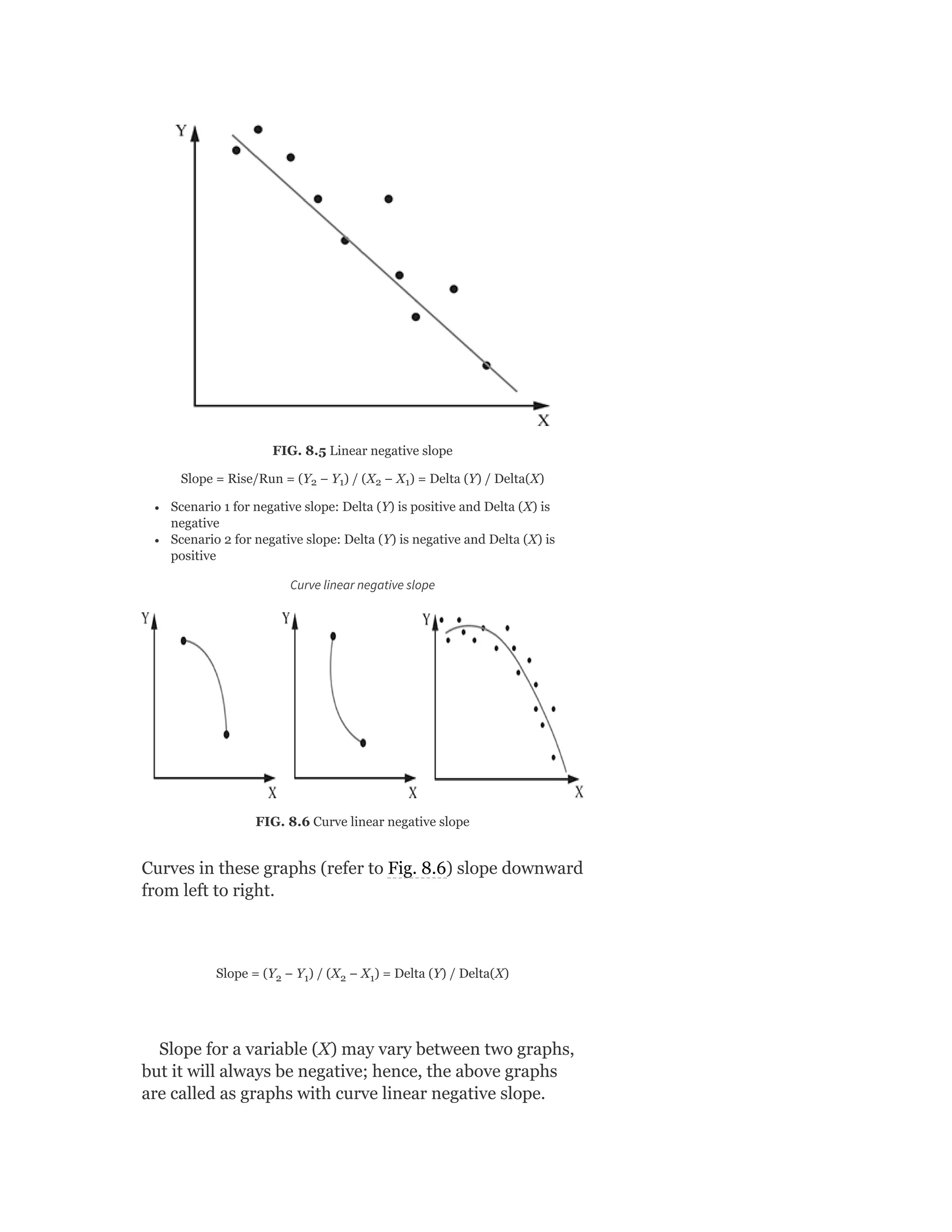
Preparing to model: Basic data types; exploring
numerical data; exploring categorical data; exploring
relationship between variables; data issues and
remediation; data pre-processing
Modelling and Evaluation: Selecting a model;
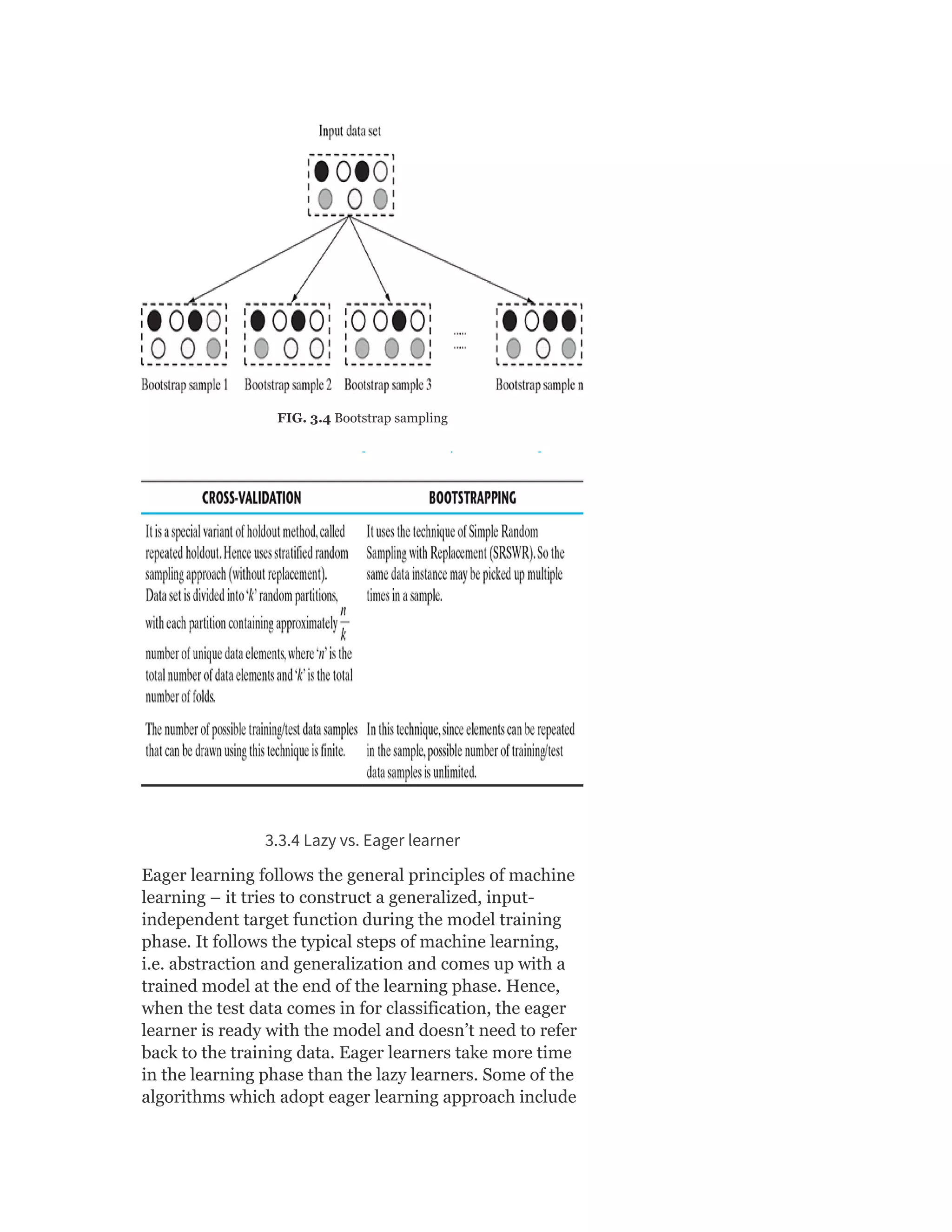
training model – holdout, k-fold cross-validation,
bootstrap sampling; model representation and
interpretability – under-fitting, over-fitting, bias-
variance tradeoff; model performance evaluation –
classification, regression, clustering; performance
improvement
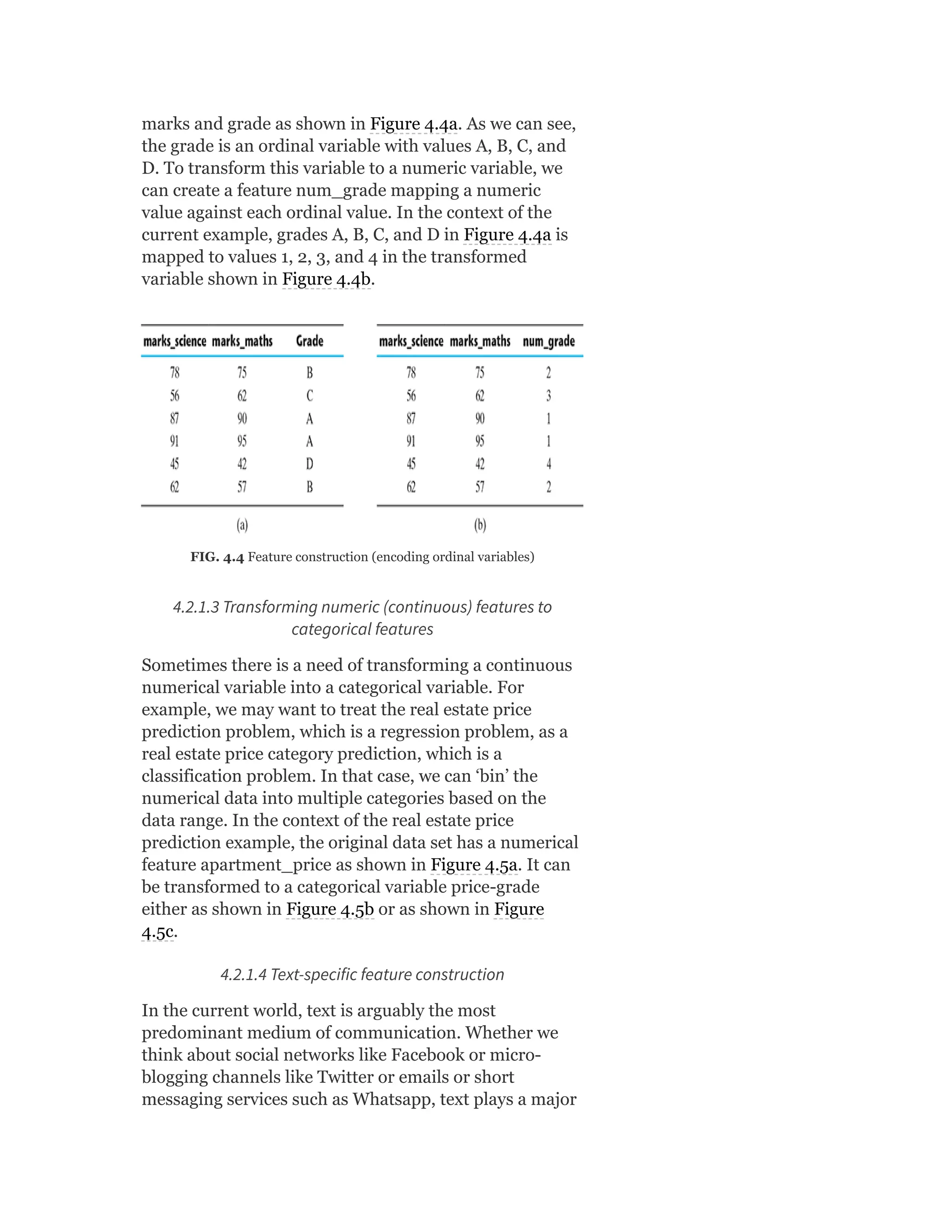
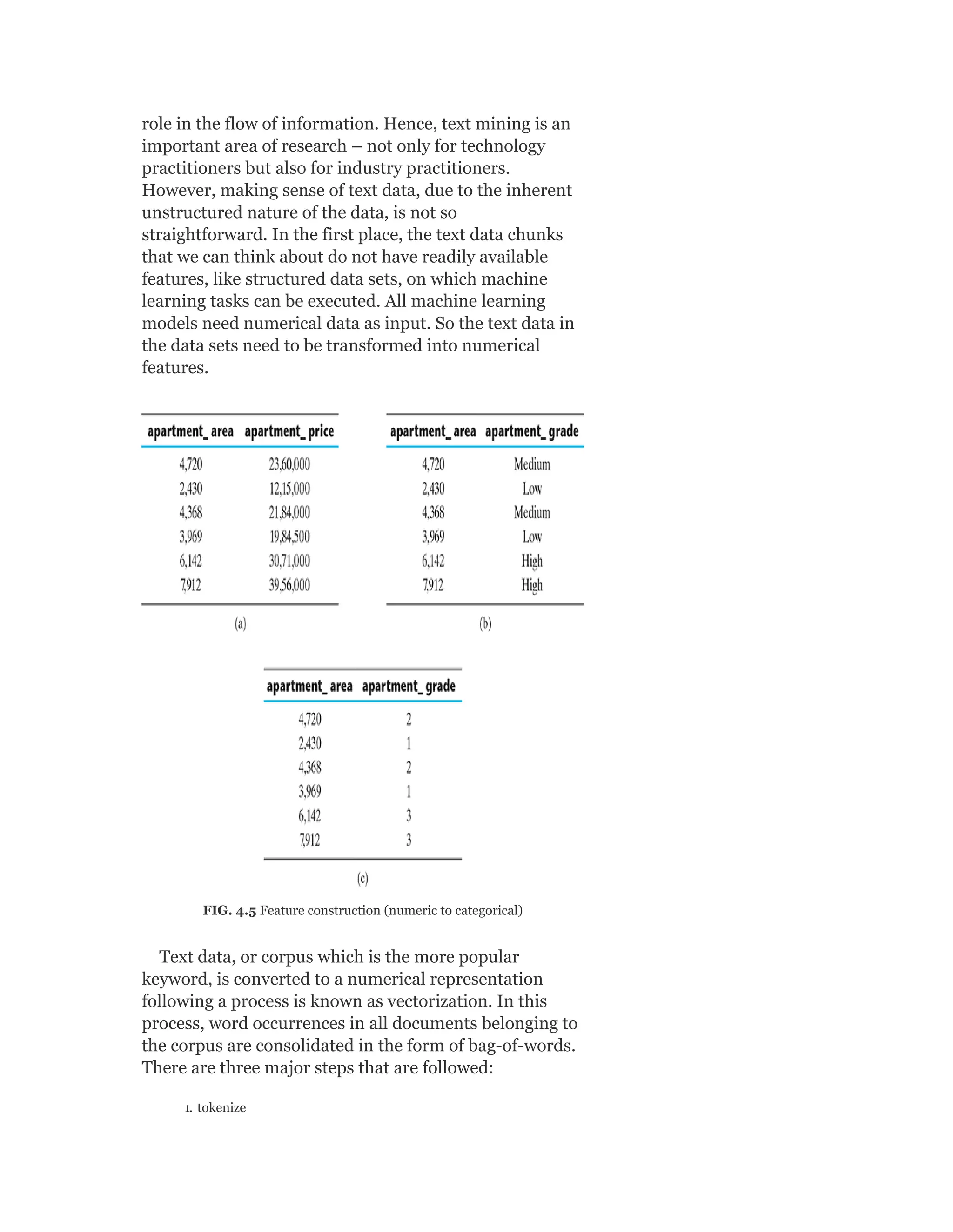
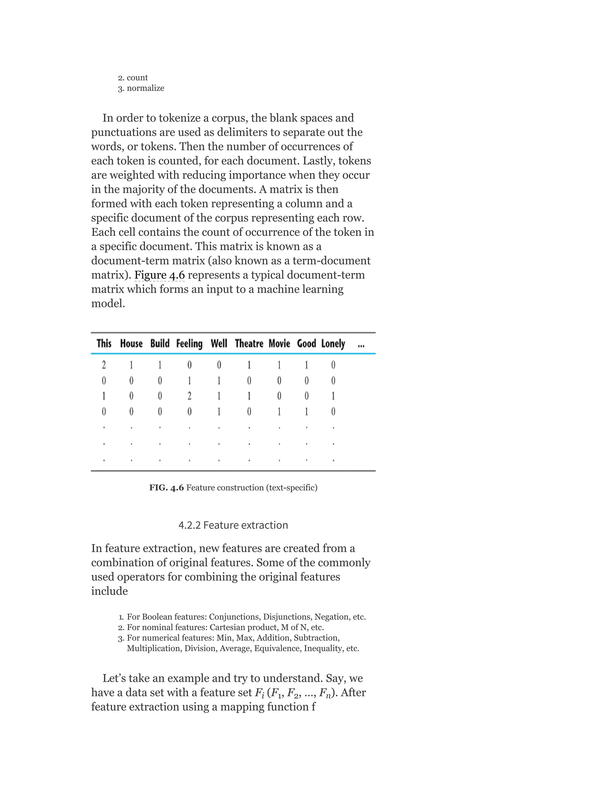
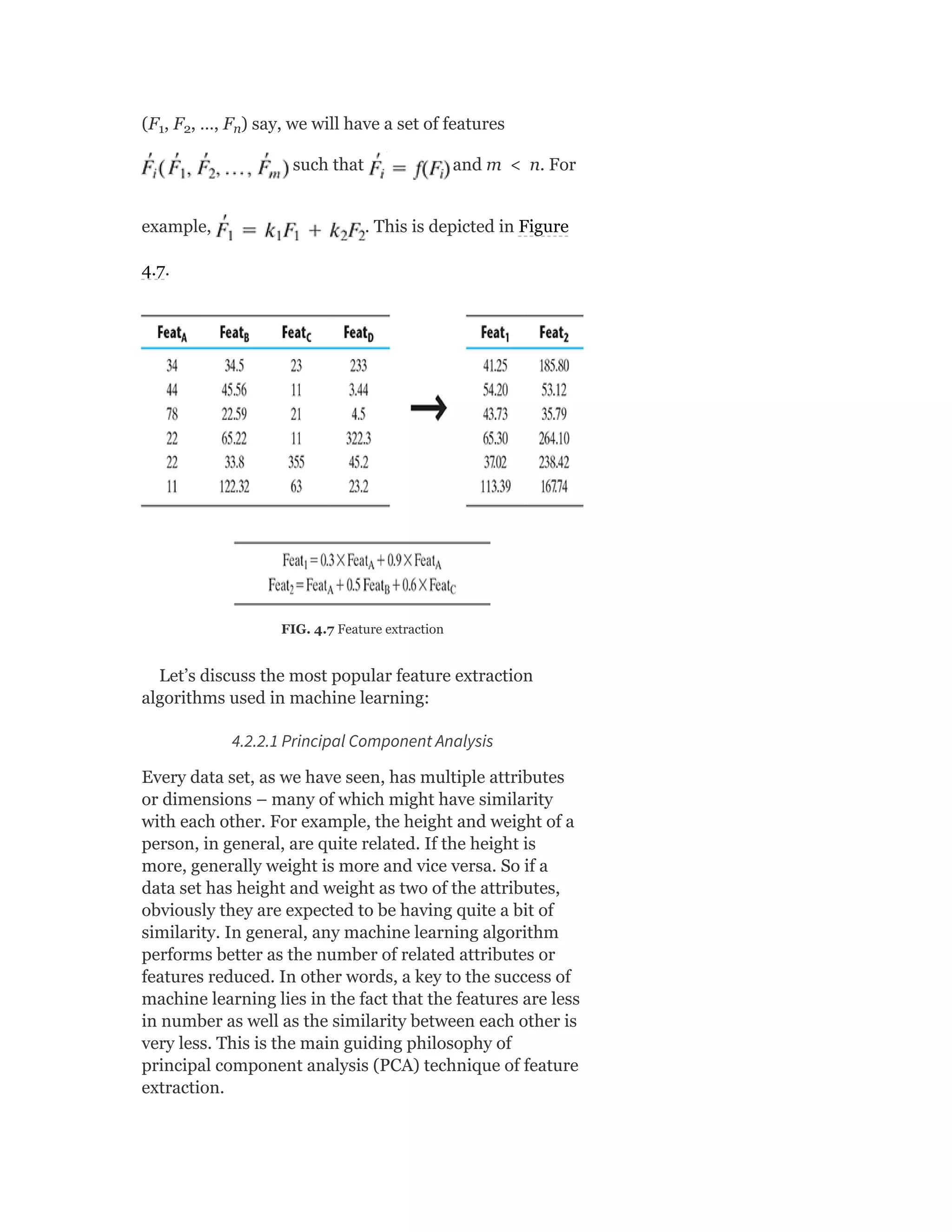
Feature engineering: Feature construction; feature
extraction; feature selection
[12 Lectures]
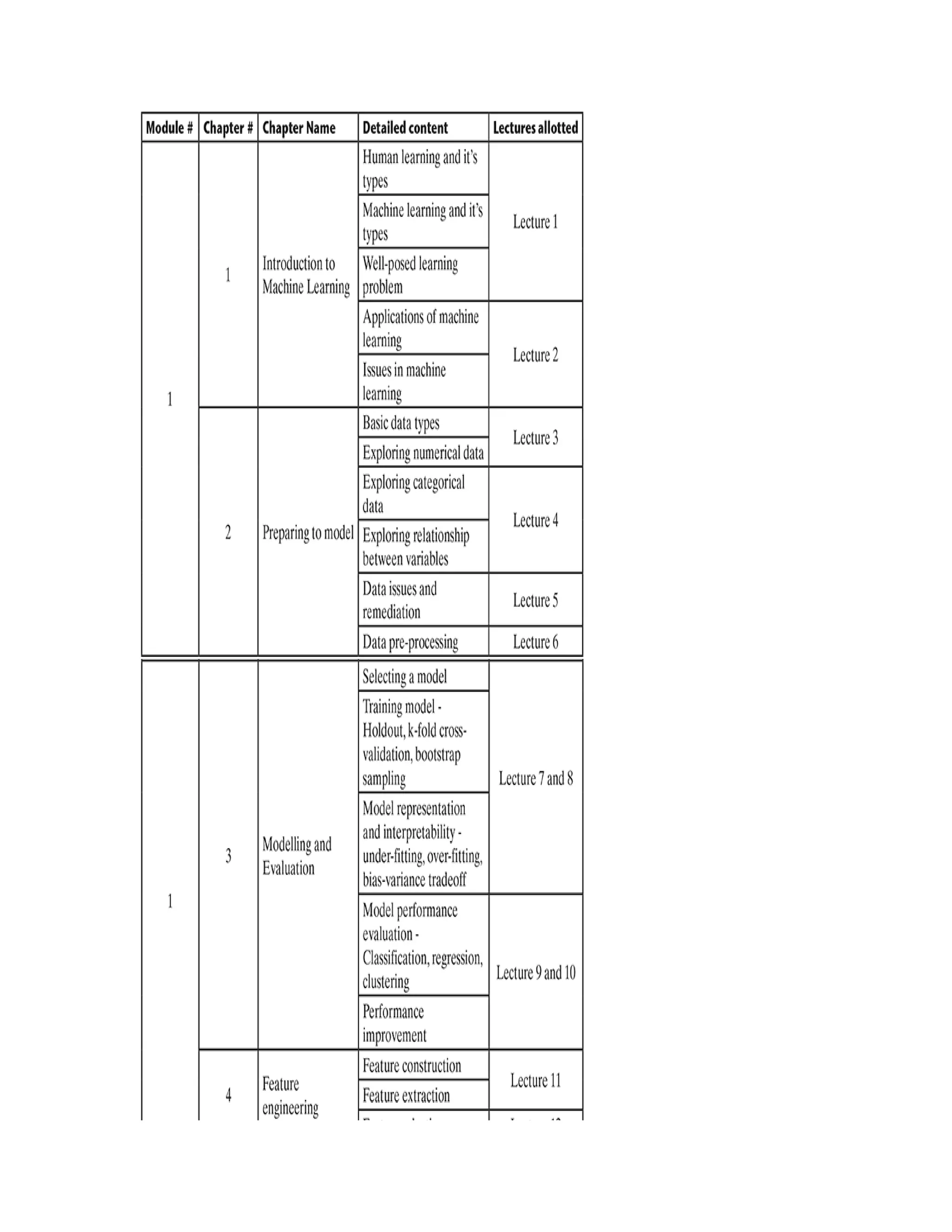
MODULE II
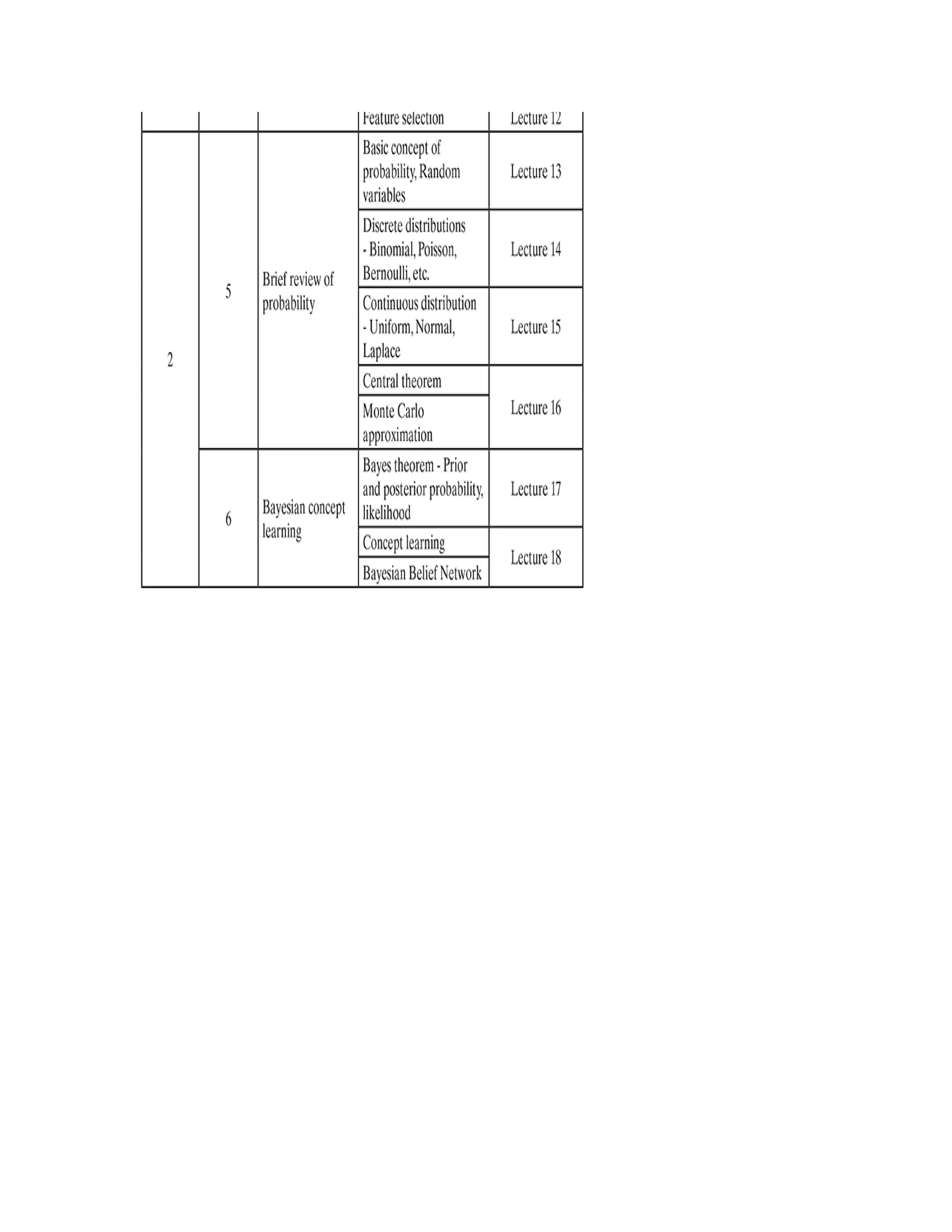
Brief review of probability: Basic concept of
probability, random variables; discrete distributions –
binomial, Poisson, Bernoulli, etc.; continuous
distribution – uniform, normal, Laplace; central
theorem; Monte Carlo approximation
Bayesian concept learning: Bayes theorem – prior
and posterior probability, likelihood; concept learning;](https://image.slidesharecdn.com/mlsaikatdutt-221115120700-3df1a1af/75/ML_saikat-dutt-pdf-23-2048.jpg)
![Bayesian Belief Network
[6 Lectures]
MODULE III
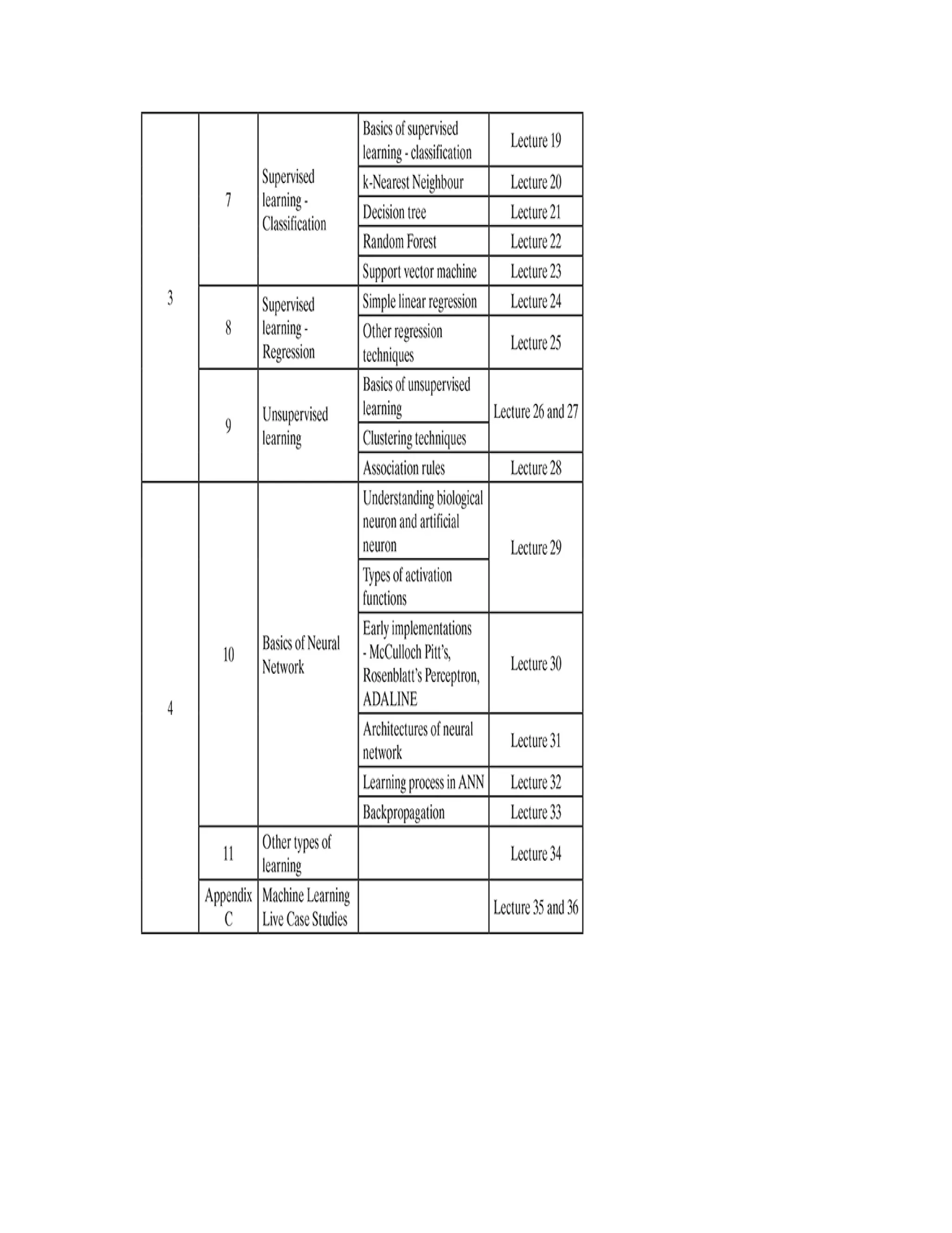
Supervised learning – Classification: Basics of
supervised learning – classification; k-Nearestneighbour;
decision tree; random forest; support vector machine
Supervised learning – Regression: Simple linear
regression; other regression techniques
Unsupervised learning: Basics of unsupervised
learning; clustering techniques; association rules
[10 Lectures]
MODULE IV
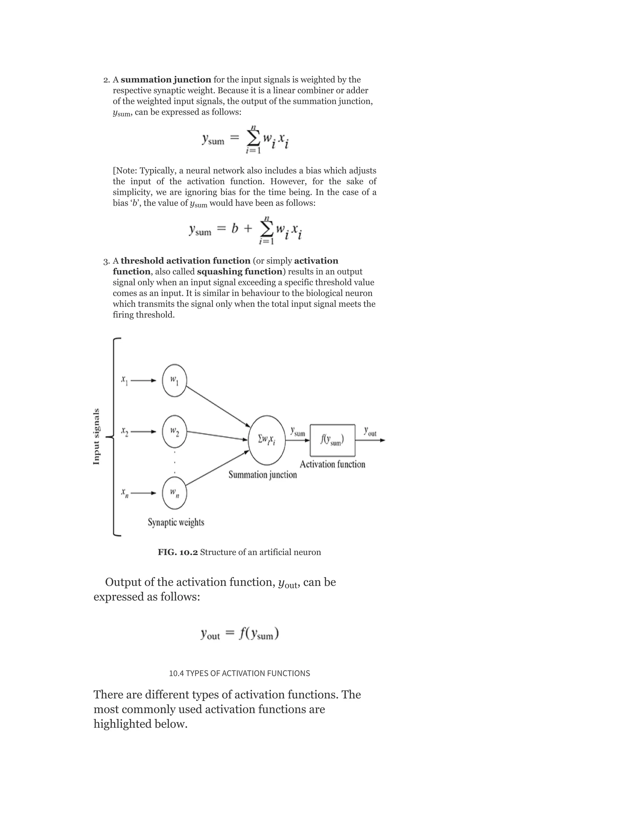
Basics of Neural Network: Understanding biological
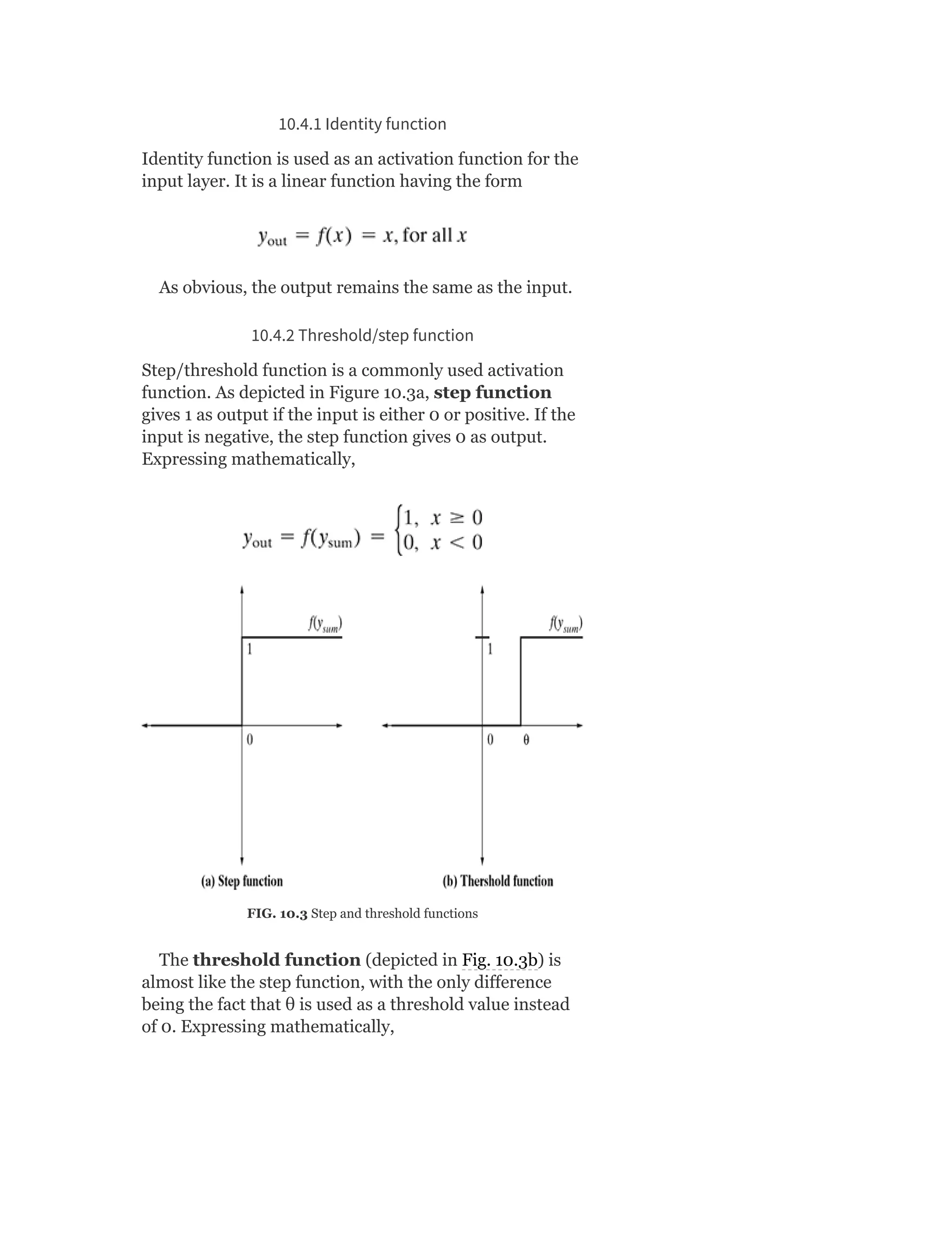
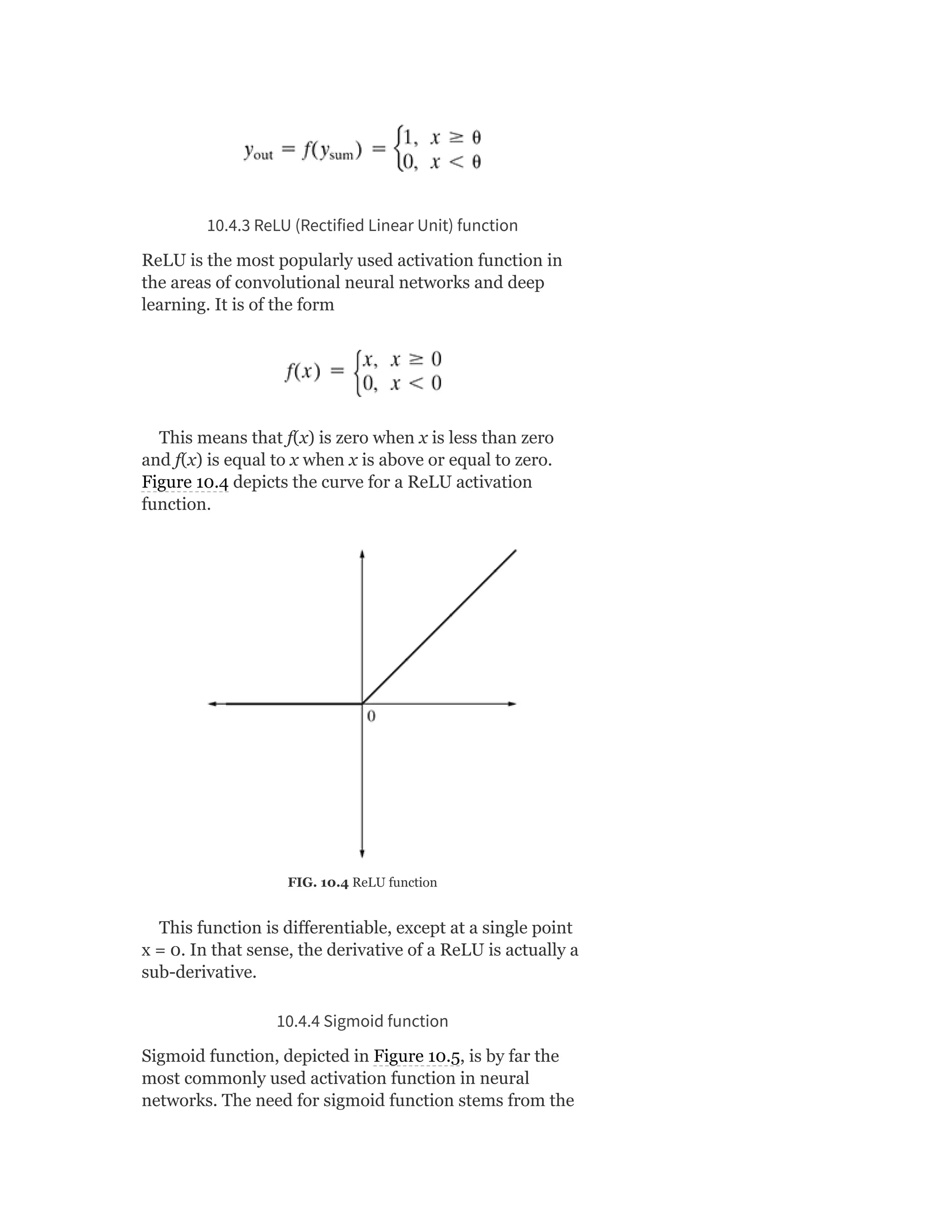
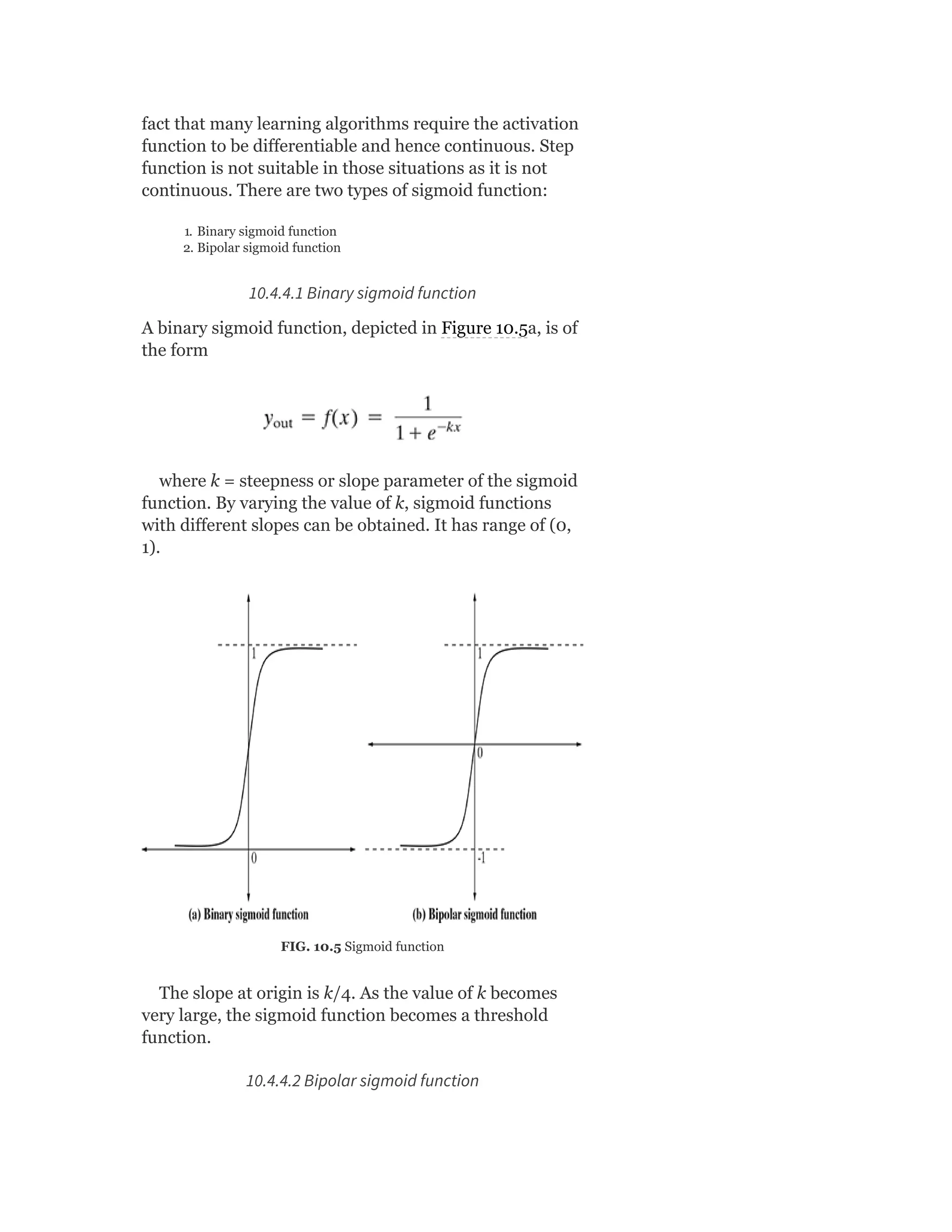
neuron and artificial neuron; types of activation
functions; early implementations – McCulloch Pitt’s,
Rosenblatt’s Perceptron, ADALINE; architectures of
neural network; learning process in ANN;
backpropagation
Other types of learning: Representation learning;
active learning; instance-based learning; association rule
learning; ensemble learning; regularization
Machine Learning Live Case Studies
[8 Lectures]](https://image.slidesharecdn.com/mlsaikatdutt-221115120700-3df1a1af/75/ML_saikat-dutt-pdf-24-2048.jpg)


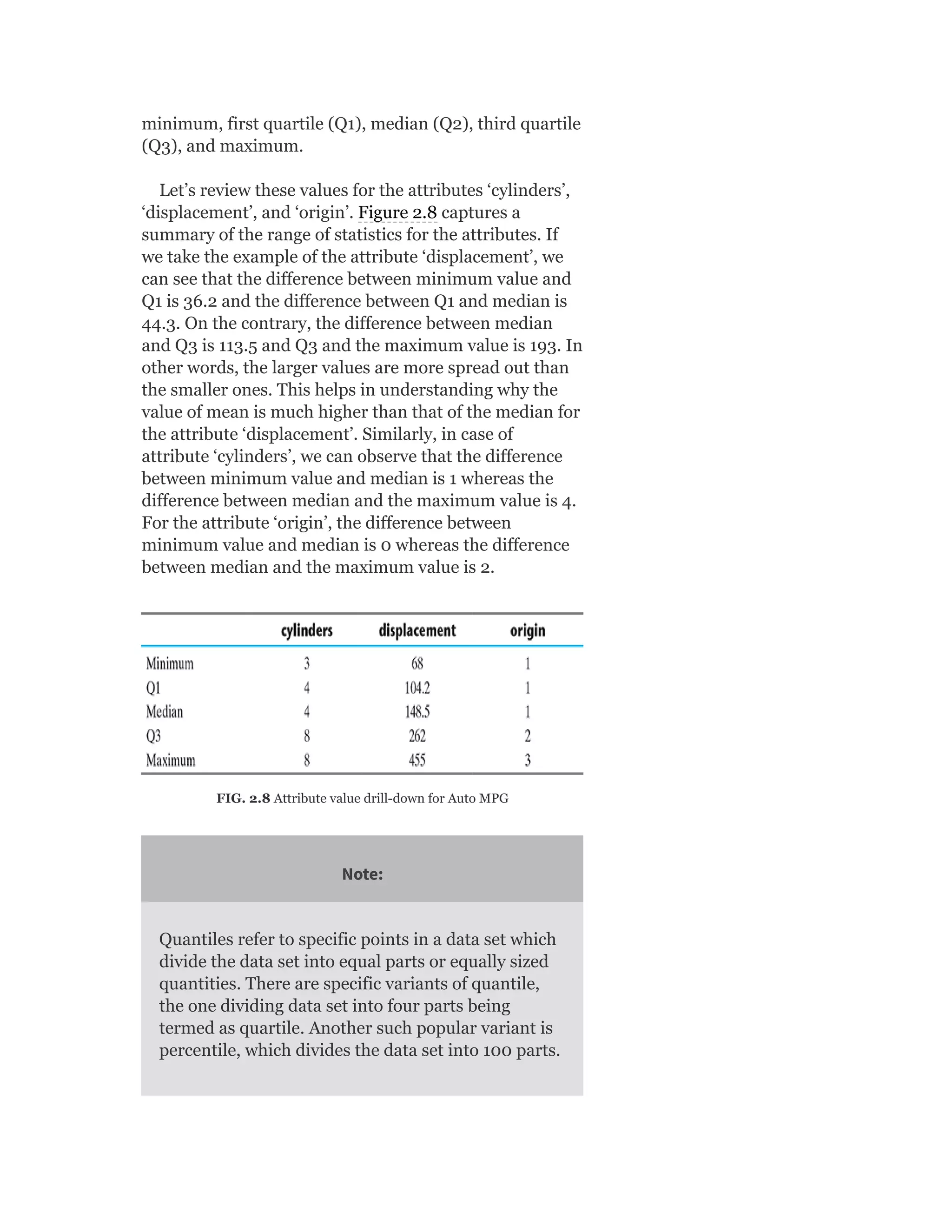
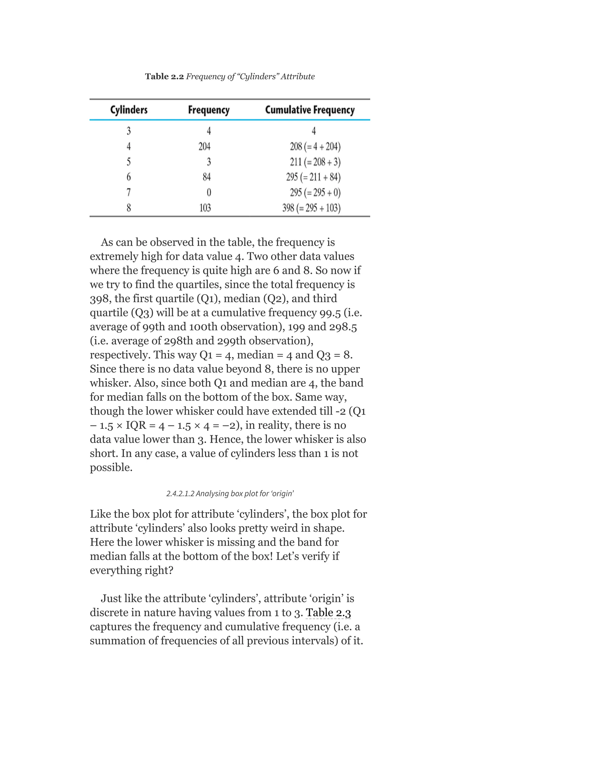
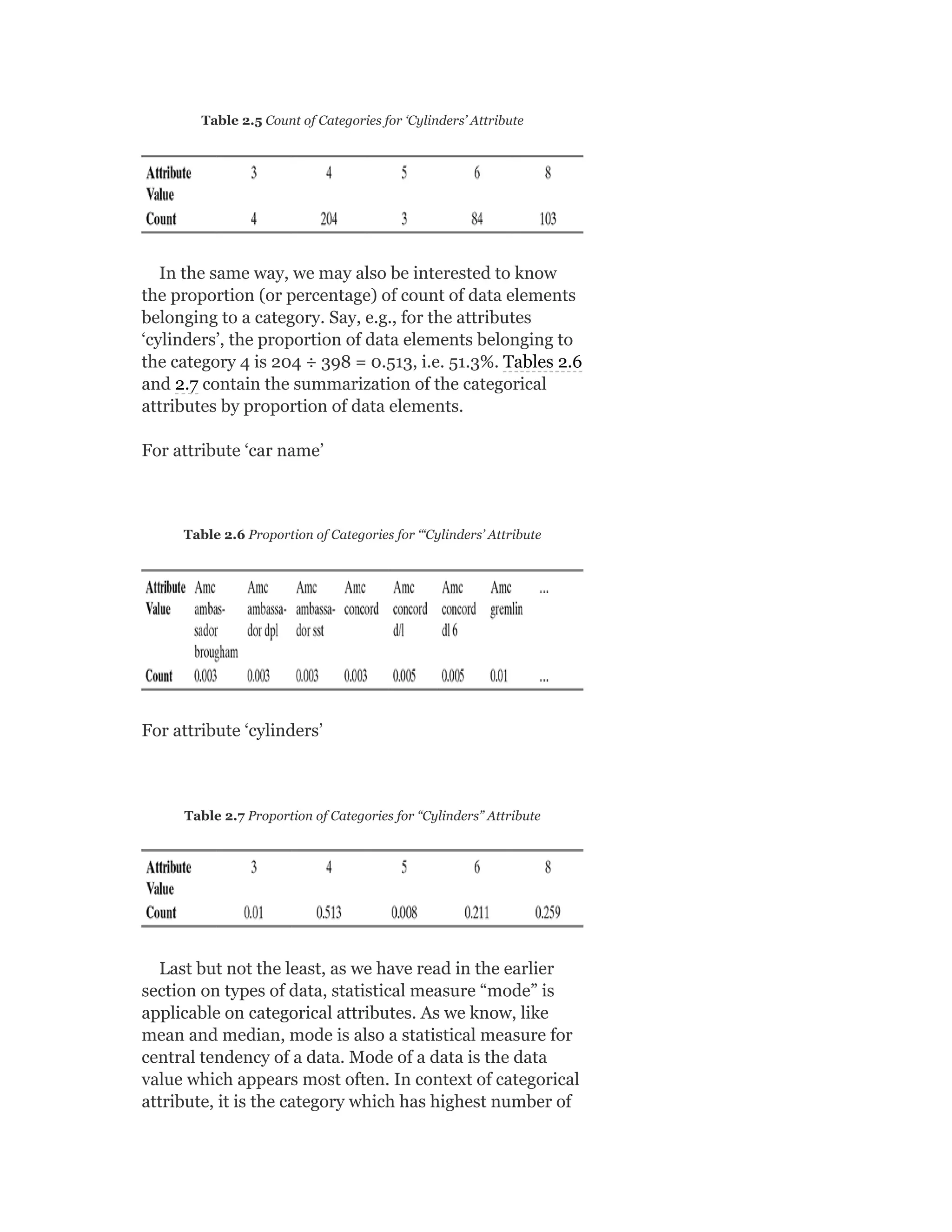
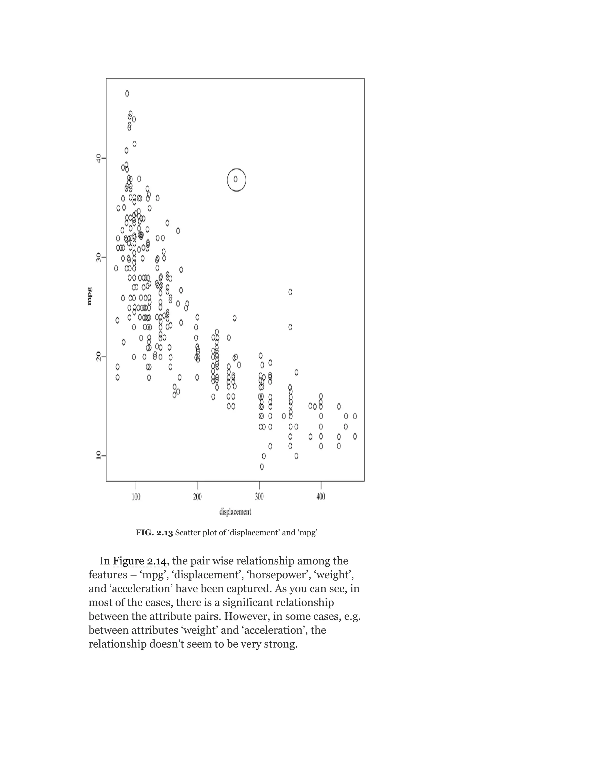
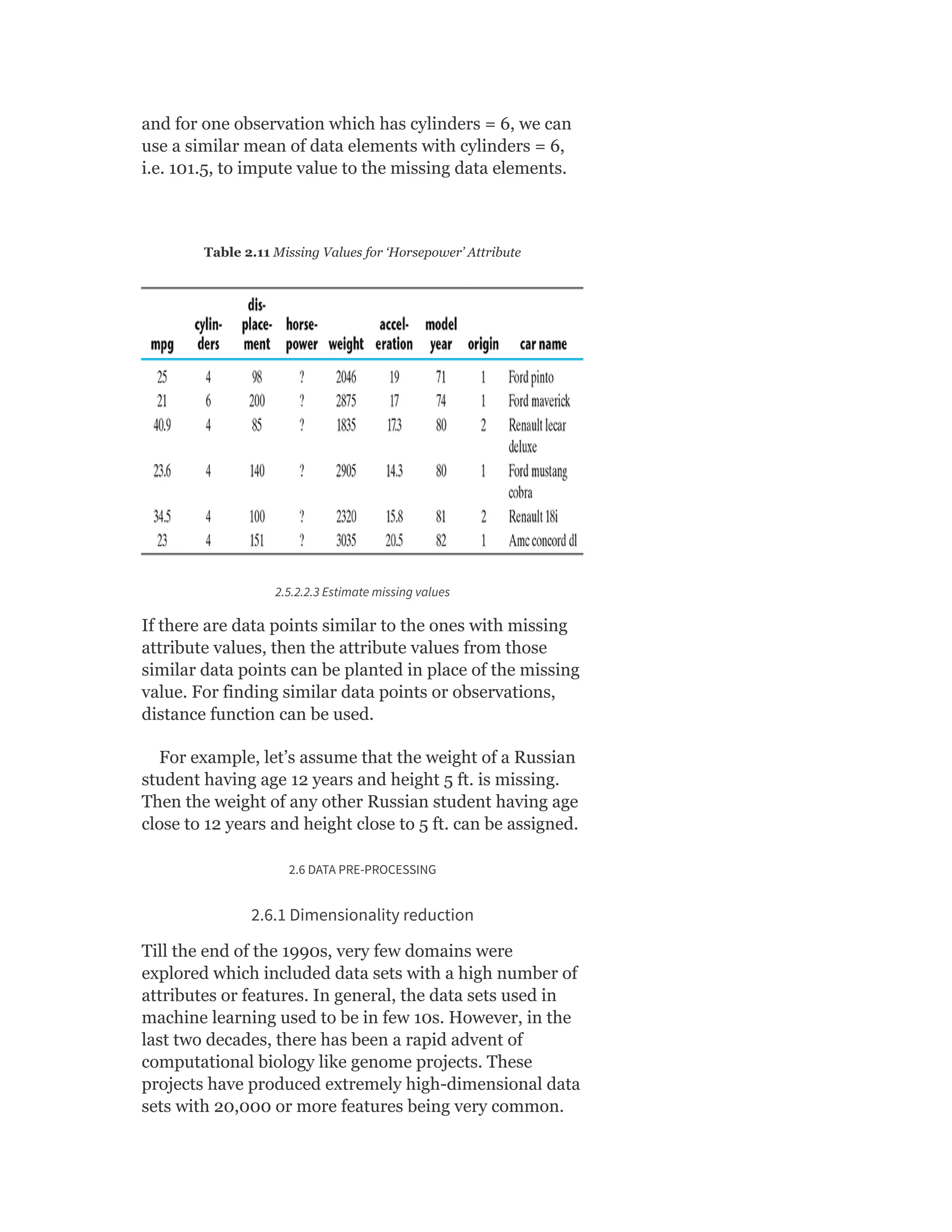
![Table 2.3 Frequency of “Origin” Attribute
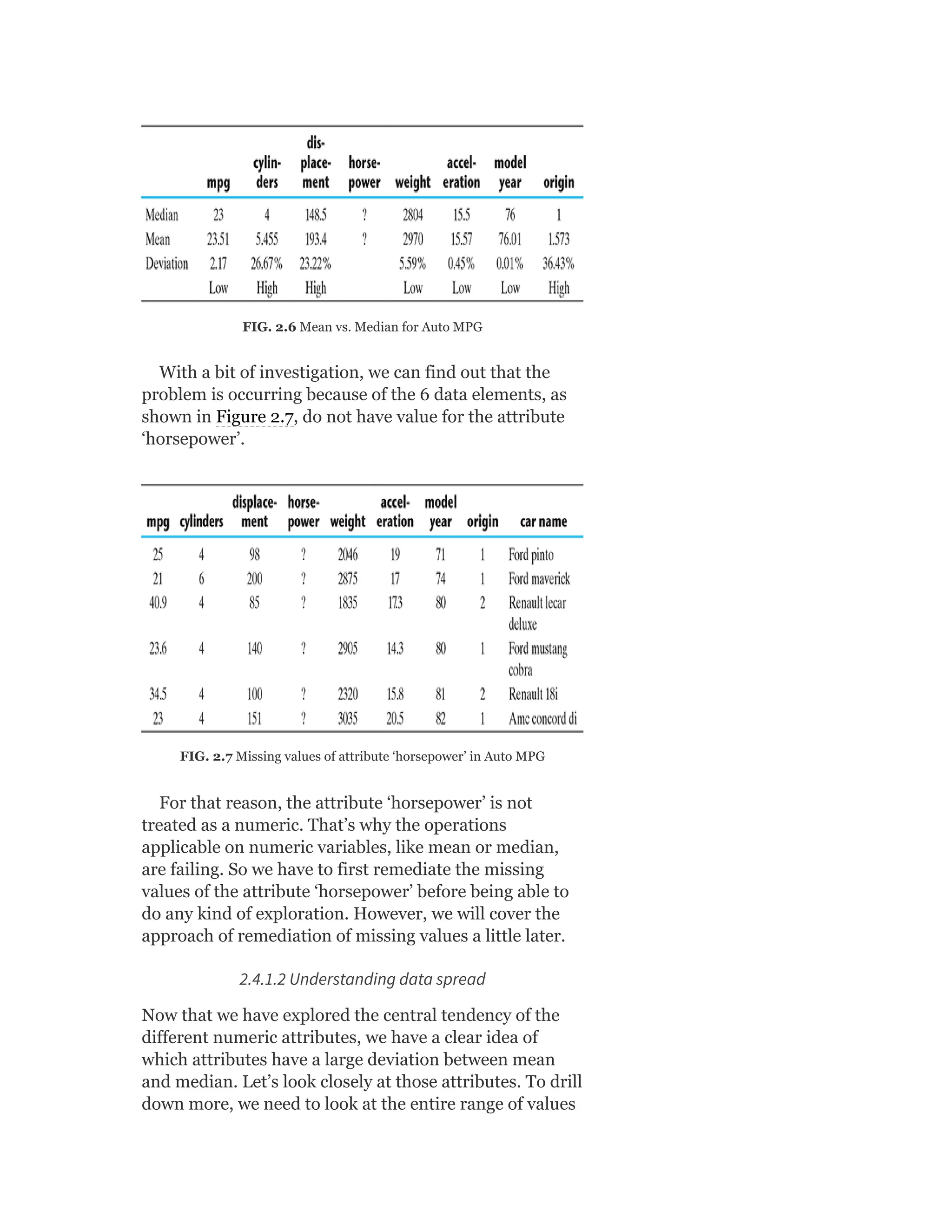
As can be observed in the table, the frequency is
extremely high for data value 1. Since the total frequency
is 398, the first quartile (Q1), median (Q2), and third
quartile (Q3) will be at a cumulative frequency 99.5 (i.e.
average of 99th and 100th observation), 199 and 298.5
(i.e. average of 298th and 299th observation),
respectively. This way Q1 = 1, median = 1, and Q3 = 2.
Since Q1 and median are same in value, the band for
median falls on the bottom of the box. There is no data
value lower than Q1. Hence, the lower whisker is
missing.
2.4.2.1.3 Analysing box plot for ‘displacement’
The box plot for the attribute ‘displacement’ looks better
than the previous box plots. However, still, there are few
small abnormalities, the cause of which needs to be
reviewed. Firstly, the lower whisker is much smaller than
an upper whisker. Also, the band for median is closer to
the bottom of the box.
Let’s take a closer look at the summary data of the
attribute ‘displacement’. The value of first quartile, Q1 =
104.2, median = 148.5, and third quartile, Q3 = 262.
Since (median – Q1) = 44.3 is greater than (Q3 –
median) = 113.5, the band for the median is closer to the
bottom of the box (which represents Q1). The value of
IQR, in this case, is 157.8. So the lower whisker can be 1.5
times 157.8 less than Q1. But minimum data value for the
attribute ‘displacement’ is 68. So, the lower whisker at
15% [(Q1 – minimum)/1.5 × IQR = (104.2 – 68) / (1.5 ×
157.8) = 15%] of the permissible length. On the other
hand, the maximum data value is 455. So the upper
whisker is 81% [(maximum – Q3)/1.5 × IQR = (455 –
262) / (1.5 × 157.8) = 81%] of the permissible length.
This is why the upper whisker is much longer than the
lower whisker.](https://image.slidesharecdn.com/mlsaikatdutt-221115120700-3df1a1af/75/ML_saikat-dutt-pdf-88-2048.jpg)
![2.4.2.1.4 Analysing box plot for ‘model Year’
The box plot for the attribute ‘model. year’ looks perfect.
Let’s validate is it really what expected to be.
For the attribute ‘model.year’:
First quartile, Q1 = 73
Median, Q2 = 76
Third quartile, Q3 = 79
So, the difference between median and Q1 is exactly
equal to Q3 and median (both are 3). That is why the
band for the median is exactly equidistant from the
bottom and top of the box.
I QR = Q3 9 Q1 = 7 9 - 7 3 = 6
Difference between Q1 and minimum data value (i.e. 70)
is also same as maximum data value (i.e. 82) and Q3
(both are 3). So both lower and upper whiskers are
expected to be of the same size which is 33% [3 / (1.5 ×
6)] of the permissible length.
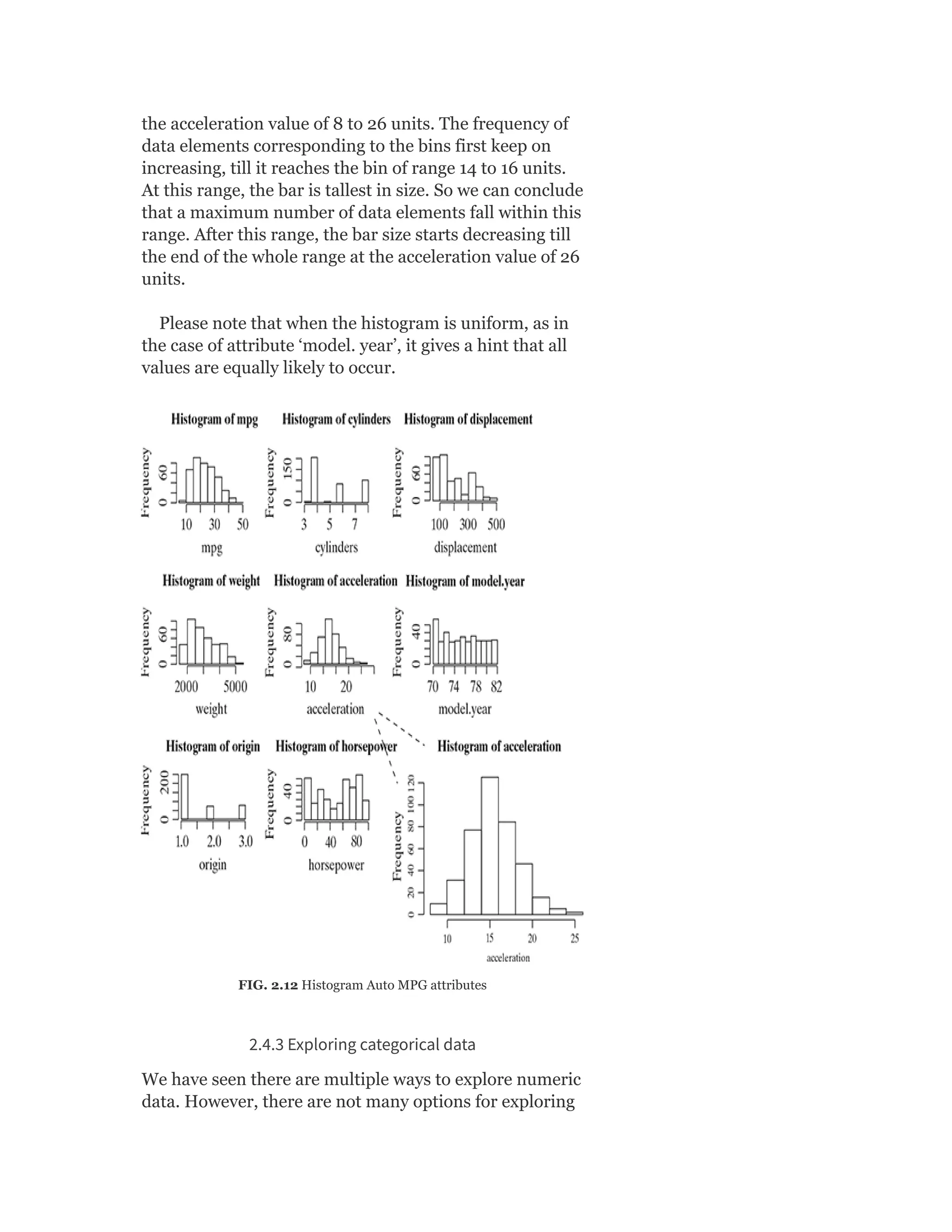
2.4.2.2 Histogram
Histogram is another plot which helps in effective
visualization of numeric attributes. It helps in
understanding the distribution of a numeric data into
series of intervals, also termed as ‘bins’. The important
difference between histogram and box plot is
The focus of histogram is to plot ranges of data values (acting as
‘bins’), the number of data elements in each range will depend on the
data distribution. Based on that, the size of each bar corresponding
to the different ranges will vary.
The focus of box plot is to divide the data elements in a data set into
four equal portions, such that each portion contains an equal
number of data elements.
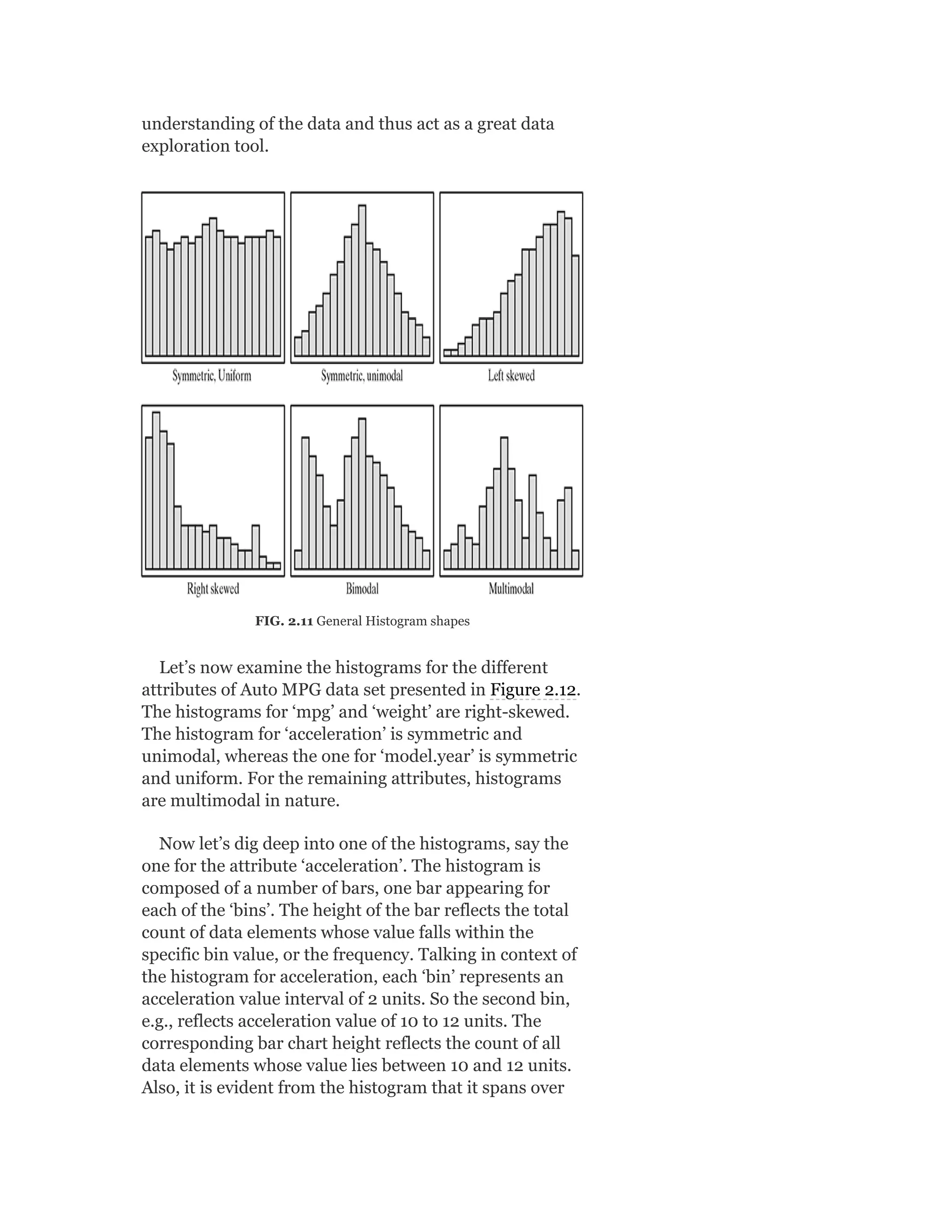
Histograms might be of different shapes depending on
the nature of the data, e.g. skewness. Figure 2.11 provides
a depiction of different shapes of the histogram that are
generally created. These patterns give us a quick](https://image.slidesharecdn.com/mlsaikatdutt-221115120700-3df1a1af/75/ML_saikat-dutt-pdf-89-2048.jpg)


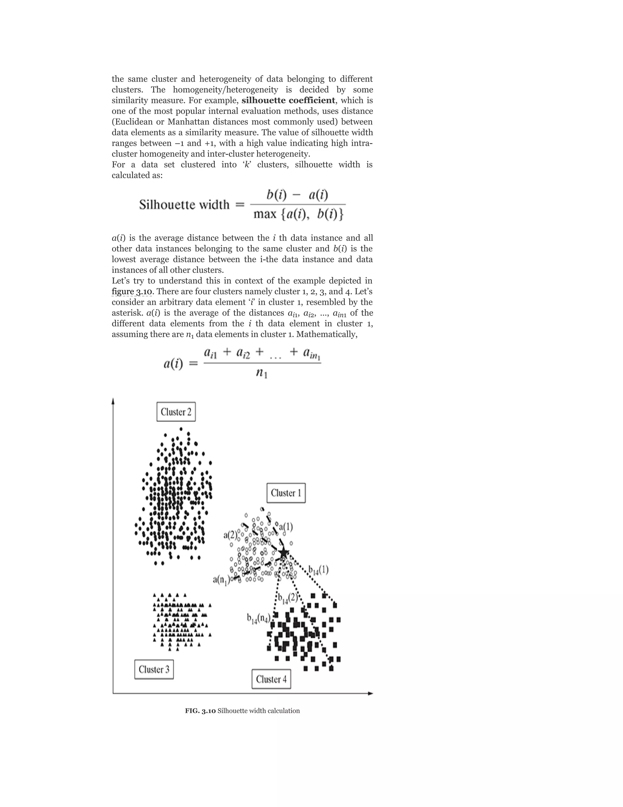
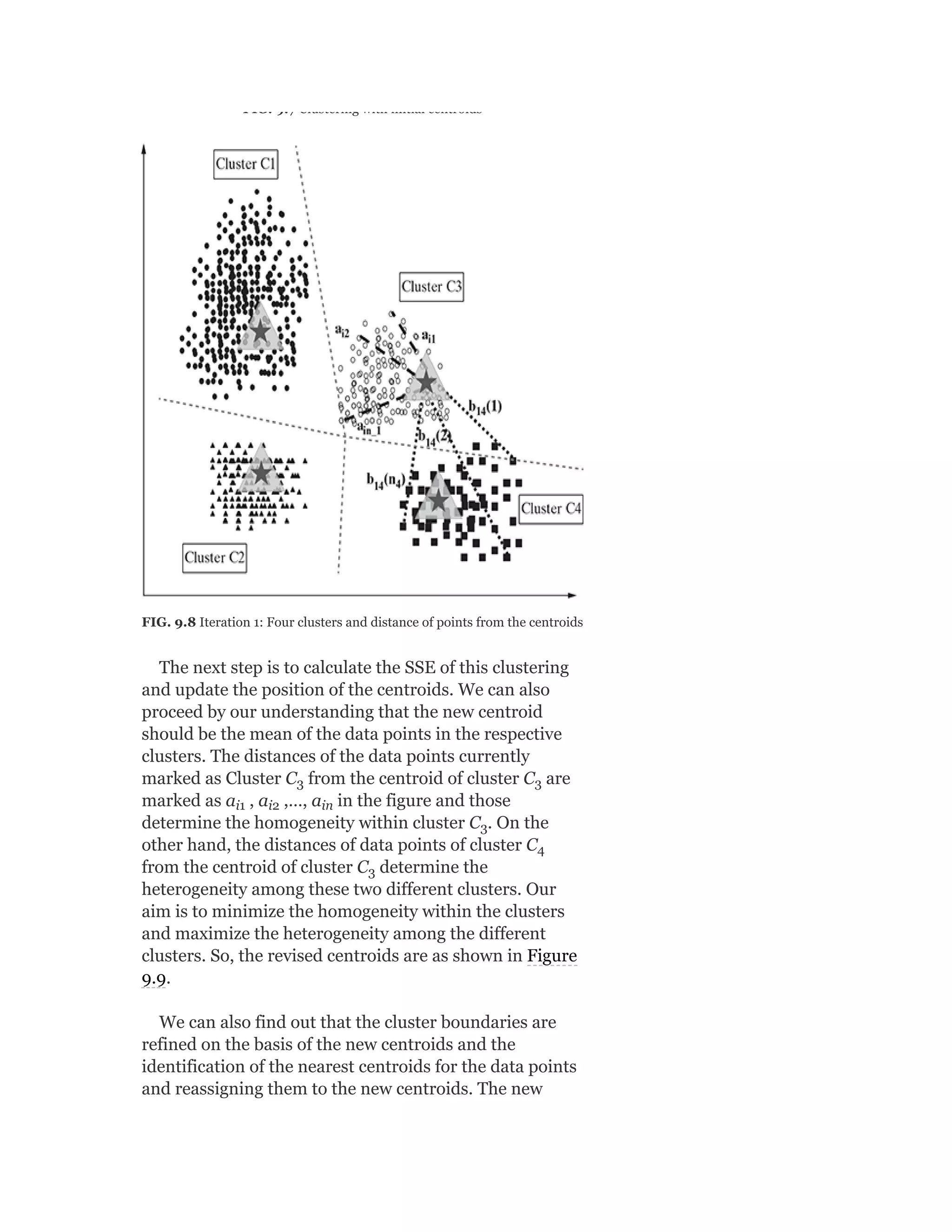
![In the same way, let’s calculate the distance of an arbitrary data
element ‘i’ in cluster 1 with the different data elements from another
cluster, say cluster 4 and take an average of all those distances.
Hence,
where n is the total number of elements in cluster 4. In the same
way, we can calculate the values of b (average) and b (average). b
(i) is the minimum of all these values. Hence, we can say that,
b(i) = minimum [b (average), b (average), b (average)]
2. External evaluation
In this approach, class label is known for the data set subjected to
clustering. However, quite obviously, the known class labels are not
a part of the data used in clustering. The cluster algorithm is
assessed based on how close the results are compared to those
known class labels. For example, purity is one of the most popular
measures of cluster algorithms – evaluates the extent to which
clusters contain a single class.
For a data set having ‘n’ data instances and ‘c’ known class labels
which generates ‘k’ clusters, purity is measured as:
3.6 IMPROVING PERFORMANCE OF A MODEL
Now we have almost reached the end of the journey of
building learning models. We have got some idea about
what modelling is, how to approach about it to solve a
learning problem and how to measure the success of our
model. Now comes a million dollar question. Can we
improve the performance of our model? If so, then what
are the levers for improving the performance? In fact,
even before that comes the question of model selection –
which model should be selected for which machine
learning task? We have already discussed earlier that the
model selection is done one several aspects:
1. Type of learning the task in hand, i.e. supervised or
unsupervised
2. Type of the data, i.e. categorical or numeric
3. Sometimes on the problem domain
4. Above all, experience in working with different models to solve
problems of diverse domains
So, assuming that the model selection is done, what
are the different avenues to improve the performance of
models?
4
12 13
12 13 14](https://image.slidesharecdn.com/mlsaikatdutt-221115120700-3df1a1af/75/ML_saikat-dutt-pdf-142-2048.jpg)


![advisable to remove the mean of a data attribute,
especially when the data set is sparse (as in case of text
data), SVD is a good choice for dimensionality reduction
in those situations.
SVD of a data matrix is expected to have the properties
highlighted below:
1. Patterns in the attributes are captured by the right-singular
vectors, i.e. the columns of V.
2. Patterns among the instances are captured by the left-singular,
i.e. the columns of U.
3. Larger a singular value, larger is the part of the matrix A that it
accounts for and its associated vectors.
4. New data matrix with ‘k’ attributes is obtained using the
equation
D = D × [v , v , … , v ]
Thus, the dimensionality gets reduced to k
SVD is often used in the context of text data.
4.2.2.3 Linear Discriminant Analysis
Linear discriminant analysis (LDA) is another commonly
used feature extraction technique like PCA or SVD. The
objective of LDA is similar to the sense that it intends to
transform a data set into a lower dimensional feature
space. However, unlike PCA, the focus of LDA is not to
capture the data set variability. Instead, LDA focuses on
class separability, i.e. separating the features based on
class separability so as to avoid over-fitting of the
machine learning model.
Unlike PCA that calculates eigenvalues of the
covariance matrix of the data set, LDA calculates
eigenvalues and eigenvectors within a class and inter-
class scatter matrices. Below are the steps to be followed:
1. Calculate the mean vectors for the individual classes.
2. Calculate intra-class and inter-class scatter matrices.
3. Calculate eigenvalues and eigenvectors for S and S , where
S is the intra-class scatter matrix and S is the inter-class
scatter matrix
where, m is the mean vector of the i-th class
1 2 k
W B
W B
i
′
-1](https://image.slidesharecdn.com/mlsaikatdutt-221115120700-3df1a1af/75/ML_saikat-dutt-pdf-163-2048.jpg)


![This means that if we combine our prior knowledge
with the actual test results then there is only about a 3%
chance of emails actually being spam if the sender name
contains the terms ‘bulk’ or ‘mass’. This is significantly
lower than the earlier assumption of 80% chance and
thus calls for additional checks before someone starts
deleting such emails based on only this flag.
Details of the practice application of Bayes theorem in
machine learning is discussed in Chapter 6.
5.4 RANDOM VARIABLES
Let’s take an example of tossing a coin once. We can
associate random variables X and Y as
X(H) = 1, X(T) = 0, which means this variable is
associated with the outcome of the coin facing head.
Y(H) = 0, Y(T) = 1, which means this variable is
associated with the outcome of the coin facing tails.
Here in the sample space S which is the outcome
related to tossing the coin once, random variables
represent the single-valued real function [X(ζ)] that
assigns a real number, called its value to each sample
point of S. A random variable is not a variable but is a
function. The sample space S is called the domain of
random variable X and the collection of all the numbers,
i.e. values of X(ζ), is termed the range of the random
variable.
We can define the event (X = x) where x is a fixed real
number as
(X = x) = { ζ:X(ζ) = x }
Accordingly, we can define the following events for
fixed numbers x, x , and x :
(X ≤ x) = { ζ:X(ζ) ≤ x }
(X > x) = { ζ:X(ζ) > x }
(x < X ≤ x ) = { ζ:x < X(ζ) ≤ x }
1 2
1 2 1 2](https://image.slidesharecdn.com/mlsaikatdutt-221115120700-3df1a1af/75/ML_saikat-dutt-pdf-191-2048.jpg)
![5.5.3 The multinomial and multinoulli distributions
The binomial distribution can be used to model the
outcomes of coin tosses, or for experiments where the
outcome can be either success or failure. But to model
the outcomes of tossing a K-sided die, or for experiments
where the outcome can be multiple, we can use the
multinomial distribution. This is defined as: let x = (x ,
…, x ) be a random vector, where x is the number of
times side j of the die occurs. Then x has the following
pmf:
where, x + x +….. x = n and
the multinomial coefficient is defined as
and the summation is over the set of all non-negative
integers x , x , … . x whose sum is n.
Now consider a special case of n = 1, which is like
rolling a K-sided dice once, so x will be a vector of 0s and
1s (a bit vector), in which only one bit can be turned on.
This means, if the dice shows up face k, then the k’th bit
will be on. We can consider x as being a scalar categorical
random variable with K states or values, and x is its
dummy encoding with x = [Π(x = 1), …,Π(x = K)].
For example, if K = 3, this states that 1, 2, and 3 can be
encoded as (1, 0, 0), (0, 1, 0), and (0, 0, 1). This is also
called a one-hot encoding, as we interpret that only
one of the K ‘wires’ is ‘hot’ or on. This very common
special case is known as a categorical or discrete
distribution and because of the analogy with the
Binomial/ Bernoulli distinction, Gustavo Lacerda
suggested that this is called the multinoulli
distribution.
1
K j
1 2 K
1 2 k](https://image.slidesharecdn.com/mlsaikatdutt-221115120700-3df1a1af/75/ML_saikat-dutt-pdf-200-2048.jpg)
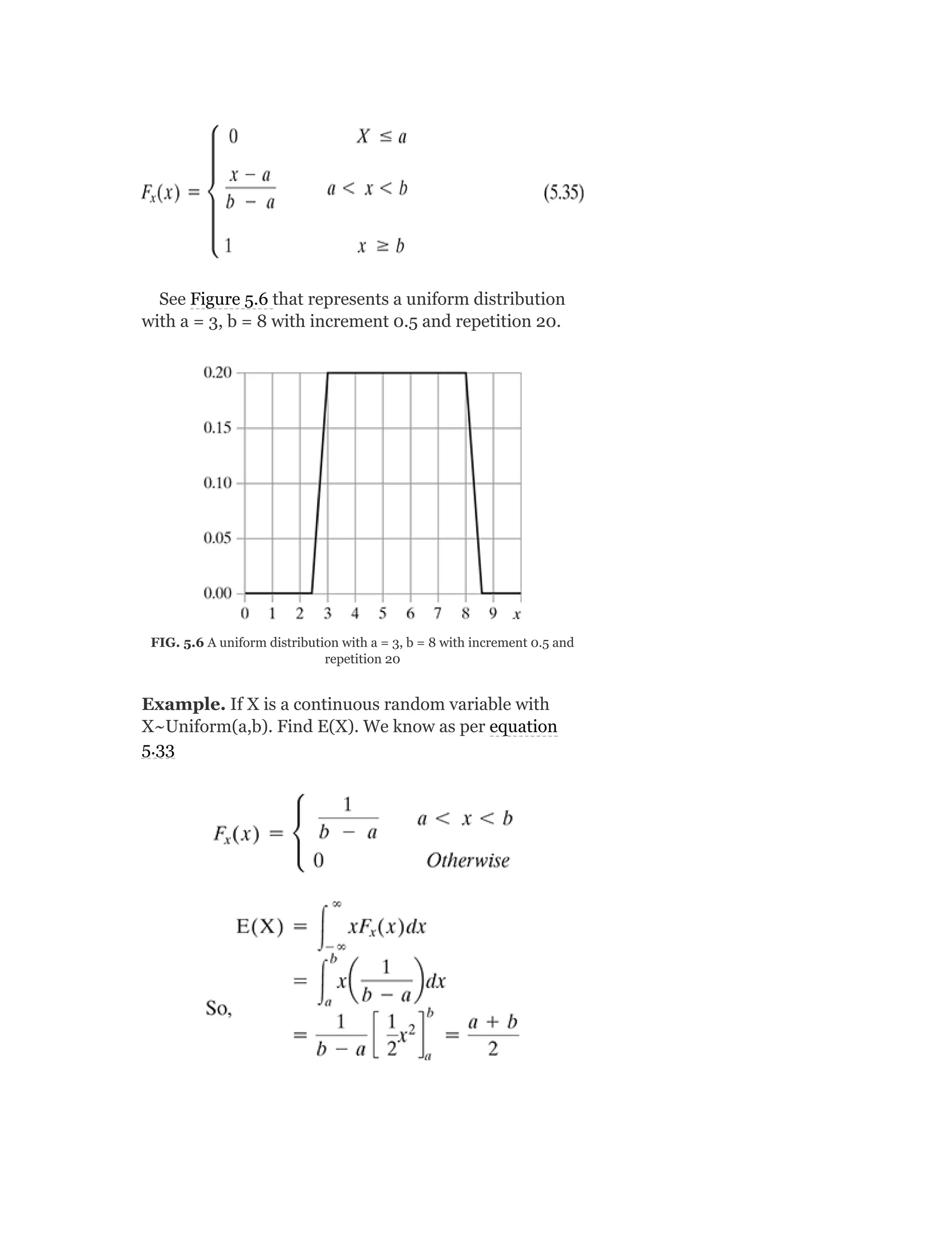
![This is also corroborated by the fact that because X is
uniformly distributed over the interval [a, b] we can
expect the mean to be at the middle point, E(X) =
The mean and variance of a uniform random variable
X are
This is a useful distribution when we don’t have any
prior knowledge of the actual pdf and all continuous
values in the same range seems to be equally likely.
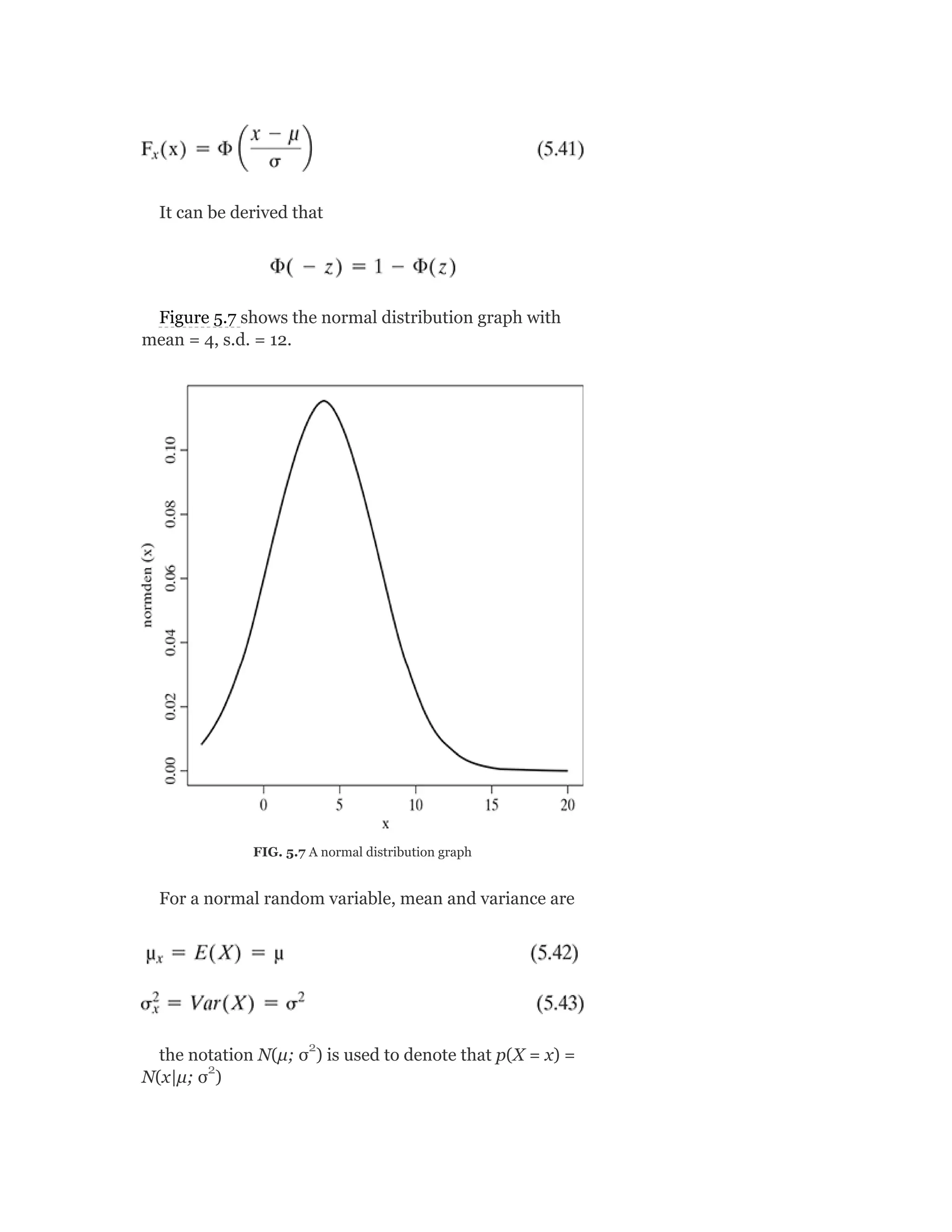
5.6.2 Gaussian (normal) distribution
The most widely used distribution in statistics and
machine learning is the Gaussian or normal distribution.
Its pdf is given by
and the corresponding cdf looks like
For easier reference a function Φ(z) is defined as
Which will help us evaluate the value of F (x) which
can be written as
x](https://image.slidesharecdn.com/mlsaikatdutt-221115120700-3df1a1af/75/ML_saikat-dutt-pdf-204-2048.jpg)

![Few important properties of joint cdf of two random
variables which are similar to that of the cdf of single
random variable are
1. 0 ≤ F (x, y) ≤ 1
If x ≤ x and y ≤ y , then
F (x , y ) ≤ F (x , y ) ≤ F (x , y )
2. F (x , y ) ≤ F (x , y ) ≤ F (x , y )
3.
4.
5.
6. P (x < X ≤ x , Y ≤ y) = F (x , y)-F (x , y)
P (X < x, y < Y ≤ y ) = F (x, y )-F (x, y )
5.7.3 Joint probability mass functions
For the discrete bivariate random variable (X, Y) if it
takes the values (x , y ) for certain allowable integers I
and j, then the joint probability mass function (joint
pmf) of (X, Y) is given by
Few important properties of p (x , y ) are
1. 0 ≤ p (x , y ) ≤ 1
2.
3. P[(X, Y) ∈ A] = Ʃ (x , y ) ∈ R Ʃ p (x , y ), where the summation
is done over the points (x , y ) in the range space R .
The joint cdf of a discrete bivariate random variable
(X, Y) is given by
XY
1 2 1 2
XY 1 1 XY 2 1 XY 2 2
XY 1 1 XY 1 2 XY 2 2
1 2 XY 2 XY 1
1 2 XY 2 XY 1
i j
XY i j
XY i j
i j A XY i j
i j A](https://image.slidesharecdn.com/mlsaikatdutt-221115120700-3df1a1af/75/ML_saikat-dutt-pdf-210-2048.jpg)
![The outcomes of a Random Variable weighted by their probability is
Expectation, E(X).
The difference between Expectation of a squared Random Variable
and the Expectation of that Random Variable squared is Variance:
E(X ) − E(X) .
Covariance, E(XY) − E(X)E(Y) is the same as Variance, but here two
Random Variables are compared, rather than a single Random
Variable against itself.
Correlation, Corr (X, Y) = is the
Covariance normalized.
Few important properties of correlation are
1. −1 ≤ corr [X, Y] ≤ 1. Hence, in a correlation matrix, each entry
on the diagonal is 1, and the other entries are between -1 and 1.
2. corr [X, Y] = 1 if and only if Y = aX + b for some parameters a
and b, i.e., if there is a linear relationship between X and Y.
3. From property 2 it may seem that the correlation coefficient is
related to the slope of the regression line, i.e., the coefficient a in
the expression Y = aX + b. However, the regression coefficient is
in fact given by a = cov[X, Y] /var [X]. A better way to interpret
the correlation coefficient is as a degree of linearity.
5.8 CENTRAL LIMIT THEOREM
This is one of the most important theorems in
probability theory. It states that if X ,… X is a sequence
of independent identically distributed random variables
and each having mean μ and variance σ and
As n → ∞ (meaning for a very large but finite set) then
Z tends to the standard normal.
Or
1 n
n
2 2
2](https://image.slidesharecdn.com/mlsaikatdutt-221115120700-3df1a1af/75/ML_saikat-dutt-pdf-214-2048.jpg)

![8. If X is a continuous random variable with pdf
9. If X~Uniform and Y = sin(X), then find f (y).
10. If X is a random variable with CDF
1. What kind of random variable is X: discrete, continuous,
or mixed?
2. Find the PDF of X, fX(x).
3. Find E(e ).
4. Find P(X = 0|X≤0.5).
11. There are two random variables X and Y with joint PMF given in
Table below
1. Find P(X≤2, Y≤4).
2. Find the marginal PMFs of X and Y.
3. Find P(Y = 2|X = 1).
4. Are X and Y independent?
12. There is a box containing 40 white shirts and 60 black shirts. If
we choose 10 shirts (without replacement) at random, then find
the joint PMF of X and Y where X is the number of white shirts
and Y is the number of black shirts.
13. If X and Y are two jointly continuous random variables with
joint PDF
1. Find f (x) and f (y).
2. Are X and Y independent to each other?
3. Find the conditional PDF of X given Y = y, f (x|y).
4. Find E[X|Y = y], for 0 ≤ y ≤ 1.
5. Find Var(X|Y = y), for 0 ≤ y ≤ 1.
14. There are 100 men on a ship. If X is the weight of the ith man
on the ship and Xi’s are independent and identically distributed
Y
X Y
X|Y
i
X](https://image.slidesharecdn.com/mlsaikatdutt-221115120700-3df1a1af/75/ML_saikat-dutt-pdf-226-2048.jpg)


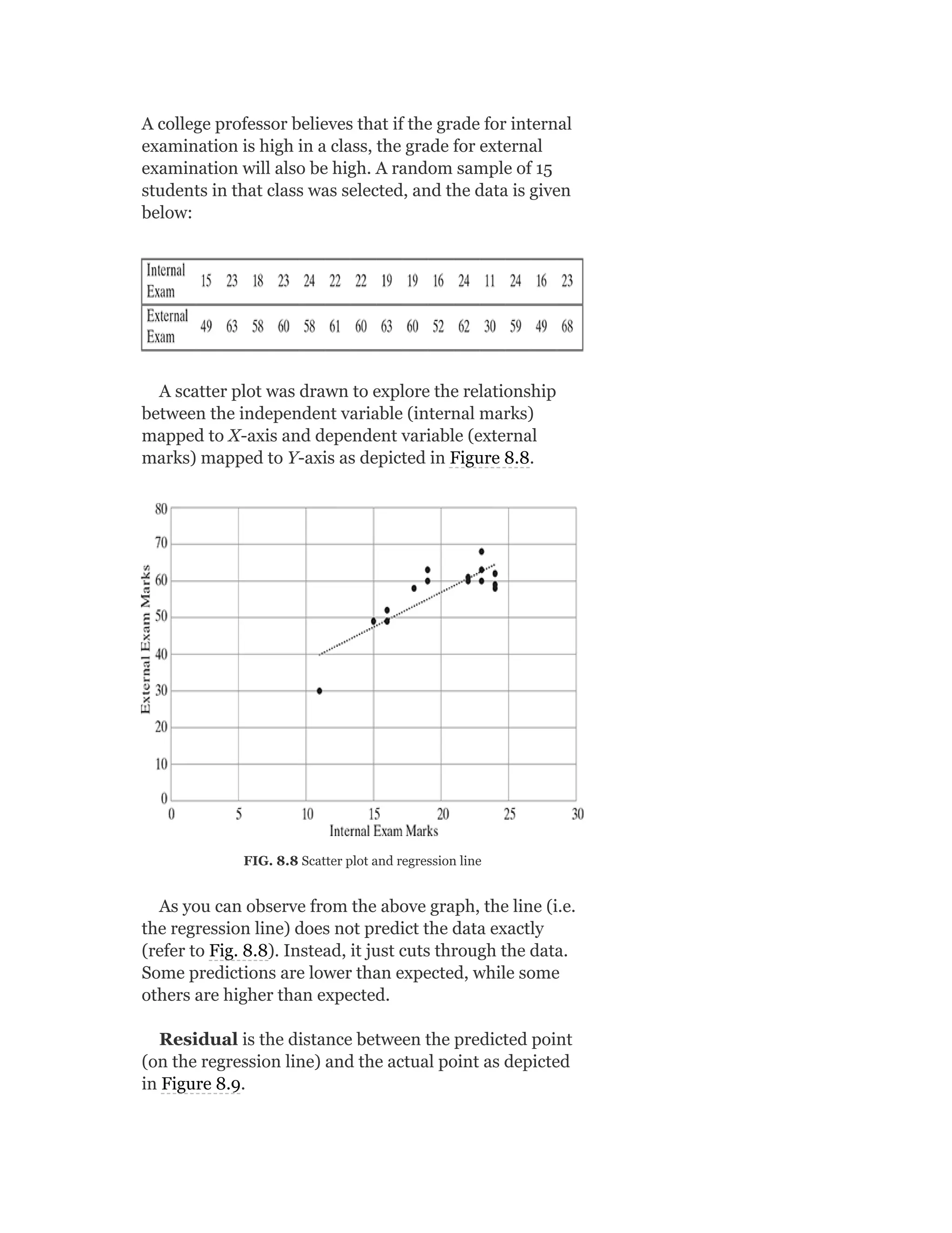


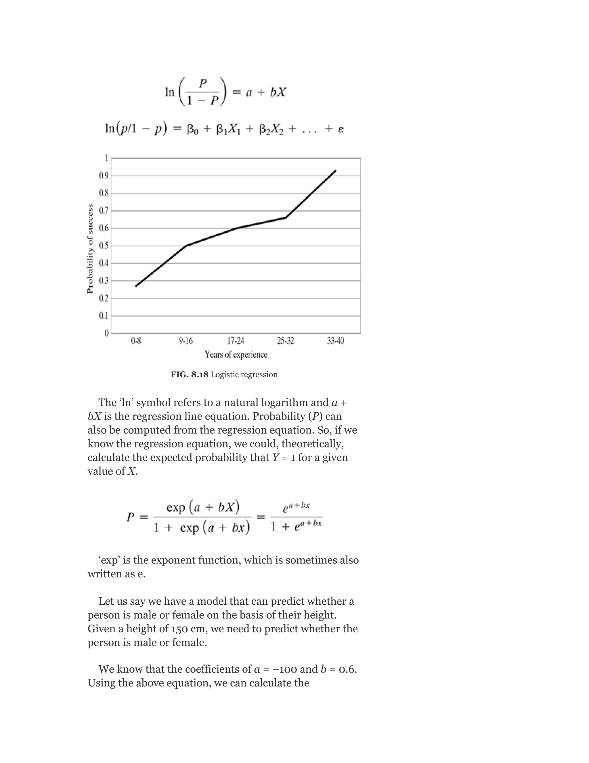
![probability of male given a height of 150 cm or more
formally P(male|height = 150).
y = e^(a + b × X)/(1 + e^(a + b × X))
y = exp ( −100 + 0.6 × 150)/(1 + EXP( −100 + 0.6 × X)
y = 0.000046
or a probability of near zero that the person is a male.
Assumptions in logistic regression
The following assumptions must hold when building a
logistic regression model:
There exists a linear relationship between logit function and
independent variables
The dependent variable Y must be categorical (1/0) and take binary
value, e.g. if pass then Y = 1; else Y = 0
The data meets the ‘iid’ criterion, i.e. the error terms, ε, are
independent from one another and identically distributed
The error term follows a binomial distribution [n, p]
n = # of records in the data
p = probability of success (pass, responder)
8.3.8 Maximum Likelihood Estimation
The coefficients in a logistic regression are estimated
using a process called Maximum Likelihood Estimation
(MLE). First, let us understand what is likelihood
function before moving to MLE. A fair coin outcome flips
equally heads and tails of the same number of times. If
we toss the coin 10 times, it is expected that we get five
times Head and five times Tail.
Let us now discuss about the probability of getting
only Head as an outcome; it is 5/10 = 0.5 in the above
case. Whenever this number (P) is greater than 0.5, it is
said to be in favour of Head. Whenever P is lesser than
0.5, it is said to be against the outcome of getting Head.
Let us represent ‘n’ flips of coin as X , X , X ,…, X .
Now X can take the value of 1 or 0.
X = 1 if Head is the outcome
X = 0 if Tail is the outcome
1 2 3 n
i
i
i](https://image.slidesharecdn.com/mlsaikatdutt-221115120700-3df1a1af/75/ML_saikat-dutt-pdf-343-2048.jpg)


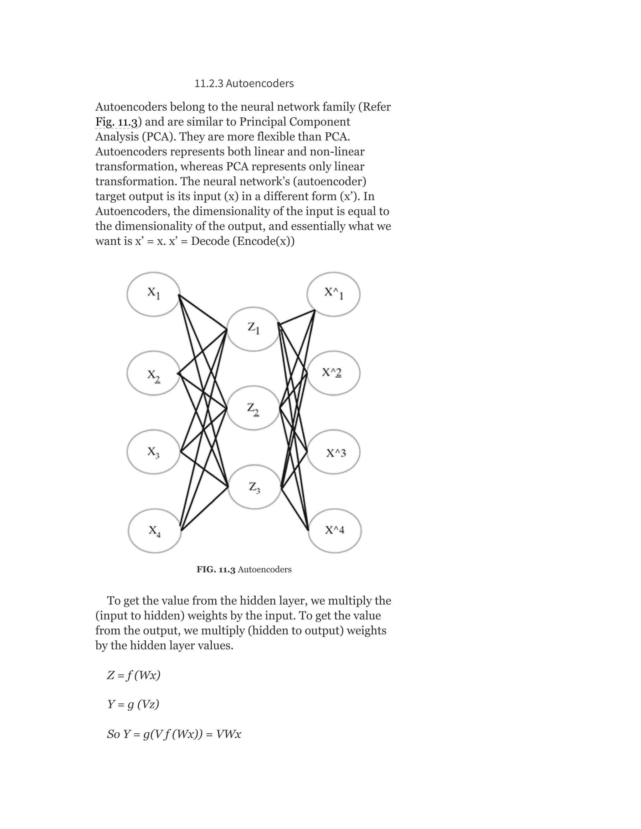
![So Objective Function J = ∑ [Xn – VWx (n)]
Heuristics for Autoencoders
Autoencoder training algorithm can be summarized as
below:
For each input x
1. Do a feed-forward pass to compute activations at all hidden
layers, then at the output layer to obtain an output X
2. Measure the deviation X from the input X
3. Backpropagate the error through the net and perform weight
updates.
11.2.4 Various forms of clustering
Refer chapter 9 titled ‘Unsupervised Learning’ to know
more about various forms of Clustering.
11.3 ACTIVE LEARNING
Active learning is a type of semi-supervised learning in
which a learning algorithm can interactively query
(question) the user to obtain the desired outputs at new
data points.
Let P be the population set of all data under
consideration. For example, all male students studying in
a college are known to have a particularly exciting study
pattern.
During each iteration, I, P (total population) is broken
up into three subsets.
1. P(K, i): Data points where the label is known (K).
2. P(U, i): Data points where the label is unknown (U)
3. P(C, i): A subset of P(U, i)that is chosen (C) to be labelled.
Current research in this type of active learning
concentrates on identifying the best method P(C, i) to
chose (C) the data points.
11.3.1 Heuristics for active learning
1. Start with a pool of unlabelled data P(U, i)
2. Pick a few points at random and get their labels P(C, i)
3. Repeat
2
′
′](https://image.slidesharecdn.com/mlsaikatdutt-221115120700-3df1a1af/75/ML_saikat-dutt-pdf-436-2048.jpg)


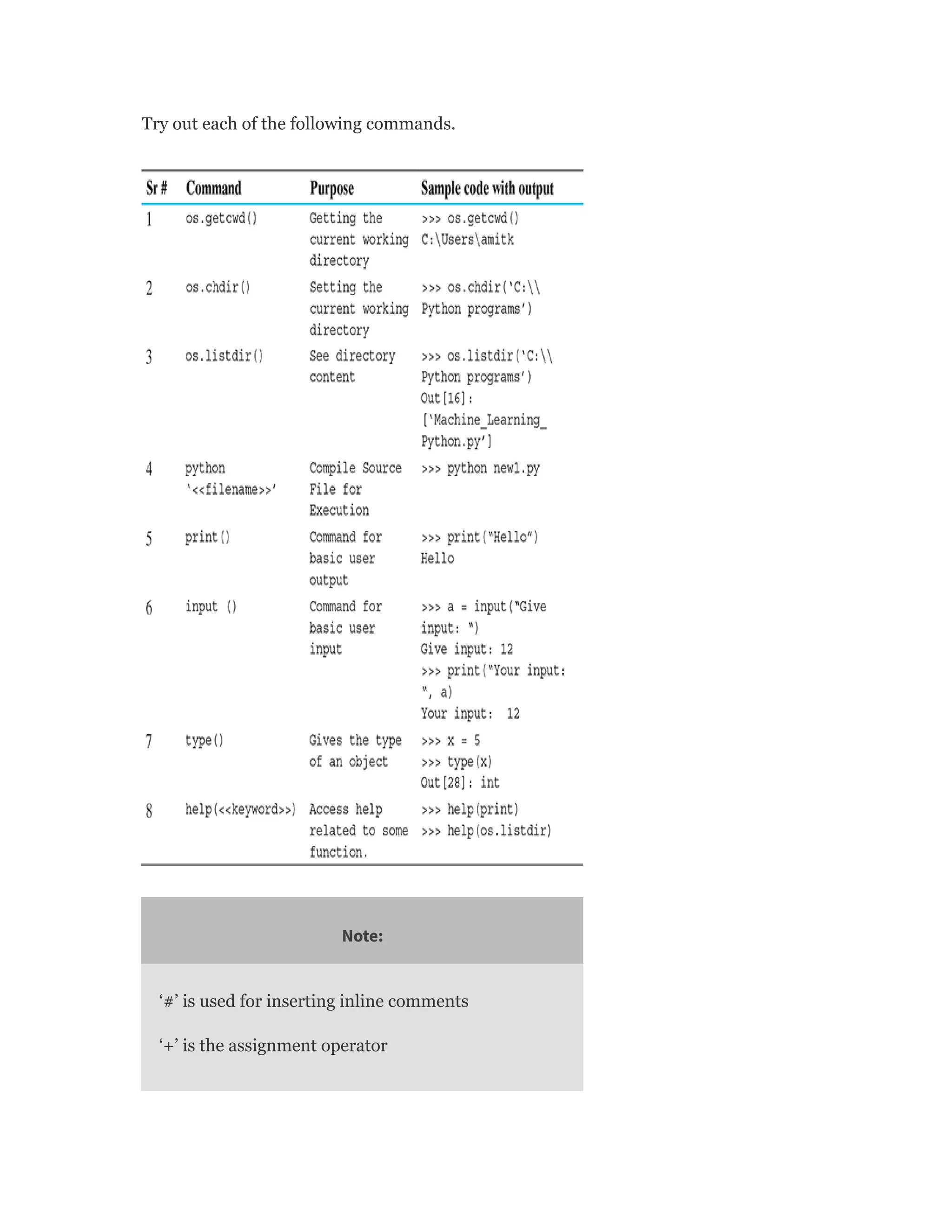
![Note:
“#” is used for inserting inline comments
<- and = are alternative / synonymous assignment
operators
A.1.3.2 Basic data types in R
Vector: This data structure contains similar types of data, i.e.
integer, double, logical, complex, etc. The function c () is used to
create vectors.
> num <- c(1,3.4,-2,-10.85) #numeric vector
> char <- c(“a”,“hello”,“280”) #character vector
> bool <- c(TRUE,FALSE,TRUE,FALSE,FALSE) #logical
vector
> print(num)
[1] 1.0 3.4 -2.0 -10.85
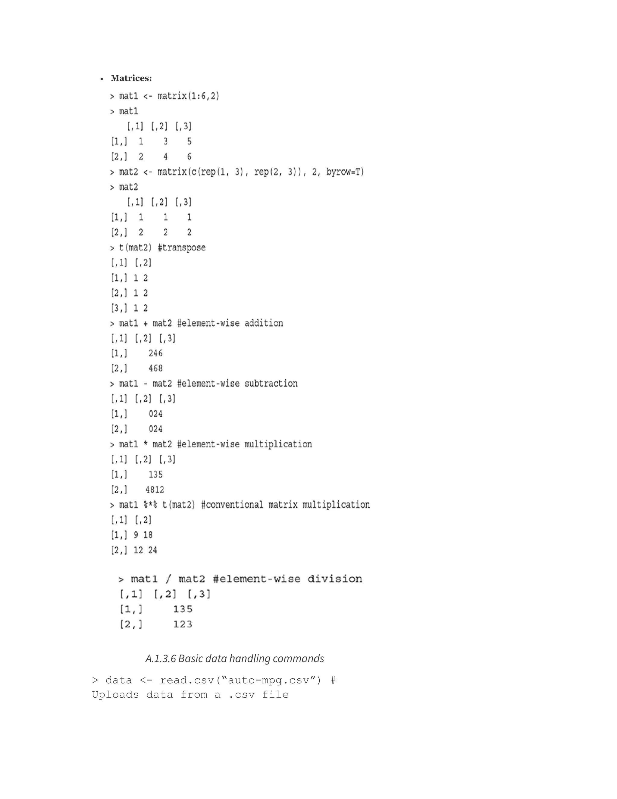
Matrix: Matrix is a 2-D data structure and can be created using the
matrix () function. The values for rows and columns can be defined
using ‘nrow’ and ‘ncol’ arguments. However, providing both is not
required as the other dimension is automatically acquired with the](https://image.slidesharecdn.com/mlsaikatdutt-221115120700-3df1a1af/75/ML_saikat-dutt-pdf-451-2048.jpg)
![help of the length parameter (first index : last index).
List: This data structure is slightly different from vectors in the
sense that it contains a mixture of different data types A list is
created using the list () function.
Factor: The factor stores the nominal values as a vector of integers
in the range [1…k] (where k is the number of unique values in the
nominal variable) and an internal vector of character strings (the
original values) mapped to these items.
> data <- c(‘A’,‘B’,‘B’,‘C’,‘A’,‘B’,‘C’,‘C’,‘B’)
> fact <- factor(data)
> fact
[1] A B B C A B C C B
Levels: A B C
> table(fact) #arranges argument item in a tabular
format fact
A B C #unique items mapped to frequencies
2 4 3
Data frame: This data structure is a special case of list where each
component is of the same length. Data frame is created using the](https://image.slidesharecdn.com/mlsaikatdutt-221115120700-3df1a1af/75/ML_saikat-dutt-pdf-452-2048.jpg)
![frame () function.
A.1.3.3 Loops
For loop
Syntax:
for (variable in sequence)
{
(loop_body)
}
Example: Printing squares of all integers from 1 to 3.
for (i in c(1:3))
{
j = i*i
print(j)
}
[1] 1
[1] 4
[1] 9
While loop
Syntax:
while (condition)](https://image.slidesharecdn.com/mlsaikatdutt-221115120700-3df1a1af/75/ML_saikat-dutt-pdf-453-2048.jpg)
![{
(loop_body)
}
Example: Printing squares of all integers from 1 to 3.
i <- 1
while(i<=3)
{
sqr <- i*i
print(sqr)
i <- i+1
}
[1] 1
[1] 4
[1] 9
If-else statement
Syntax:
if (condition 1)
{
Statement 1
}
else if (condition 2)
{
Statement 2](https://image.slidesharecdn.com/mlsaikatdutt-221115120700-3df1a1af/75/ML_saikat-dutt-pdf-454-2048.jpg)
![}
else
{
Statement 4
}
Example:
x = 0
if (x > 0)
{
print(“positive”)
} else if (x == 0)
{
print(“zero”)
} else
{
print(“negative”)
}
[1] “zero”
A.1.3.4 Writing functions
Writing a function (in a script):
Syntax:
function_name <- function(argument_list)
{](https://image.slidesharecdn.com/mlsaikatdutt-221115120700-3df1a1af/75/ML_saikat-dutt-pdf-455-2048.jpg)
![(function_body)
}
Example: Function to calculate factorial
of an input number n.
factorial <- function (n)
{
fact<-1
for(i in 1:n)
{
fact <-fact*i
}
return(fact)
}
Running the function (after compiling the script by using
source (‘script_name’)):
> f <- factorial(6)
> print(f)
[1] 720
A.1.3.5 Mathematical operations on data types
Vectors:
> n <- 10
> m <- 5
> n + m #addition
[1] 15
> n – m #subtraction
[1] 5
> n * m #multiplication
[1] 50
> n / m #division
[1] 2](https://image.slidesharecdn.com/mlsaikatdutt-221115120700-3df1a1af/75/ML_saikat-dutt-pdf-456-2048.jpg)
![> class(data) # To find the type of the
data set object loaded
[1] “data.frame”
> dim(data) # To find the dimensions, i.e.
the number of rows and columns of the data
set loaded
[1] 398 9
> nrow(data) # To find only the number of
rows
[1] 398
> ncol(data) # To find only the number of
columns
[1] 9
> names (data) #
[1] “mpg” “cylinders” “displacement”
“horsepower” “weight”
[6] “acceleration” “model.year” “origin”
“car.name”
> head (data, 3) # To display the top 3
rows
> tail(data, 3) # To display the bottom 3
rows
> View(data) # To view the data frame
contents in a separate UI
> data[1,9] # Will return cell value of
the 1st row, 9th column of a data frame
[1] chevrolet chevelle malibu
> write.csv(data, “new-auto.csv”) # To
write the contents of a data frame object](https://image.slidesharecdn.com/mlsaikatdutt-221115120700-3df1a1af/75/ML_saikat-dutt-pdf-458-2048.jpg)
![to a .csv file
> rbind(data[1:15,], data[25:35,]) # Bind
sets of rows
> cbind(data[,3], data[,5]) # Bind sets of
columns, with the same number of rows
> data <- data[!data$model.year > 74,]
#Remove all rows with model year greater
than 74
Note:
For advanced data manipulation, the dplyr library
of R (developed by Hadley Wickham et al) can be
leveraged. It is the next version of the plyr package
focused on working with data frames (hence the
name “d”plyr).
A.1.3.7 Advanced data manipulation commands
> library(“dplyr”)
# Functions to project specific columns
> select (data, cylinders) #Selects a
specific feature
> select(data, -cylinders) # De-selects a
specific feature
> select(data,2) #selects columns by
column index
> select(data,2:3) #selects columns by
column index range
> select(data,starts_with(“Cyl”))#Selects
features by pattern match](https://image.slidesharecdn.com/mlsaikatdutt-221115120700-3df1a1af/75/ML_saikat-dutt-pdf-459-2048.jpg)
![unwanted value for an attribute in the data. If there is
such issue, return the rows in which the attribute has
missing/unwanted values. By checking all the attributes,
we find that the attribute ‘horsepower’ has missing
values.
There are six rows in the data set, which have missing
values for the attribute ‘horsepower’. We will have to
remediate these rows before we proceed with the
modelling activities. We will do that shortly.
The easiest and most effective method to detect
outliers is from the box plot of the attributes. In the box
plot, outliers are very clearly highlighted. When we
explore the attributes using box plots in a short while, we
will have a clear view of this aspect.
Let us quickly see the other R commands for obtaining
statistical measures of the numeric attributes.
> range(data$mpg) #Gives minimum and
maximum values
[1] 9.0 46.6](https://image.slidesharecdn.com/mlsaikatdutt-221115120700-3df1a1af/75/ML_saikat-dutt-pdf-465-2048.jpg)
![> diff(range(data$mpg))
[1] 37.6
> quantile(data$mpg)
0% 25% 50% 75% 100%
9.0 17.5 23.0 29.0 46.6
> IQR(data$mpg)
[1] 11.5
> mean(data$mpg)
[1] 23.51457
> median(data$mpg)
[1] 23
> var(data$mpg)
[1] 61.08961
> sd(data$mpg)
[1] 7.815984
Note:
To perform data exploration (as well as data
visualization), the ggplot2 library of R can be
leveraged. Created by Hadley Wickham, the ggplot2
library offers a comprehensive graphics module for
creating elaborate and complex plots.
A.2.2 Basic Plots for Data Exploration
To start using the library functions of ggplot2, we need
to load the library as follows:](https://image.slidesharecdn.com/mlsaikatdutt-221115120700-3df1a1af/75/ML_saikat-dutt-pdf-466-2048.jpg)

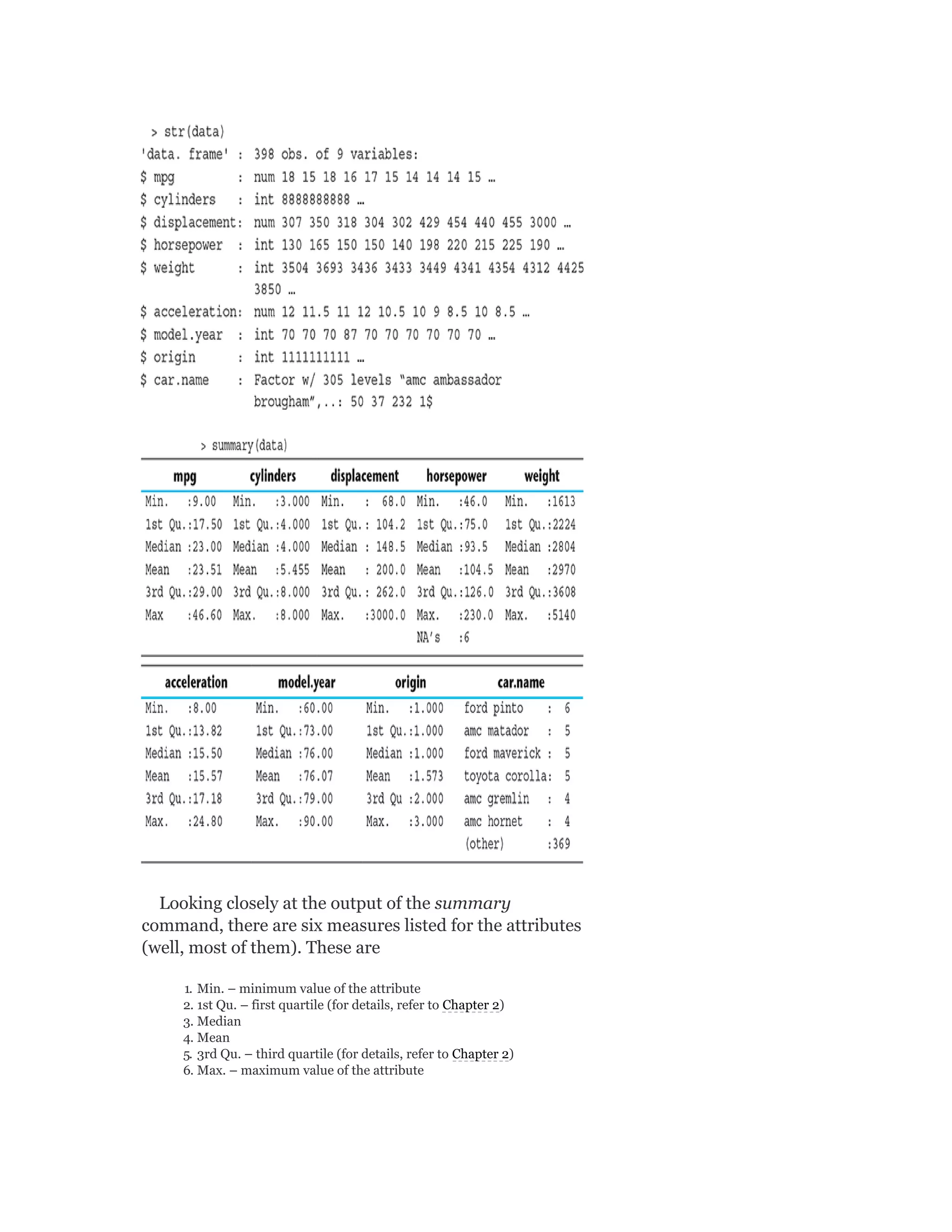
![As we saw in Chapter 2, the primary measures for
remediating outliers and missing values are as follows:
Removing specific rows containing outliers/missing values
Imputing the value (i.e. outlier/missing value) with a standard
statistical measure, e.g. mean or median or mode for that attribute
Estimate the value (i.e. outlier/missing value) on the basis of value of
the attribute in similar records and replace with the estimated value.
Cap the values within 1.5 times IQR limits
Removing outliers/missing values
We have to first identify the outliers. We have already
seen in boxplots that outliers are clearly visible when we
draw the box plot of a specific attribute. Hence, we can
use the same concept as shown in the following code:
> outliers <-
boxplot.stats(data$mpg)$out
Then, those rows can be removed using the code:
> data <- data[!(data$mpg == outliers),]
OR,
> data <- data[-which(data$mpg ==
outliers),]
For missing value identification and removal, the
below code is used:
> data1 <- data[!
(is.na(data$horsepower)),]
Imputing standard values
The code for identification of outliers or missing values
will remain the same. For imputation, depending on
which statistical function is to be used for imputation,
the code will be as follows:
> library(dplyr)
# Only the affected rows are identified
and the value of the attribute is
transformed to the mean value of the
attribute](https://image.slidesharecdn.com/mlsaikatdutt-221115120700-3df1a1af/75/ML_saikat-dutt-pdf-471-2048.jpg)
![> imputedrows <- data[which(data$mpg ==
outliers),] %>% mutate(mpg =
mean(data$mpg))
# Affected rows are removed from the data
set
> outlier_removed_rows <- data[-
which(data$mpg == outliers),]
# Recombine the imputed row and the
remaining part of the data set
> data <- rbind(outlier_removed_rows,
imputedrows)
Almost the same code can be used for imputing
missing values with the only difference being in the
identification of the relevant rows.
> imputedrows <-
data[(is.na(data$horsepower)),]%>% mutate
(horsepower = mean(data$horsepower))
> missval_removed_rows <- data[!
(is.na(data$horsepower)),]
> data <- rbind(outlier_removed_rows,
imputedrows)
Capping of values
The code for identification of outlier values will remain
the same. For capping, generally a value of 1.5 times the
IQR is used for imputation, and the code will be as
follows:
> library(dplyr)
> outliers <- boxplot.stats(data$mpg)$out
> imputedrows <- data[which(data$mpg ==
outliers),] %>% mutate(mpg =
1.5*IQR(data$mpg))](https://image.slidesharecdn.com/mlsaikatdutt-221115120700-3df1a1af/75/ML_saikat-dutt-pdf-472-2048.jpg)
![> outlier_removed_rows <- data[-
which(data$mpg == outliers),]
> data <- rbind(outlier_removed_rows,
imputedrows)
A.3 MODELLING AND EVALUATION
Note:
The caret package (short for Classification And
REgression Training) contains functions to
streamline the model training process for complex
regression and classification problems. The package
contains tools for
data splitting
different pre-processing functionalities
feature selection
model tuning using resampling
model performance evaluation
as well as other functionalities.
A.4 MODEL TRAINING
To start using the functions of the caret package, we
need to include the caret as follows:
> library(caret)
A.4.1 Holdout
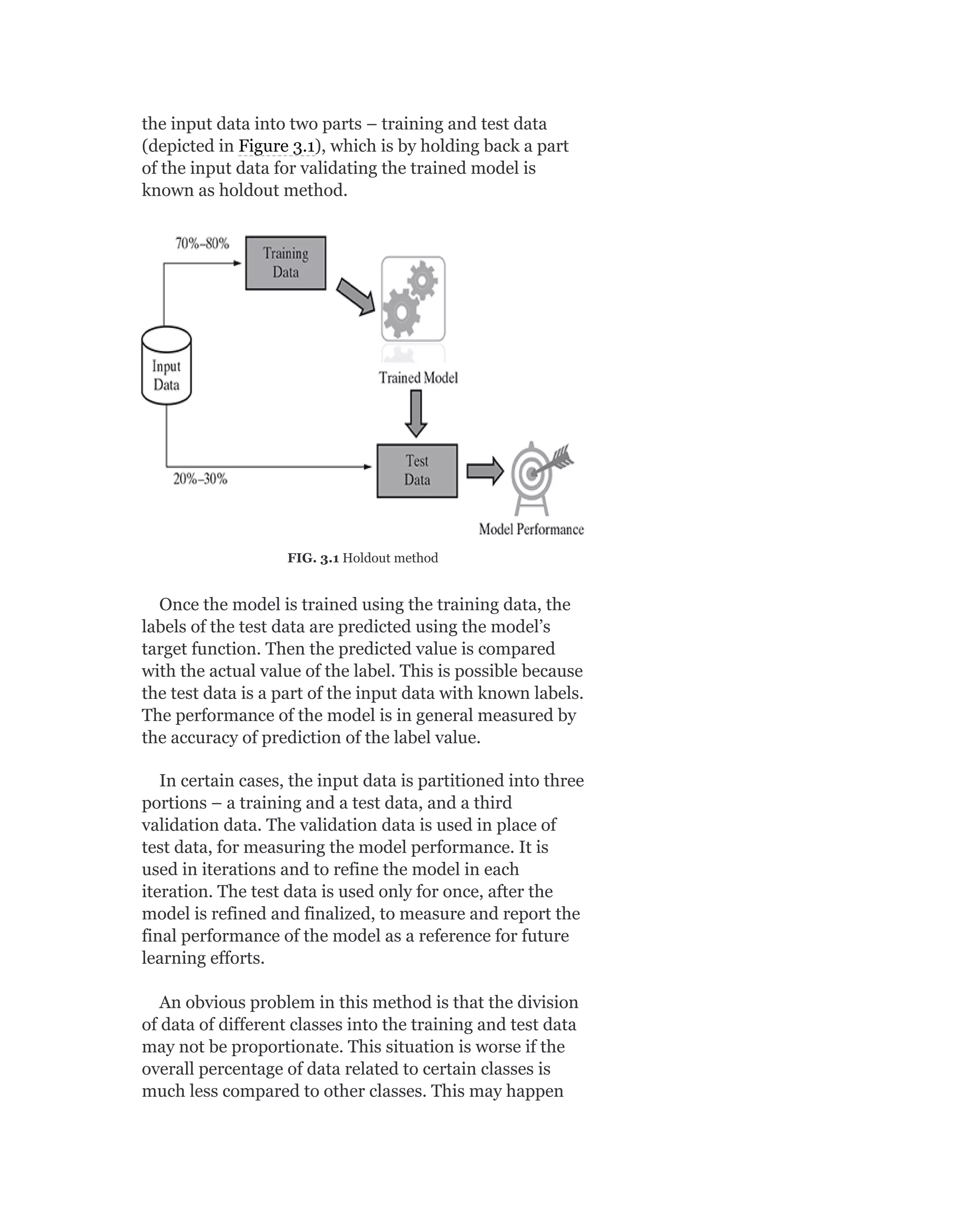
The first step before the start of modelling, in the case of
supervised learning, is to load the input data, holdout a
portion of the input data as test data, and use the
remaining portion as training data for building the
model. Below is the standard procedure to do it.
> inputdata <- read.csv(“btissue.csv”)
> split = 0.7 #Ratio in which the input
data is to be split to training and test
data. A split value = 0.7 indicates 70% of](https://image.slidesharecdn.com/mlsaikatdutt-221115120700-3df1a1af/75/ML_saikat-dutt-pdf-473-2048.jpg)
![the data will be training data, i.e. 30%
of the input data is retained as test data
> set.seed(123) # This step is optional,
needed for result reproducibility
> trainIndex <- createDataPartition (y =
inputdata$class, p = split, list = FALSE)
# Does a stratified random split
of data into training and test sets
> train_ds <- inputdata [trainIndex,]
> test_ds <- inputdata [-trainIndex,]
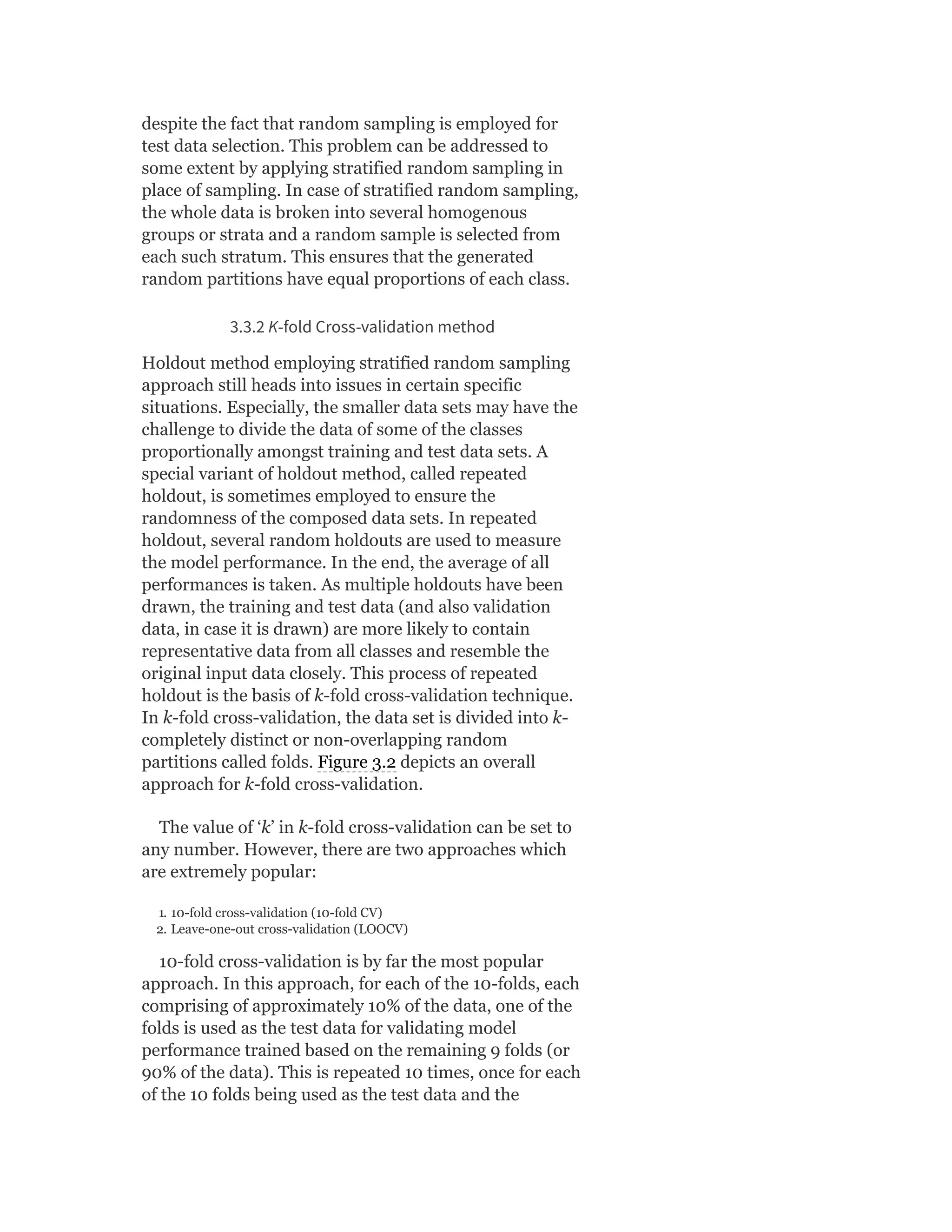
A.4.2 K-Fold Cross-Validation
Let us do a 10-fold cross-validation. For creating the
cross-validation, functions from the caret package can be
used as follows:
Next, we perform the data holdout.
train_ds <- inputdata [-
ten_folds$Fold01,]
test_ds <- inputdata [ten_folds$Fold01,]
Note:](https://image.slidesharecdn.com/mlsaikatdutt-221115120700-3df1a1af/75/ML_saikat-dutt-pdf-474-2048.jpg)


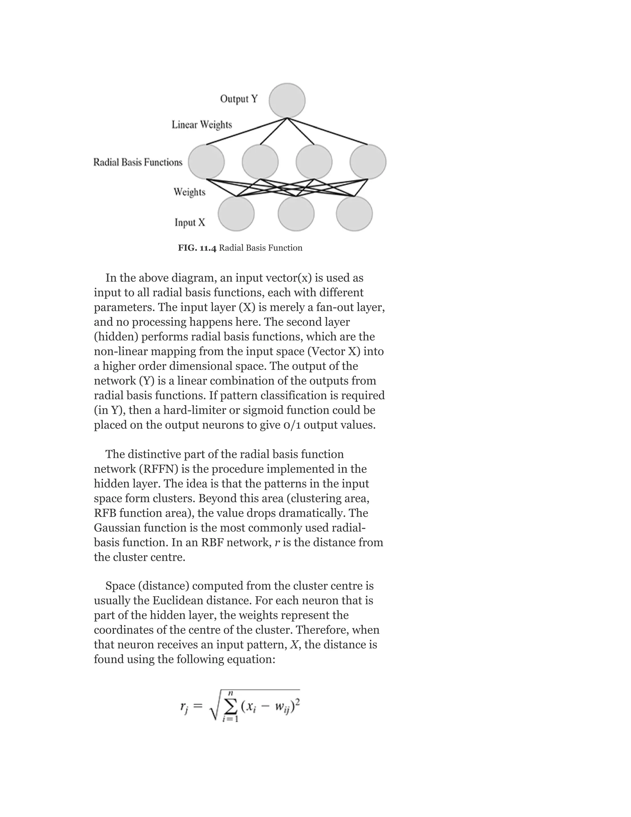
![FIG. A.7 Performance evaluation of a classification model (Decision Tree)
> predictions <- predict(model, test_ds,
na.action = na.pass)
> cm <- confusionMatrix(predictions,
test_ds$class)
> print(cm)
> print(cm$overall[‘Accuracy’])
A.4.5.2 Supervised learning - regression
The summary function, when applied to a regression
model, displays the different performance measures such
as residual standard error, multiple R-squared, etc., both
for simple and multiple linear regression.](https://image.slidesharecdn.com/mlsaikatdutt-221115120700-3df1a1af/75/ML_saikat-dutt-pdf-477-2048.jpg)
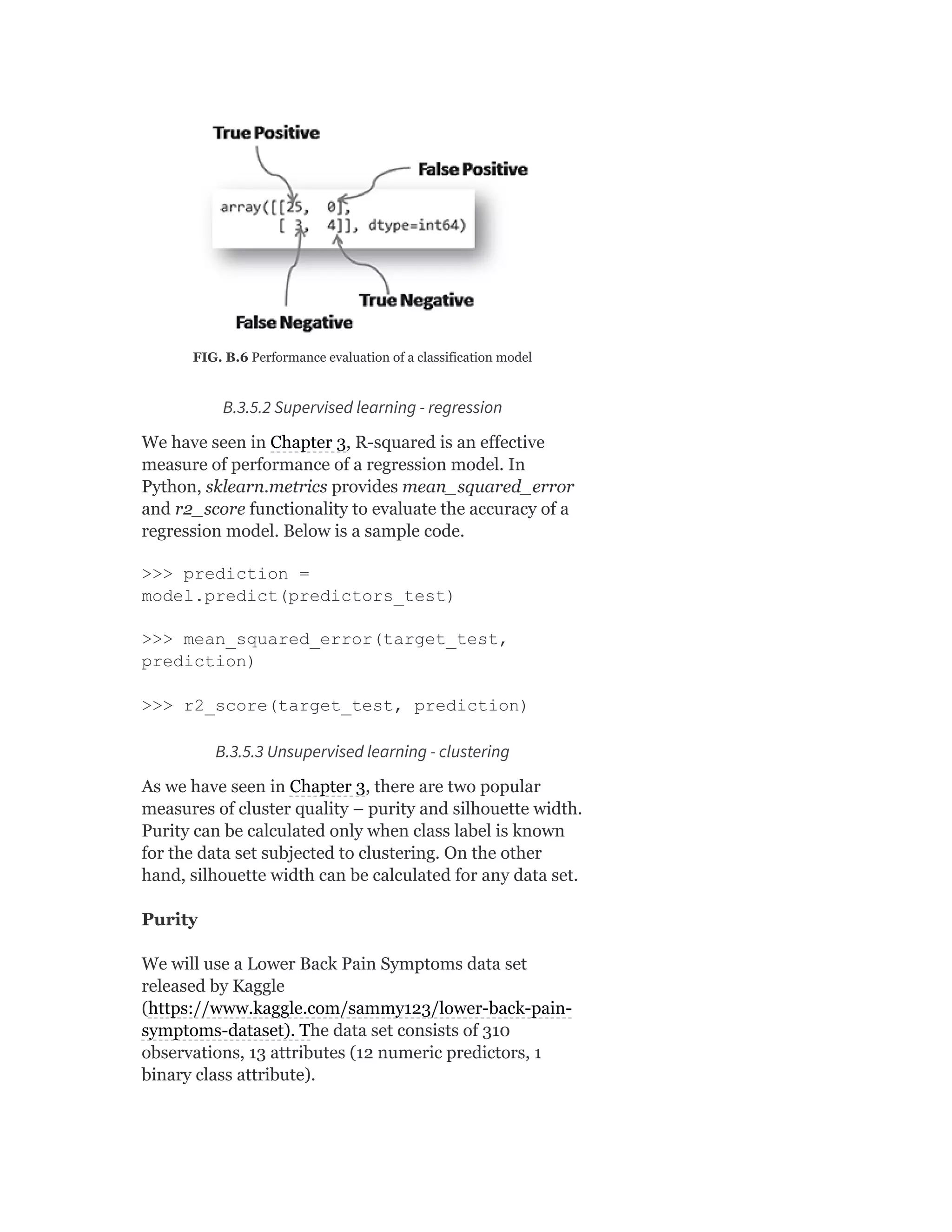
![A.4.5.3 Unsupervised learning - clustering
As we have seen in Chapter 3, there are two popular
measures of cluster quality: purity and silhouette width.
Purity can be calculated only when class label is known
for the data set subjected to clustering. On the other
hand, silhouette width can be calculated for any data set.
Purity
We will use a Lower Back Pain Symptoms data set
released by Kaggle
(https://www.kaggle.com/sammy123/lower-back-pain-
symptoms-dataset). The data set spine.csv consists of
310 observations and 13 attributes (12 numeric
predictors, 1 binary class attribute).
> library(fpc)
> data <- read.csv(“spine.csv”) #Loading
the Kaggle data set
> data_wo_class <- data[,-length(data)]
#Stripping off the class attribute from
the data set before clustering
> class <- data[,length(data)] #Storing
the class attribute in a separate variable
for later use
> dis = dist(data_wo_class)^2
> res = kmeans(data_wo_class,2) #Can use
other clustering algorithms too
#Let us define a custom function to
compare cluster value with the original
class value and calculate the percentage
match
ClusterPurity <- function(clusters,
classes) {
sum(apply(table(classes, clusters), 2,
max)) / length(clusters)](https://image.slidesharecdn.com/mlsaikatdutt-221115120700-3df1a1af/75/ML_saikat-dutt-pdf-479-2048.jpg)
![}
> ClusterPurity(res$cluster, class)
Output
[1] 0.6774194
Silhouette width
Use the R library cluster to find out/plot the silhouette
width of the clusters formed. The piece of code below
clusters the records in the data set spinem.csv (the same
data set as spine.csv with the target variable removed)
using the k-means algorithm and then calculates the
silhouette width of the clusters formed.
> library (cluster)
> data <- read.csv(“spinem.csv”)
> dis = dist(data)^2
> res = kmeans(data,2) #Can use other
clustering algorithms too
> sil_width <- silhouette (res$cluster,
dis)
> sil_summ <- summary(sil_width)
> sil_summ$clus.avg.widths # Returns
silhouette width of each cluster
> sil_summ$avg.width # Returns silhouette
width of the overall data set
Output
Silhouette width of each cluster:
1 2
0.7473583 0.1921082
Silhouette width of the overall data set:](https://image.slidesharecdn.com/mlsaikatdutt-221115120700-3df1a1af/75/ML_saikat-dutt-pdf-480-2048.jpg)
![[1] 0.5413785
A.5 FEATURE ENGINEERING
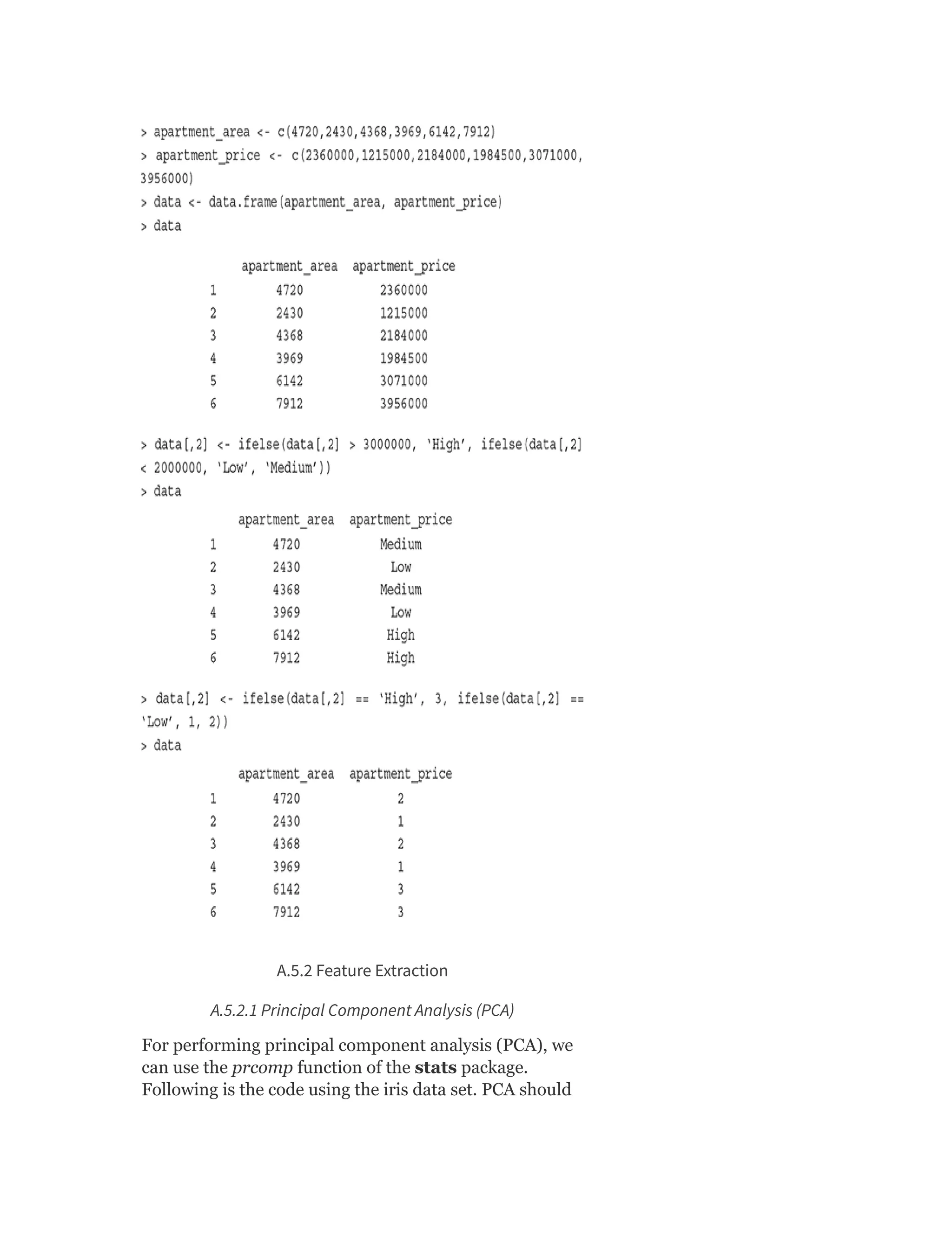
A.5.1 Feature Construction
For performing feature construction, we can use mutate
function of the dplyr package. Following is a small code
for feature construction using the iris data set.
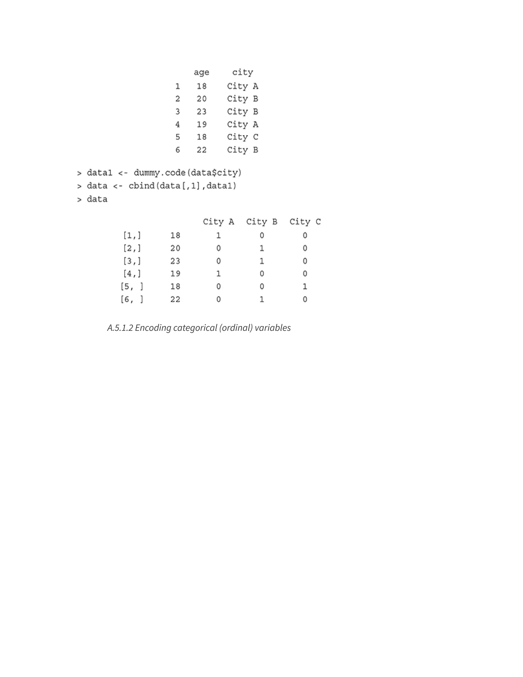
A.5.1.1 Dummy coding categorical (nominal) variables
As in the above case, we can use the dummy.code
function of the psych package to encode categorical
variables. Following is a small code for the same.
> library(psych)
> age <- c(18,20,23,19,18,22)
> city <- c(‘City A’,‘City B’,‘City
A’,‘City C’,‘City B’)
> data <- data.frame(age, city)
> data](https://image.slidesharecdn.com/mlsaikatdutt-221115120700-3df1a1af/75/ML_saikat-dutt-pdf-481-2048.jpg)
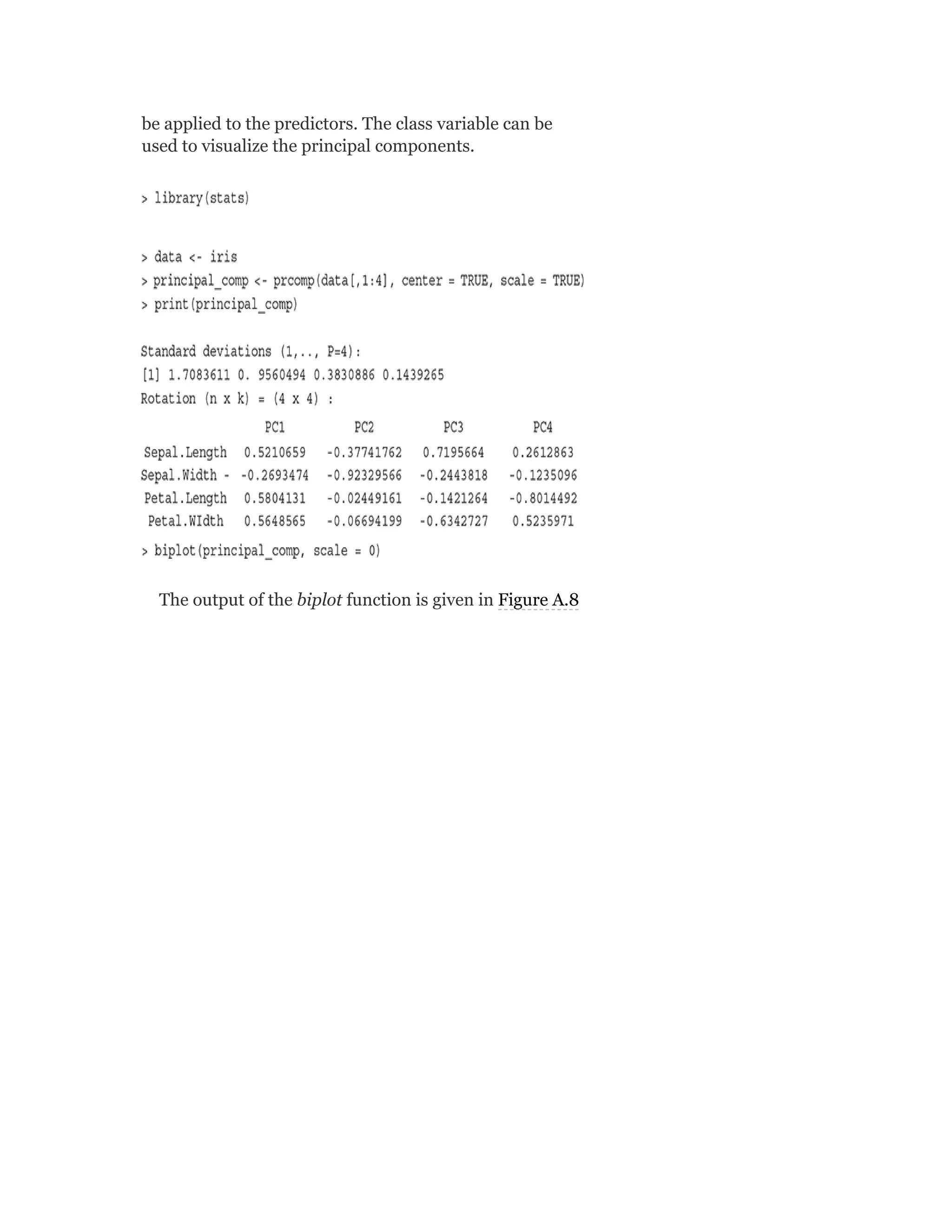
![FIG. A.8 Principal components of the iris data set
A.5.2.2 Singular Value Decomposition (SVD)
For performing singular value decomposition, we can use
the svd function of the stats package. Following is the
code using the iris data set.
> sing_val_decomp <- svd(iris[,1:4])
> print(sing_val_decomp$d)
Output:
[1] 95.959914 17.761034 3.460931 1.884826
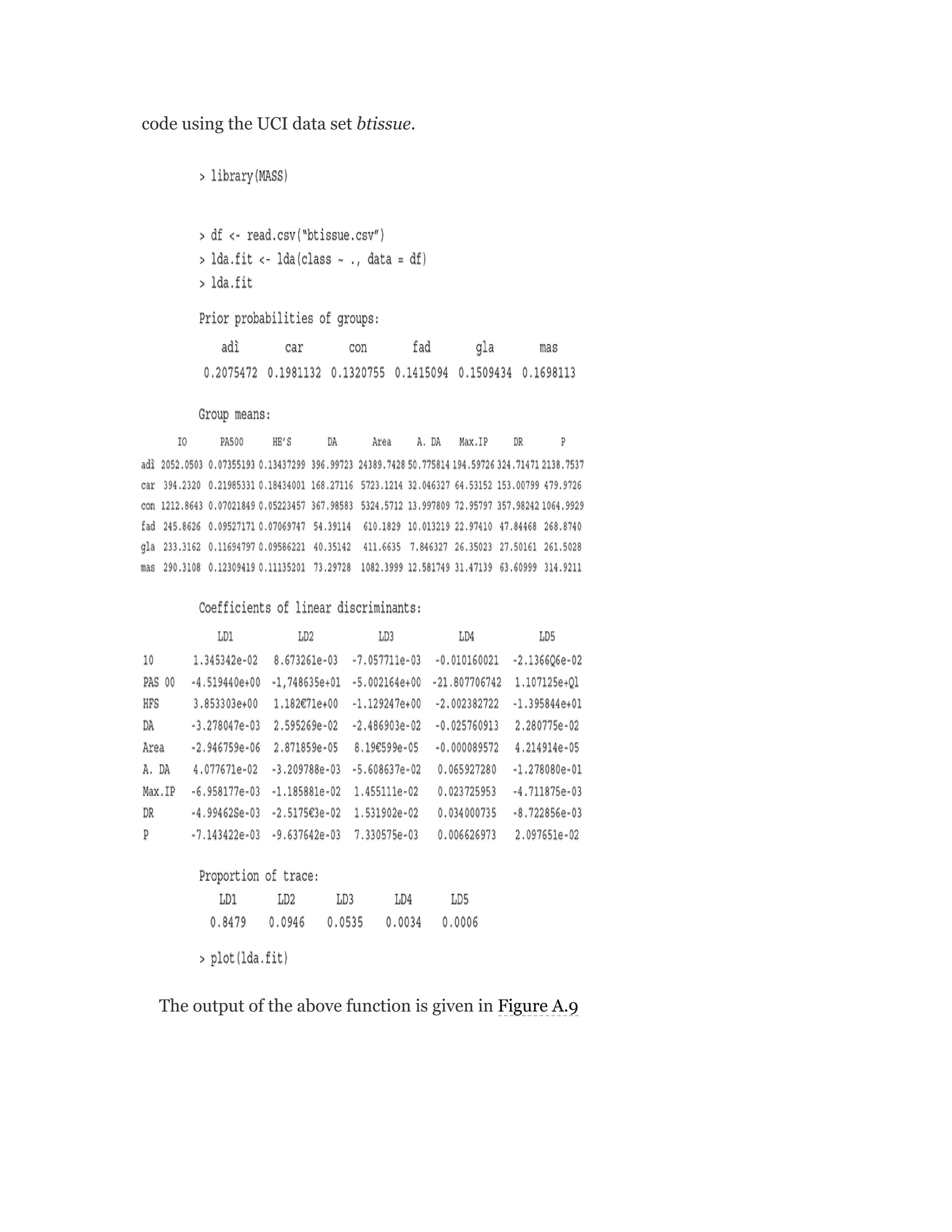
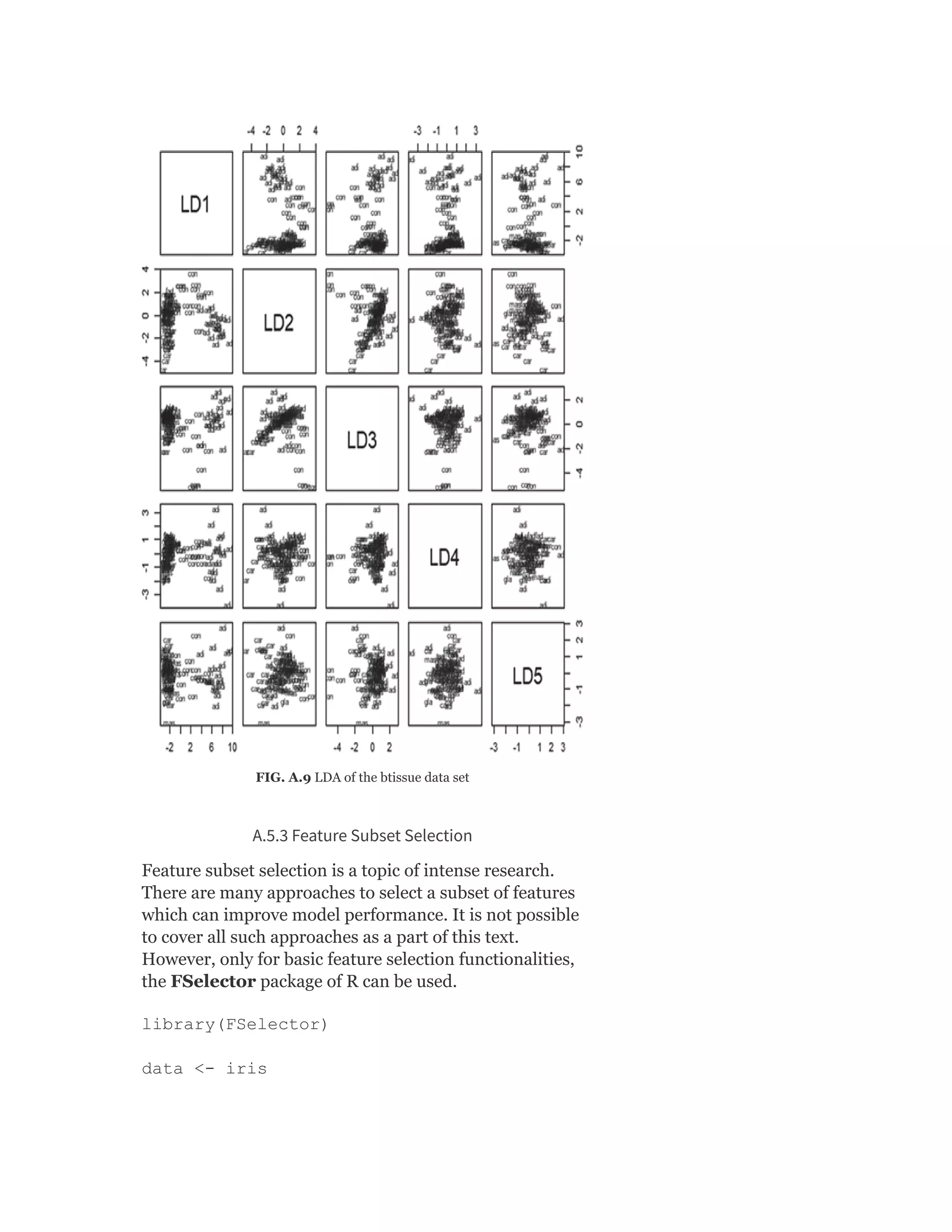
A.5.2.3 Linear Discriminant Analysis (LDA)
For performing linear discriminant analysis, we can use
the lda function of the MASS package. Following is the](https://image.slidesharecdn.com/mlsaikatdutt-221115120700-3df1a1af/75/ML_saikat-dutt-pdf-486-2048.jpg)
![feat_subset <- cfs(Species ~ ., data) #
Selects feature subset using correlation
and entropy measures for continuous and
discrete data
Below is a programme to perform feature subset
selection before applying the same for training a model.
library(caret)
library(FSelector)
inputdata <- read.csv(“apndcts.csv”)
split = 0.7
set.seed(123)
trainIndex <- createDataPartition (y =
inputdata$class, p = split, list = FALSE)
train_ds <- inputdata [trainIndex,]
test_ds <- inputdata [-trainIndex,]
feat_subset <- cfs(class ~ ., train_ds)
#Feature selection done class <-
train_ds$class
train_ds <- cbind(train_ds[feat_subset],
class) # Subset training data created
class <- test_ds$class
test_ds <- cbind(test_ds[feat_subset],
class) # Subset test data created
train_ds$class <-
as.factor(train_ds$class)
test_ds$class <- as.factor(test_ds$class)
# Applying Decision Tree classifier
here. Any other model can also be applied
…](https://image.slidesharecdn.com/mlsaikatdutt-221115120700-3df1a1af/75/ML_saikat-dutt-pdf-489-2048.jpg)
![model <- train(class ~ ., method =
“rpart”, data = train_ds) predictions <-
predict(model, test_ds, na.action =
na.pass)
cm <- confusionMatrix(predictions,
test_ds$class)
cm$overall[‘Accuracy’]
Note:
The e1071 package is an important R package which
contains many statistical functions along with some
critical classification algorithms such as Naïve Bayes
and support vector machine (SVM). It is created by
David Meyer and team and maintained by David
Meyer.
A.6 MACHINE LEARNING MODELS
A.6.1 Supervised Learning – Classification
In Chapters 6, 7, and 8, conceptual overview of different
supervised learning algorithms has been presented. Now,
you will understand how to implement them using R. For
the sake of simplicity, the code for implementing each of
the algorithms is kept as consistent as possible. Also, we
have used benchmark data sets from UCI repository
(these data sets will also be available online, refer to the
URL https://archive.ics.uci.edu/ml).
A.6.1.1 Naïve Bayes classifier
To implement this classifier, the naiveBayes function of
the e1071 package has been used. The full code for the
implementation is given below.
> library(caret)
> library (e1071)](https://image.slidesharecdn.com/mlsaikatdutt-221115120700-3df1a1af/75/ML_saikat-dutt-pdf-490-2048.jpg)
![> inputdata <- read.csv(“apndcts.csv”)
> split = 0.7
> set.seed(123)
> trainIndex <- createDataPartition (y =
inputdata$class, p = split, list = FALSE)
> train_ds <- inputdata [trainIndex,]
> test_ds <- inputdata [-trainIndex,]
> train_ds$class <-
as.factor(train_ds$class) #Pre-processing
step
> test_ds$class <-
as.factor(test_ds$class) #Pre-processing
step
> model <- naiveBayes (class ~ ., data =
train_ds)
> predictions <- predict(model, test_ds,
na.action = na.pass)
> cm <- confusionMatrix(predictions,
test_ds $class)
> cm$overall[‘Accuracy’]
Output Accuracy:
0.8387097
A.6.1.2 kNN classifier
To implement this classifier, the knn function of the
class package has been used. The full code for the
implementation is given below.
> library(caret)
> library (class)](https://image.slidesharecdn.com/mlsaikatdutt-221115120700-3df1a1af/75/ML_saikat-dutt-pdf-491-2048.jpg)
![> inputdata <- read.csv(“apndcts.csv”)
> split = 0.7
> set.seed(123)
> trainIndex <- createDataPartition (y =
inputdata$class, p = split, list = FALSE)
> train_ds <- inputdata [trainIndex,]
> test_ds <- inputdata [-trainIndex,]
> train_ds$class <-
as.factor(train_ds$class) #Pre-processing
step
> test_ds$class <-
as.factor(test_ds$class) #Pre-processing
step
> model <- knn(train_ds, test_ds,
train_ds$class, k = 3)
> cm <- confusionMatrix(model,
test_ds$class)
> cm$overall[‘Accuracy’]
Output Accuracy:
1
A.6.1.3 Decision tree classifier
To implement this classifier implementation, the train
function of the caret package can be used with a
parameter method = “rpart” to indicate that the train
function will use the decision tree classifier. Optionally,
the rpart function of the rpart package can also be used.
The full code for the implementation is given below.
> library(caret)
> library(rpart) # Optional](https://image.slidesharecdn.com/mlsaikatdutt-221115120700-3df1a1af/75/ML_saikat-dutt-pdf-492-2048.jpg)
![> inputdata <- read.csv(“apndcts.csv”)
> split = 0.7
> set.seed(123)
> trainIndex <- createDataPartition (y =
inputdata$class, p = split, list = FALSE)
> train_ds <- inputdata [trainIndex,]
> test_ds <- inputdata [-trainIndex,]
> train_ds$class <-
as.factor(train_ds$class) #Pre-processing
step
> test_ds$class <-
as.factor(test_ds$class) #Pre-processing
step
> model <- train(class ~ ., method =
“rpart”, data = train_ds, prox = TRUE)
# May also use the rpart function as shown
below …
#> model <- rpart(formula = class ~ .,
data = train_ds) # Optional
> predictions <- predict(model, test_ds,
na.action = na.pass)
> cm <- confusionMatrix(predictions,
test_ds $class)
> cm$overall[‘Accuracy’]
Output Accuracy:
0.8387097
A.6.1.4 Random forest classifier
To implement this classifier, the train function of the
caret package can be used with the parameter method =](https://image.slidesharecdn.com/mlsaikatdutt-221115120700-3df1a1af/75/ML_saikat-dutt-pdf-493-2048.jpg)
![“rf” to indicate that the train function will use the
decision tree classifier. Optionally, the randomForest
function of the randomForest package can also be
used. The full code for the implementation is given
below.
> library(caret)
> library(randomForest) # Optional
> inputdata <- read.csv(“apndcts.csv”)
> split = 0.7
> set.seed(123)
> trainIndex <- createDataPartition (y =
inputdata$class, p = split, list = FALSE)
> train_ds <- inputdata [trainIndex,]
> test_ds <- inputdata [-trainIndex,]
> train_ds$class <-
as.factor(train_ds$class) #Pre-processing
step
> test_ds$class <-
as.factor(test_ds$class) #Pre-processing
step
> model <- train(class ~ ., method = “rf”,
data = train_ds, prox = TRUE)
# May also use the randomForest function
as shown below …
#> model <- randomForest(class ~ . , data
= train_ds, ntree=400)
> predictions <- predict(model, test_ds,
na.action = na.pass)
> cm <- confusionMatrix(predictions,
test_ds $class)](https://image.slidesharecdn.com/mlsaikatdutt-221115120700-3df1a1af/75/ML_saikat-dutt-pdf-494-2048.jpg)
![> cm$overall[‘Accuracy’]
Output Accuracy:
0.8387097
A.6.1.5 SVM classifier
To implement this classifier, the svm function of the
e1071 package has been used. The full code for the
implementation is given below.
> library(caret)
> library (e1071)
> inputdata <- read.csv(“apndcts.csv”)
> split = 0.7
> set.seed(123)
> trainIndex <- createDataPartition (y =
inputdata$class, p = split, list = FALSE)
> train_ds <- inputdata [trainIndex,]
> test_ds <- inputdata [-trainIndex,]
> train_ds$class <-
as.factor(train_ds$class) #Pre-processing
step
> test_ds$class <-
as.factor(test_ds$class) #Pre-processing
step
> model <- svm(class ~ ., data = train_ds)
> predictions <- predict(model, test_ds,
na.action = na.pass)
> cm <- confusionMatrix(predictions,
test_ds $class)
> cm$overall[‘Accuracy’]](https://image.slidesharecdn.com/mlsaikatdutt-221115120700-3df1a1af/75/ML_saikat-dutt-pdf-495-2048.jpg)
![Output Accuracy:
0.8709677
A.6.2 Supervised Learning – Regression
As discussed in Chapter 9, two main algorithms used for
regression are simple linear regression and multiple
linear regression. Implementation of both the algorithms
in R code is shown below.
> data <- read.csv(“auto-mpg.csv”)
> attach(data) # Data set is attached to
the R search path, which means that while
evaluating a variable, objects in the data
set can be accessed by simply giving their
names. So, instead of “data$mpg”, simply
giving “mpg” will suffice.
> data <-
data[!is.na(as.numeric(as.character(horsep
ower))),]
> data <- mutate(data, horsepower =
as.numeric(horsepower))
> outliers_mpg <- boxplot.stats(mpg)$out
> data <- data[-which(mpg ==
outliers_mpg),]
> outliers_cylinders <-
boxplot.stats(cylinders)$out
> data <- data[-which(cylinders ==
outliers_cylinders),]
> outliers_displacement <-
boxplot.stats(displacement)$out
> data <- data[-which(displacement ==
outliers_displacement),]](https://image.slidesharecdn.com/mlsaikatdutt-221115120700-3df1a1af/75/ML_saikat-dutt-pdf-496-2048.jpg)
![> outliers_weight <-
boxplot.stats(weight)$out
> data <- data[-which(weight ==
outliers_weight),]
> outliers_acceleration <-
boxplot.stats(acceleration)$out
> data <- data[-which(acceleration ==
outliers_acceleration),]
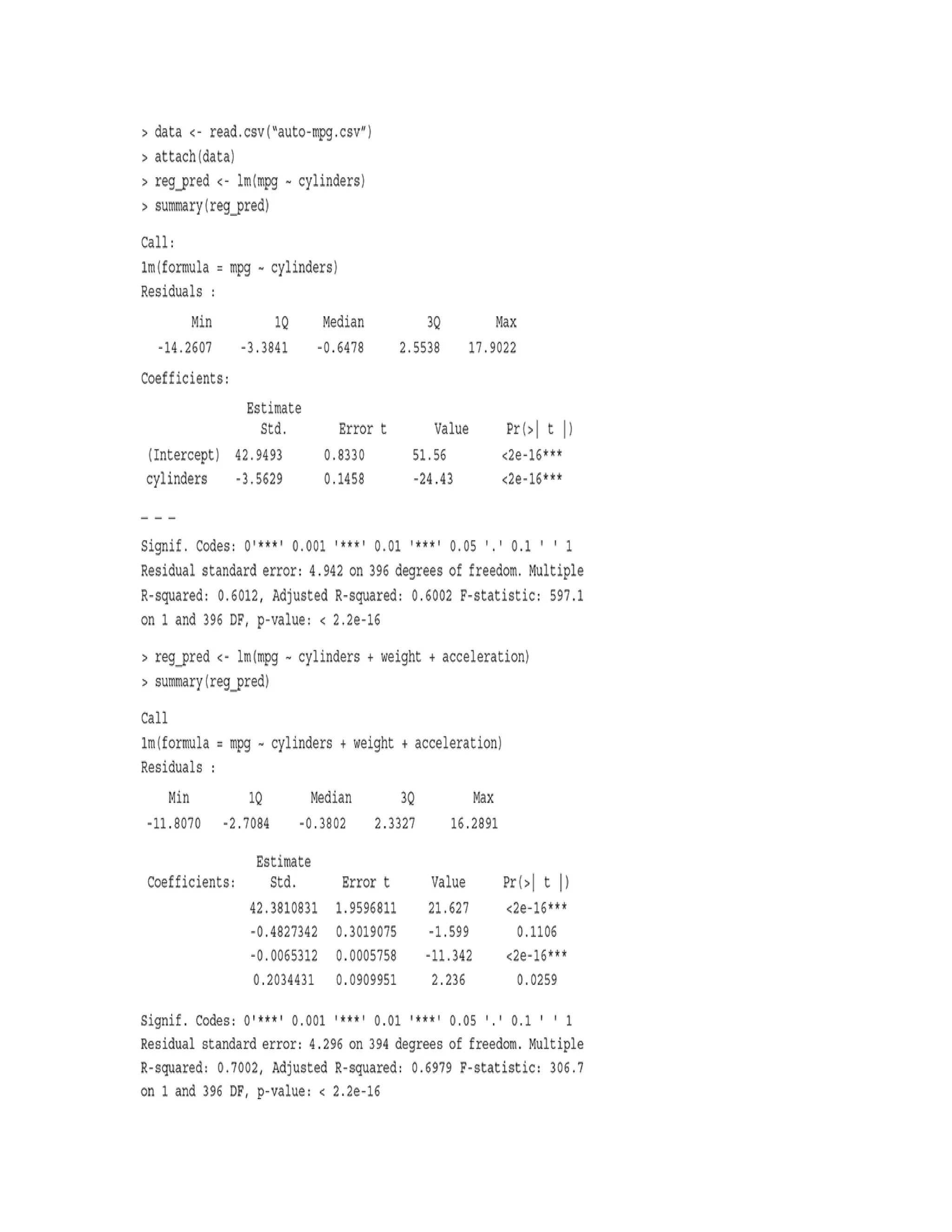
A.6.2.1 Simple linear regression
> reg_pred <- lm(mpg ~ cylinders)
> summary(reg_pred)
A.6.2.2 Multiple linear regression
> reg_pred <- lm(mpg ~ cylinders +
displacement)
> reg_pred <- lm(mpg ~ cylinders + weight
+ acceleration)
> reg_pred <- lm(mpg ~ cylinders +
displacement + horsepower + weight +
acceleration)
A.6.3 Unsupervised Learning
To implement the k-means algorithm, the k-means
function of the cluster package has been used. Also,
because silhouette width is a more generic performance
measure, it has been used here. The complete R code for
the implementation is given below.
> library (cluster)
> data <- read.csv(“spinem.csv”)
> dis = dist(data)^2
> res = kmeans(data,2)](https://image.slidesharecdn.com/mlsaikatdutt-221115120700-3df1a1af/75/ML_saikat-dutt-pdf-497-2048.jpg)
![> sil_width <- silhouette (res$cluster,
dis)
> sil_summ <- summary(sil_width)
> sil_summ$avg.width # Returns silhouette
width of the overall data set
Output Accuracy:
[1] 0.5508955
A.6.4 Neural Network
To implement this classifier, the neuralnet function of
the neuralnet package has been used. The full code for
the implementation is given below.
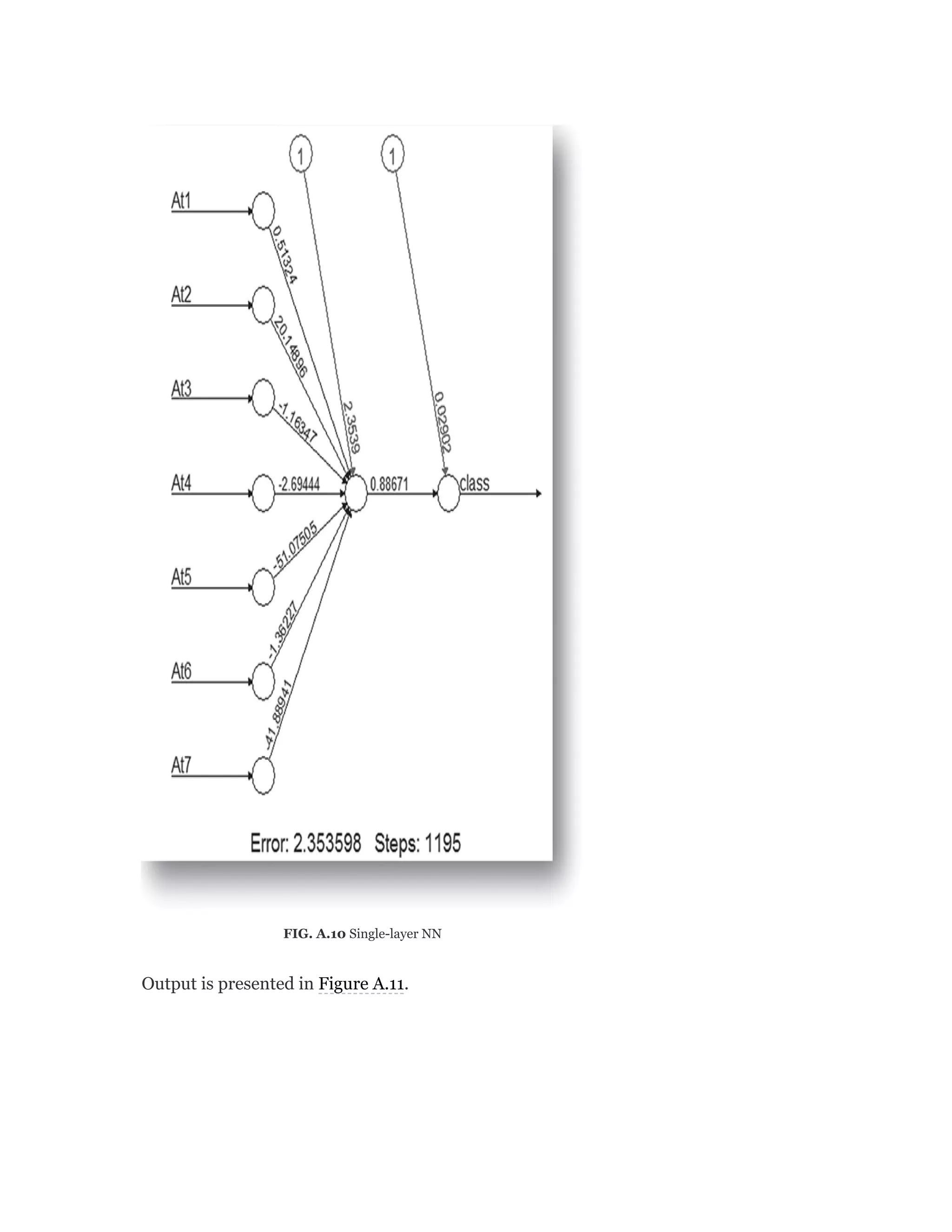
A.6.4.1 Single-layer feedforward neural network
> library(caret)
> library(neuralnet)
> inputdata <- read.csv(“apndcts.csv”)
> split = 0.7
> set.seed(123)
> trainIndex <- createDataPartition (y =
inputdata$class, p = split, list = FALSE)
> train_ds <- inputdata [trainIndex,]
> test_ds <- inputdata [-trainIndex,]
> model <- neuralnet(class ~ At1 + At2 +
At3 + At4 + At5 + At6 + At7, train_ds)
> plot(model)
Output is presented in Figure A.10.
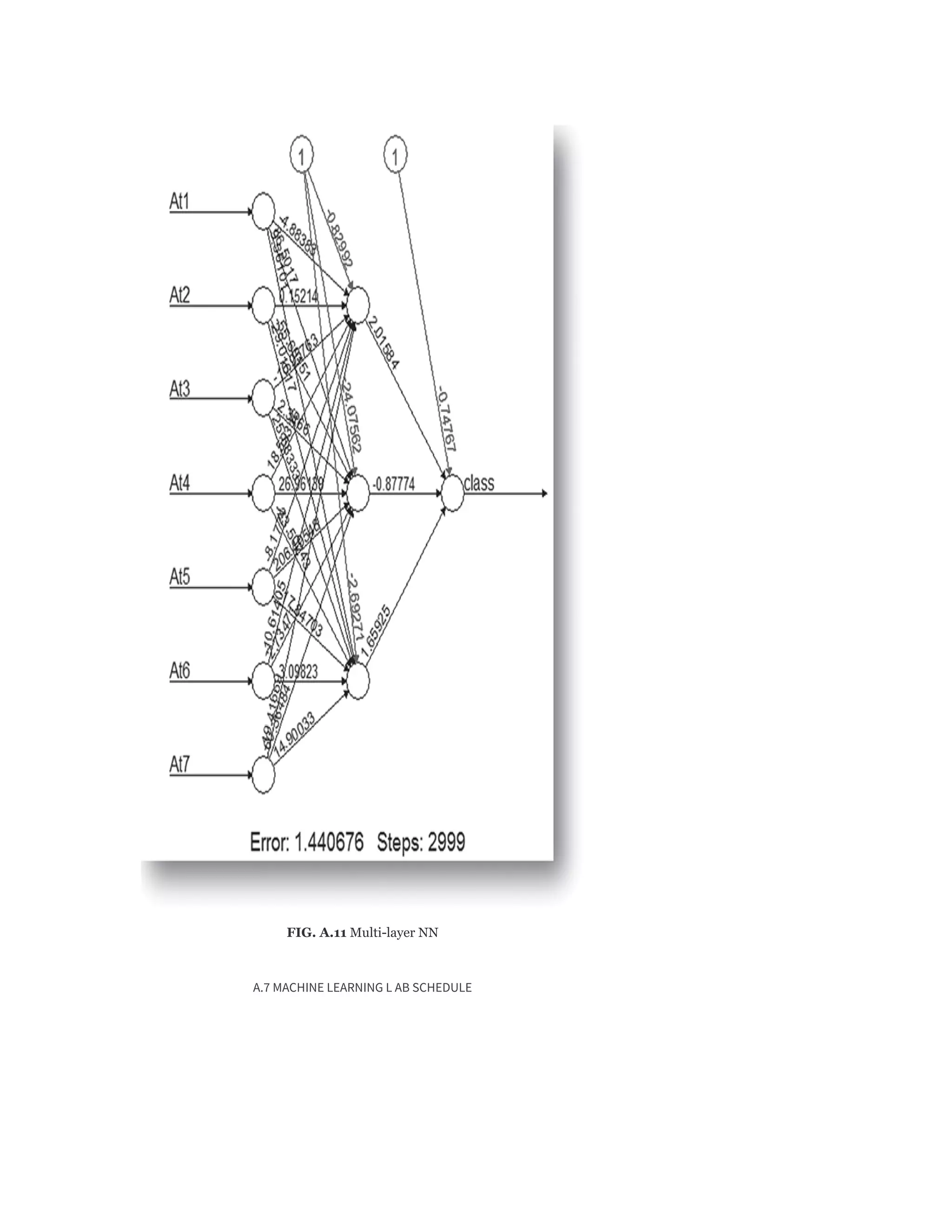
A.6.4.2 Multi-layer feedforward neural network](https://image.slidesharecdn.com/mlsaikatdutt-221115120700-3df1a1af/75/ML_saikat-dutt-pdf-498-2048.jpg)
![> library(caret)
> library(neuralnet)
> inputdata <- read.csv(“apndcts.csv”)
> split = 0.7 > set.seed(123)
> trainIndex <- createDataPartition (y =
inputdata$class, p = split, list = FALSE)
> train_ds <- inputdata [trainIndex,]
> test_ds <- inputdata [-trainIndex,]
> model <- neuralnet(class ~ At1 + At2 +
At3 + At4 + At5 + At6 + At7, train_ds,
hidden = 3) # Multi-layer NN
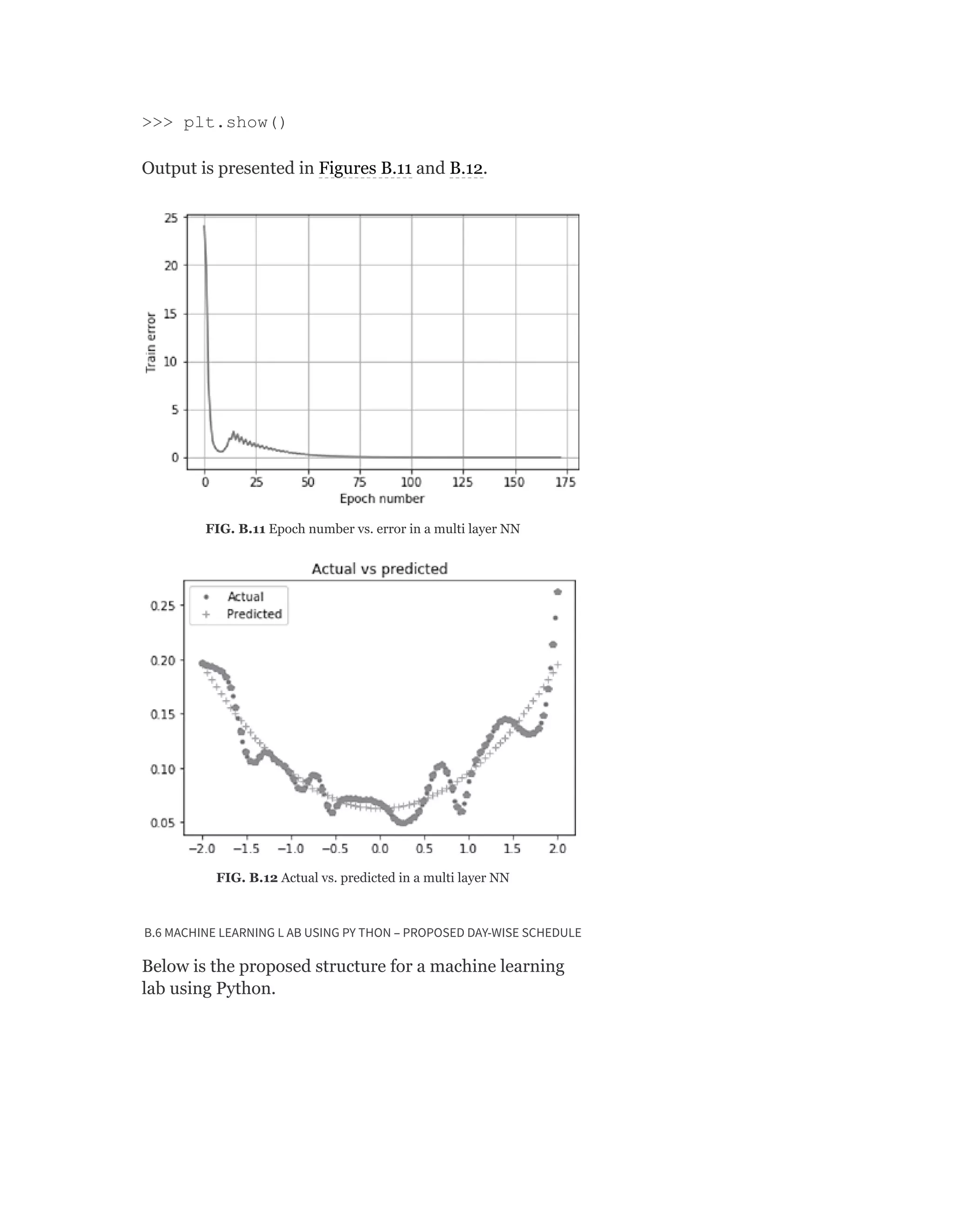
> plot(model)](https://image.slidesharecdn.com/mlsaikatdutt-221115120700-3df1a1af/75/ML_saikat-dutt-pdf-499-2048.jpg)


![B.1.3.2 Basic data types in Python
Python has five standard data types −
1. Number
2. String
3. List
4. Tuple
5. Dictionary
Though Python has all the basic data types, Python
variables do not need explicit declaration to reserve
memory space. The declaration happens automatically
when you assign a value to a variable. The equal sign (=)
is used to assign values to variables.
The operand to the left of the = operator is the name of
the variable and the operand to the right of the =
operator is the value stored in the variable. For example
−
>>> var1 = 4
>>> var2 = 8.83
>>> var3 = “Machine Learning”
>>> type(var1)
Out[38]: int
>>> print(var1)
4
>>> type(var2)
Out[39]: float
>>> print(var2)
8.83
>>> type(var3)
Out[40]: str](https://image.slidesharecdn.com/mlsaikatdutt-221115120700-3df1a1af/75/ML_saikat-dutt-pdf-509-2048.jpg)
![>>> print(var3)
Machine Learning
Python variables can be easily typecasted from one
data type to another by using its datatype name as a
function (actually a wrapper class) and passing the
variable to be typecasted as a parameter. But not all data
types can be transformed into another like String to
integer/number is impossible (that’s obvious!).
>>> var2 = int(var2)
>>> print (var2)
8
>>> type (var2)
Out[42]: int
B.1.3.3 for–while Loops & if–else Statement
For loop
Syntax:
for i in range(<lowerbound>,<upperbound>,
<interval>):
print(i*i)
Example: Printing squares of all integers from 1 to 3.
for i in range(1,4):
print(i*i)
1
4
9
for i in range(0,4,2):](https://image.slidesharecdn.com/mlsaikatdutt-221115120700-3df1a1af/75/ML_saikat-dutt-pdf-510-2048.jpg)


![>>> n + m #addition
Out[53]: 15
>>> n - m #subtraction
Out[55]: 5
>>> n * m #multiplication
Out[56]: 50
>>> n / m #division
Out[57]: 2.0
Matrices:](https://image.slidesharecdn.com/mlsaikatdutt-221115120700-3df1a1af/75/ML_saikat-dutt-pdf-513-2048.jpg)

![B.1.3.6 Basic data handling commands
>>> import pandas as pd # “pd” is just
an alias for pandas
>>> data = pd.read_csv(“auto-mpg.csv”) #
Uploads data from a .csv file
>>> type(data) # To find the type of
the data set object loaded
pandas.core.frame.DataFrame
>>> data.shape # To find the dimensions
i.e. number of rows and columns of the
data set loaded
(398, 9)
>>> nrow_count = data.shape[0] # To
find just the number of rows
>>> print(nrow_count)
398
>>> ncol_count = data.shape[1] # To
find just the number of columns
>>> print(ncol_count)
9
>>> data.columns # To get the columns
of a dataframe
Index([‘mpg’, ‘cylinders’, ‘displacement’,
‘horsepower’, ‘weight’, ‘acceleration’,
‘model year’, ‘origin’, ‘car name’],
dtype=’object’)
>>> list(data.columns.values)# To list the
column names of a dataframe](https://image.slidesharecdn.com/mlsaikatdutt-221115120700-3df1a1af/75/ML_saikat-dutt-pdf-515-2048.jpg)
![We can also use:
>>> list(data)
[‘mpg’,
‘cylinders’,
‘displacement’,
‘horsepower’,
‘weight’,
‘acceleration’,
‘model year’,
‘origin’,
‘car name’]
# To change the columns of a dataframe …
>>> data.columns = [‘miles_per_gallon’,
‘cylinders’, ‘displacement’, ‘horsepower’,
‘weight’, ‘acceleration’, ‘model year’,
‘origin’, ‘car name’]
Alternatively, we can use the following code:
>>> data.rename(columns={‘displacement’:
‘disp’}, inplace=True)
>>> data.head() # By default displays
top 5 rows
>>> data.head(3) # To display the top 3
rows
>>> data. tail () # By default displays
bottom 5 rows
>>> data. tail (3) # To display the
bottom 3 rows](https://image.slidesharecdn.com/mlsaikatdutt-221115120700-3df1a1af/75/ML_saikat-dutt-pdf-516-2048.jpg)
![>>> data.at[200,’cylinders’] # Will return
cell value of the 200th row and column
‘cylinders’ of the data frame
6
Alternatively, we can use the following code:
>>> data.get_value(200,’cylinders’)
To select a specific column of a dataframe:
To select multiple columns of a dataframe:
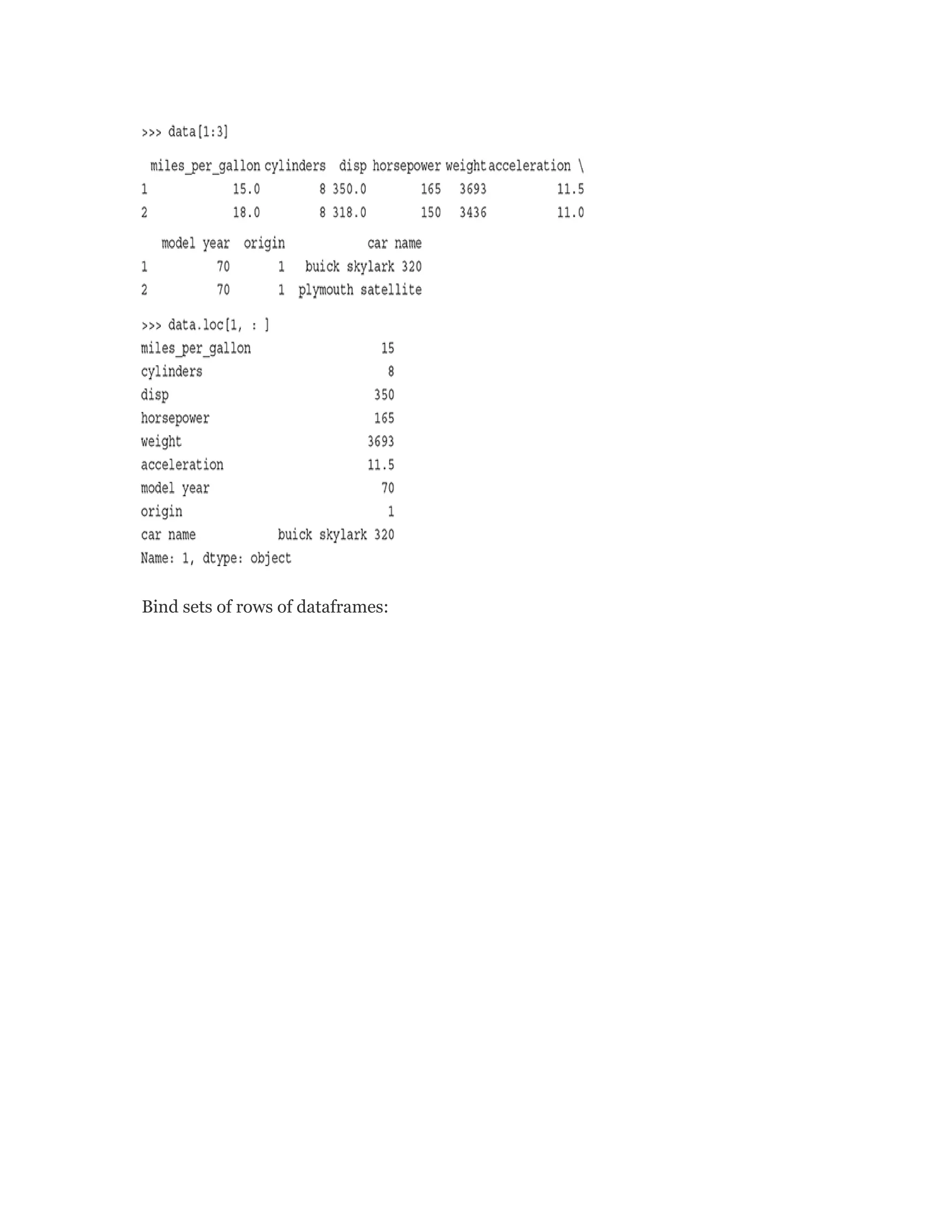
To extract specific rows:](https://image.slidesharecdn.com/mlsaikatdutt-221115120700-3df1a1af/75/ML_saikat-dutt-pdf-517-2048.jpg)

![There are six rows in the data set which have missing
values for the attribute ‘horsepower’. We will have to
remediate these rows before we proceed with the
modelling activities. We will do that shortly.
The easiest and most effective way to detect outliers is
from the box plot of the attributes. In the box plot,
outliers are very clearly highlighted. When we
explore the attributes using box plots in a short while, we
will have a clear view of this.
We can get the other statistical measure of the
attributes using the following Python commands from
the Numpy library:
>>> np.mean(data[[“mpg”]])
23.514573
>>> np.median(data[[“mpg”]])
23.0
>>> np.var(data[[“mpg”]])
60.936119](https://image.slidesharecdn.com/mlsaikatdutt-221115120700-3df1a1af/75/ML_saikat-dutt-pdf-525-2048.jpg)
![>>> np.std(data[[“mpg”]])
7.806159
Note:
Matplotlib is a plotting library for the Python
programming language which produces 2D plots to
render visualization and helps in exploring the data
sets. mat-plotlib.pyplot is a collection of command
style functions that make matplotlib work like
MATLAB
B.2.2 Basic plots for data exploration
In order to start using the library functions of
matplotlib, we need to include the library as follows:
>>> import matplotlib.pyplot as plt
Let’s now understand the different graphs that are
used for data exploration and how to generate them
using Python code.
We will use the “iris” data set, a very popular data set
in the machine learning world. This data set consists of
three different types of iris flower: Setosa, Versicolour,
and Virginica, the columns of the data set being - Sepal
Length, Sepal Width, Petal Length, and Petal Width. For
using this data set, we will first have to import the
Python library datasets using the code below.
>>> from sklearn import datasets
# import some data to play with
>>> iris = datasets.load_iris()
B.2.2.1 Box plot
>>> import matplotlib.pyplot as plt](https://image.slidesharecdn.com/mlsaikatdutt-221115120700-3df1a1af/75/ML_saikat-dutt-pdf-526-2048.jpg)
![>>> X = iris.data[:, :4]
>>> plt.boxplot(X)
>>> plt.show()
A box plot for each of the four predictors is generated as
shown in Figure B.2.
FIG. B.2 Box plot for an entire data set
As we can see, Figure B.2 gives the box plot for the
entire iris data set i.e. for all the features in the iris data
set, there is a component or box plot in the overall plot.
However, if we want to review individual features
separately, we can do that too using the following Python
command.
>>> plt.boxplot(X[:, 1])
>>> plt.show()
The output of the command i.e. the box plot of an
individual feature, sepal width, of the iris data set is
shown in Figure B.3.](https://image.slidesharecdn.com/mlsaikatdutt-221115120700-3df1a1af/75/ML_saikat-dutt-pdf-527-2048.jpg)
![FIG. B.3 Box plot for a specific feature
To find out the outliers of an attribute, we can use the
code below:
B.2.2.2 Histogram
>>> import matplotlib.pyplot as plt
>>> X = iris.data[:, :1]
>>> plt.hist(X)
>>> plt.xlabel(‘Sepal length’)
>>> plt.show()
The output of the command, i.e. the histogram of an
individual feature, Sepal Length, of the iris data set is
shown in Figure B.4.](https://image.slidesharecdn.com/mlsaikatdutt-221115120700-3df1a1af/75/ML_saikat-dutt-pdf-528-2048.jpg)
![FIG. B.4 Histogram for a specific feature
B.2.2.3 Scatterplot
>>> X = iris.data[:, :4] # We take the
first 4 features
>>> y = iris.target
>>> plt.scatter(X[:, 2], X[:, 0], c=y,
cmap=plt.cm.Set1, edgecolor=’k’)
>>> plt.xlabel(‘Petal length’)
>>> plt.ylabel(‘Sepal length’)
>>> plt.show()
The output of the command, i.e. the scatter plot for the
feature pair petal length and sepal length of the iris data
set is shown in Figure B.5.](https://image.slidesharecdn.com/mlsaikatdutt-221115120700-3df1a1af/75/ML_saikat-dutt-pdf-529-2048.jpg)
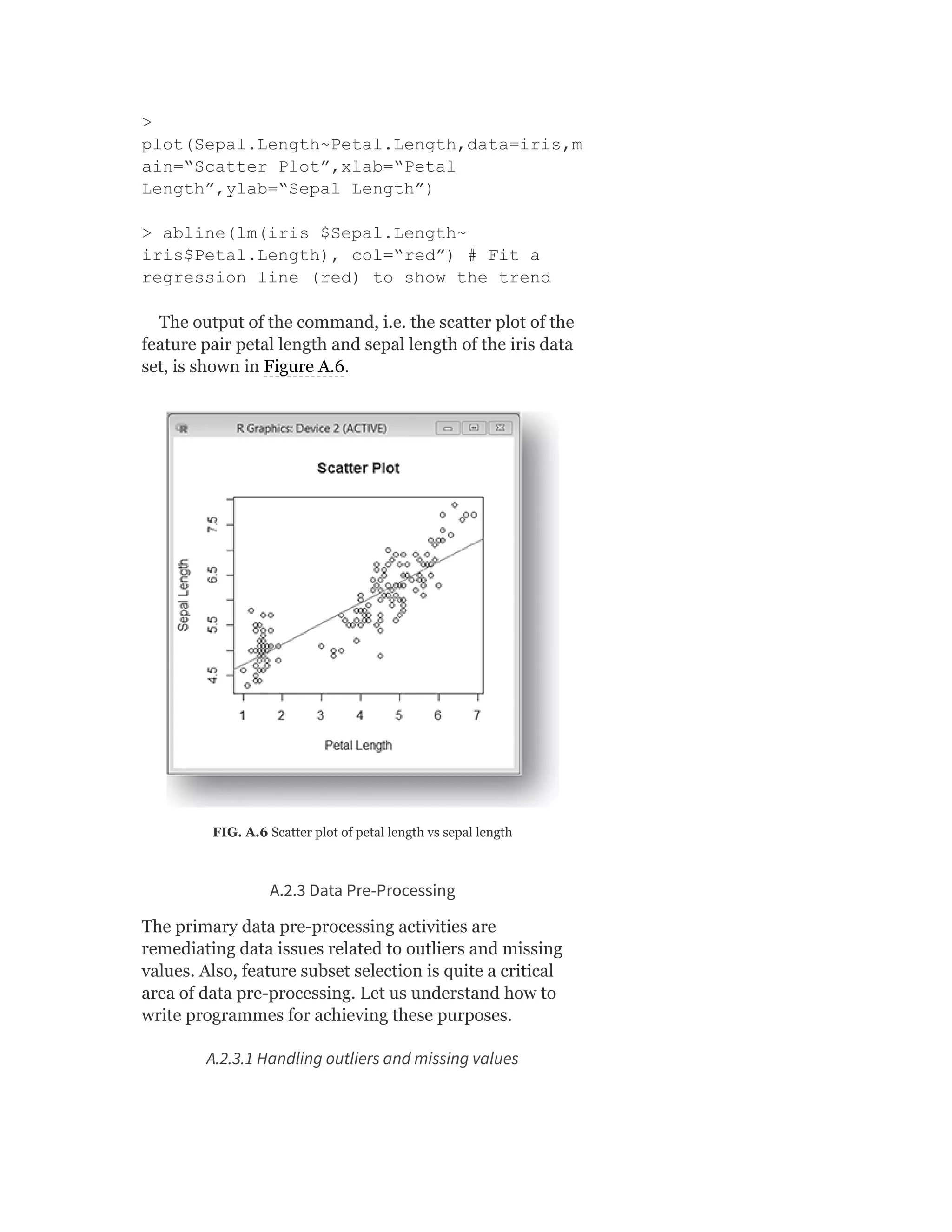
![FIG. B.5 Scatter plot of Petal Length vs. Sepal Length
B.2.3 Data pre-processing
The primary data pre-processing activities are
remediating data issues related to outliers and missing
values. Also, feature subset selection is quite a critical
area of data pre-processing. Let’s understand how to
write programs for achieving these purposes.
B.2.3.1 Handling outliers and missing values
As we saw in Chapter 2, the primary measures for
remediating outliers and missing values are
Removing specific rows containing outliers/missing values
Imputing the value (i.e. outliers/missing value) with a standard
statistical measure, e.g. mean or median or mode for that attribute
Estimate the value (i.e. outlier / missing value) based on value of the
attribute in similar records and replace with the estimated value.
Cap the values within 1.5 X IQR limits
B.2.3.1.1 Removing outliers / missing values
We have to first identify the outliers. We have already
seen in boxplots that outliers are clearly found out when
we draw the box plot of a specific attribute. Hence, we
can use the same concept as shown in the following code:
>>> outliers = plt.boxplot(X[:, 1])
[“fliers”][0].get_data()[1]](https://image.slidesharecdn.com/mlsaikatdutt-221115120700-3df1a1af/75/ML_saikat-dutt-pdf-530-2048.jpg)
![There is an alternate option too. As we know, outliers
have abnormally high or low value from other elements.
So the other option is to use threshold values to detect
outliers so that they can be removed. A sample code is
given below.
def find_outlier(ds, col):
quart1 = ds[col].quantile(0.25)
quart3 = ds[col].quantile(0.75)
IQR = quart3 - quart1 #Inter-quartile
range
low_val = quart1 - 1.5*IQR
high_val = quart3 + 1.5*IQR
ds = ds.loc[(ds[col] < low_val) |
(ds[col] > high_val)]
return ds
>>> outliers = find_outlier(data, “mpg”)
Then those rows can be removed using the code:
def remove_outlier(ds, col):
quart1 = ds[col].quantile(0.25)
quart3 = ds[col].quantile(0.75)
IQR = quart3 - quart1 #Interquartile
range
low_val = quart1 - 1.5*IQR
high_val = quart3 + 1.5*IQR
df_out = ds.loc[(ds[col] > low_val) &
(ds[col] < high_val)]
return df_out](https://image.slidesharecdn.com/mlsaikatdutt-221115120700-3df1a1af/75/ML_saikat-dutt-pdf-531-2048.jpg)
![>>> data = remove_outlier(data, “mpg”)
Rows having missing values can be removed using the
code:
>>> data.dropna(axis=0, how=’any’) #Remove
all rows where value of any column is
‘NaN’
B.2.3.1.2 Imputing standard values
The code for identification of outliers or missing values
will remain the same. For imputation, depending on
which statistical function is to be used for imputation,
code will be as follows:
Only the affected rows are identified and the value of
the attribute is transformed to the mean value of the
attribute.
>>> hp_mean = np.mean(data[‘horsepower’])
>>> imputedrows =
data[data[‘horsepower’].isnull()]
>>> imputedrows =
imputedrows.replace(np.nan, hp_mean)
Then the portion of the data set not having any missing
row is kept apart.
>>> missval_removed_rows =
data.dropna(subset=[‘horsepower’])
Then join back the imputed rows and the remaining part
of the data set.
>>> data_mod =
missval_removed_rows.append(imputedrows,
ignore_index=True)
In a similar way, outlier values can be imputed. Only
difference will be in identification of the relevant rows.
B.2.3.1.3 Capping of values](https://image.slidesharecdn.com/mlsaikatdutt-221115120700-3df1a1af/75/ML_saikat-dutt-pdf-532-2048.jpg)
![same machine learning program generates the same
set of results.
B.3.2 K-fold cross-validation
Let’s do k-fold cross-validation with 10 folds. For
creating the cross-validation, there are two options.
KFold function of either sklearn.cross_validation or
sklearn.model_ selection can be used as follows:
>>> import pandas as pd
>>> data = pd.read_csv(“auto-mpg.csv”)
# Option 1
>>> from sklearn.cross_validation import
KFold
>>> kf = KFold(data.shape[0], n_folds=10,
random_state=123)
>>> for train_index, test_index in kf:
data_train = data.iloc[train_index]
data_test = data.iloc[test_index]
# Option 2
>>> from sklearn.model_selection import
KFold
>>> kf = KFold(n_splits=10)
>>> for train, test in kf.split(data):
data_train = data.iloc[train_index]
data_test = data.iloc[test_index]
B.3.3 Bootstrap sampling
As discussed in Capter 3, bootstrap resampling is used to
generate samples of any given size from the training](https://image.slidesharecdn.com/mlsaikatdutt-221115120700-3df1a1af/75/ML_saikat-dutt-pdf-535-2048.jpg)
![data. It uses the concept of simple random sampling with
repetition. To generate bootstrap sample in Python,
resample function of sklearn.utils library can be used.
Below is a sample code
>>> import pandas as pd
>>> from sklearn.utils import resample
>>> data = pd.read_csv(“btissue.csv”)
>>> X = data.iloc[:,0:9]
>>> X
>>> resample(X, n_samples=200,
random_state=0) # Generates a sample of
size 200 (as mentioned in parameter
n_samples) with repetition …](https://image.slidesharecdn.com/mlsaikatdutt-221115120700-3df1a1af/75/ML_saikat-dutt-pdf-536-2048.jpg)
![B.3.4 Training the model
Once the model preparatory steps, like data holdout, etc.
are over, the actual training happens. The sklearn
framework in Python provides most of the models which
are generally used in machine learning. Below is a
sample code.
>>> from sklearn.tree import
DecisionTreeClassifier
>>> predictors = data.iloc[:,0:7] #
Segregating the predictors
>>> target = data.iloc[:,7] #
Segregating the target/class
>>> predictors_train, predictors_test,
target_train, target_test =
train_test_split(predictors, target,
test_size = 0.3, random_state = 123) #
Holdout of data
>>> dtree_entropy =
DecisionTreeClassifier(criterion =
“entropy”, random_state = 100,
max_depth=3, min_samples_leaf=5) #Model is
initialized](https://image.slidesharecdn.com/mlsaikatdutt-221115120700-3df1a1af/75/ML_saikat-dutt-pdf-537-2048.jpg)
![>>> import pandas as pd
>>> import numpy as np
>>> from sklearn.cluster import KMeans
>>> from sklearn.metrics.cluster import
v_measure_score
>>> data = pd.read_csv(“spine.csv”)
>>> data_woc = data.iloc[:,0:12] #
Stripping out the class variable from the
data set …
>>> data_class = data.iloc[:,12] #
Segregating the target / class variable …
>>> f1 =
data_woc[‘pelvic_incidence’].values
>>> f2 = data_woc[‘pelvic_radius’].values
>>> f3 = data_woc[‘thoracic_slope’].values
>>> X = np.array(list(zip(f1, f2, f3)))
>>> kmeans = KMeans(n_clusters = 2,
random_state = 123)
>>> model = kmeans.fit(X)
>>> cluster_labels = kmeans.predict(X)
>>> v_measure_score(cluster_labels,
data_class)
Output
0.12267025741680369
Silhouette Width
For calculating Silhouette Width, silhouette_score
function of sklearn. metrics library can be used for](https://image.slidesharecdn.com/mlsaikatdutt-221115120700-3df1a1af/75/ML_saikat-dutt-pdf-540-2048.jpg)
![calculating Silhouette width. Below is the code for
calculating Silhouette Width. A full implementation can
be found in a later section A.5.3.
>>> from sklearn.metrics import
silhouette_score
>>> sil = silhouette_score(X,
cluster_labels, metric =
’euclidean’,sample_size = len(data)) # “X”
is a feature matrix for the feature subset
selected for clustering and “data” is the
data set
B.4 FEATURE ENGINEERING
B.4.1 Feature construction
For doing feature construction, we can use pandas
library of Python. Following is a small code for
implementing feature construction.
>>> import pandas as pd
>>> room_length = [18, 20, 10, 12, 18, 11]
>>> room_breadth = [20, 20, 10, 11, 19,
10]
>>> room_type = [‘Big’, ‘Big’, ‘Normal’,
‘Normal’, ‘Big’, ‘Normal’]
>>> data = pd.DataFrame({‘Length’:
room_length, ‘Breadth’: room_ breadth,
‘Type’: room_type})
>>> data](https://image.slidesharecdn.com/mlsaikatdutt-221115120700-3df1a1af/75/ML_saikat-dutt-pdf-541-2048.jpg)
![B.4.1.1 Dummy coding categorical (nominal) variables:
get_dummies function of pandas library can be used to
dummy code categorical variables. Following is a sample
code for the same.
>>> import pandas as pd
>>> age = [18, 20, 23, 19, 18, 22]
>>> city = [‘City A’, ‘City B’, ‘City B’,
‘City A’, ‘City C’, ‘City B’]
>>> data = pd.DataFrame({‘age’: age,
‘city’: city})
>>> data](https://image.slidesharecdn.com/mlsaikatdutt-221115120700-3df1a1af/75/ML_saikat-dutt-pdf-542-2048.jpg)
![>>> dummy_features =
pd.get_dummies(data[‘city’])
>>> data_age = pd.DataFrame(data = data,
columns = [‘age’])
>>> data_mod =
pd.concat([data_age.reset_index(drop=True)
, dummy_ features], axis=1)
>>> data_mod
B.4.1.2 Encoding categorical (ordinal) variables:
LabelEncoder function of sklearn. preprocessing
library can be used to encode categorical variables.
Following is a sample code for the same.
>>> import pandas as pd
>>> from sklearn import preprocessing
>>> marks_science = [78,56,87,91,45,62]
>>> marks_maths = [75,62,90,95,42,57]
>>> grade = [‘B’,’C’,’A’,’A’,’D’,’B’]](https://image.slidesharecdn.com/mlsaikatdutt-221115120700-3df1a1af/75/ML_saikat-dutt-pdf-543-2048.jpg)
![>>> data = pd.DataFrame({‘Science marks’:
marks_science, ‘Maths marks’: marks_maths,
‘Total grade’: grade})
>>> data
# Option 1
>>> le = preprocessing.LabelEncoder()
>>> le.fit(data[‘Total grade’])
>>> data[‘Total grade’] =
le.transform(data[‘Total grade’])
>>> data
# Option 2
>>> target = data[‘Total
grade’].replace([‘A’,’B’,’C’ ,’D’],
[0,1,2,3])
>>> predictors = data.iloc[:, 0:2]
>>> data_mod =
pd.concat([predictors.reset_index(drop=Tru
e), target], axis=1)](https://image.slidesharecdn.com/mlsaikatdutt-221115120700-3df1a1af/75/ML_saikat-dutt-pdf-544-2048.jpg)
![B.4.1.3 Transforming numeric (continuous) features to
categorical features:
>>> import pandas as pd
>>> apartment_area = [4720, 2430, 4368,
3969, 6142, 7912]
>>> apartment_price =
[2360000,1215000,2184000,1984500,3071000,3
956000]
>>> data = pd.DataFrame({‘Area’:
apartment_area, ‘Price’: apartment_price})
>>> data
B.4.2 Feature extraction
B.4.2.1 Principal Component Analysis (PCA):
For doing principal component analysis or in other
words – to get the principal components of a set of
features in a data set, we can use PCA function of
sklearn.decomposition library. However, features](https://image.slidesharecdn.com/mlsaikatdutt-221115120700-3df1a1af/75/ML_saikat-dutt-pdf-545-2048.jpg)
![should be standardized (i.e. transform to unit scale with
mean = 0 and variance = 1), for which StandardScaler
function of sklearn. preprocessing library can be
used. Following is the code using the iris data set. PCA
should be applied on the predictors. The target / class
variable can be used to visualize the principal
components (Figure B.7).
>>> import pandas as pd
>>> import matplotlib.pyplot as plt
>>> from sklearn import datasets
>>> from sklearn.decomposition import PCA
>>> from sklearn.preprocessing import
StandardScaler
>>> iris = datasets.load_iris()
>>> predictors = iris.data[:, 0:4]
>>> target = iris.target
>>> predictors =
StandardScaler().fit_transform(predictors)
# Standardizing the features
>>> pca = PCA(n_components=2)
>>> princomp =
pca.fit_transform(predictors)
>>> princomp_ds = pd.DataFrame(data =
princomp, columns = [‘PC 1’, ‘PC 2’])
>>> princomp_ds](https://image.slidesharecdn.com/mlsaikatdutt-221115120700-3df1a1af/75/ML_saikat-dutt-pdf-546-2048.jpg)

![FIG. B.7 Principal components of iris data set
B.4.2.2 Singular Value Decomposition (SVD):
We have seen in Chapter 4 that singular value
decomposition of a matrix A (m X n) is a factorization of
the form:
A = U∑V = UsV (representing ∑ or Sigma by “s”)
For implementing singular value decomposition in
Python, we can use svd function of scipy.linalg library.
Following is the code using the iris data set.
>>> import pandas as pd
>>> from sklearn import datasets
>>> from scipy.linalg import svd
>>> iris = datasets.load_iris()
>>> predictors = iris.data[:, 0:4]
>>> U, s, VT = svd(predictors)
>>> print(U)
T](https://image.slidesharecdn.com/mlsaikatdutt-221115120700-3df1a1af/75/ML_saikat-dutt-pdf-549-2048.jpg)
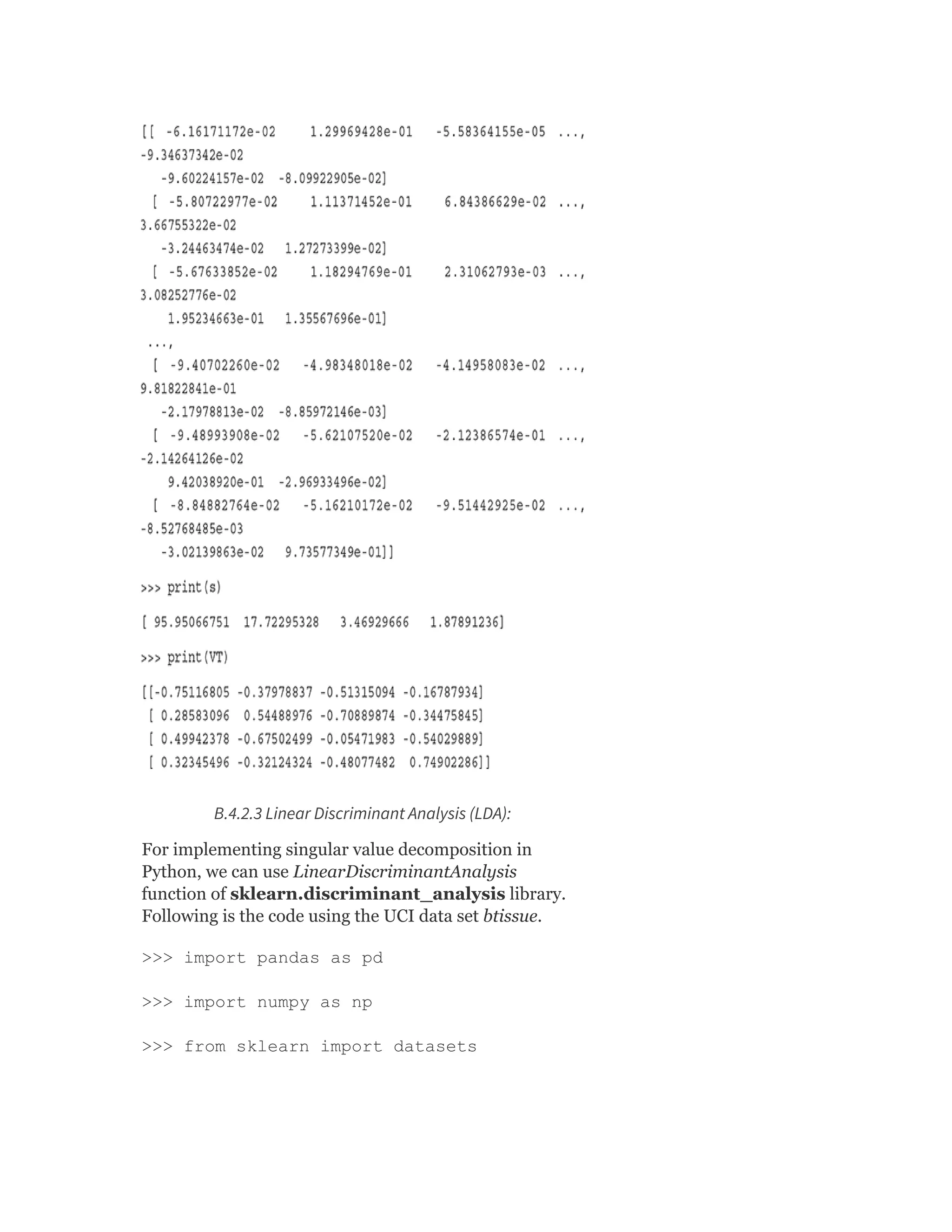
![>>> from sklearn.discriminant_analysis
import LinearDiscriminantAnalysis
>>> from sklearn.utils import column_or_1d
>>> data = pd.read_csv(“btissue.csv”)
>>> X = data.iloc[:,0:9]
>>> y = column_or_1d(data[‘class’],
warn=True) #To generate 1d array,
column_or_1d has been used …
>>> clf = LinearDiscriminantAnalysis()
>>> lda_fit = clf.fit(X, y)
>>> print(lda_fit)
LinearDiscriminantAnalysis(n_components=No
ne, priors=None,
shrinkage=None,solver=’svd’,
store_covariance=False, tol=0.0001)
>>> pred = clf.predict([[1588.000000,
0.085908, -0.086323, 516.943603,
12895.342130, 25.933331, 141.722204,
416.175649, 1452.331924]])
>>> print(pred)
[‘con’]
B.4.3 Feature subset selection
Feature subset selection is a topic of intense research.
There are many approaches to select a subset of features
which can improve model performance. It is not possible
to cover all such approaches as a part of this text.
However, sklearn.feature_selection module can be used
for applying basic feature selection. There are multiple
options of feature selection offered by the module, one of
which is presented below:
>>> import pandas as pd](https://image.slidesharecdn.com/mlsaikatdutt-221115120700-3df1a1af/75/ML_saikat-dutt-pdf-551-2048.jpg)
![>>> import numpy as np
>>> from sklearn.feature_selection import
SelectKBest
>>> from sklearn.feature_selection import
chi2
>>> data = pd.read_csv(“apndcts.csv”)
>>> predictors = data.iloc[:,0:7] #
Seggretating the predictor variables …
>>> target = data.iloc[:,7] #
Seggretating the target / class variable …
>>> test = SelectKBest(chi2, k=2)
>>> fit = test.fit(predictors, target)
>>> features = fit.transform(predictors)
>>> print(predictors.columns)
>>> np.set_printoptions(precision=3)
>>> print(fit.scores_)
Output:
Index([‘At1’, ‘ At2’, ‘ At3’, ‘ At4’, ‘
At5’, ‘ At6’, ‘ At7’], dtype=’object’)
Scores for each feature:
[ 1.771 1.627 2.391 1.084 1.673 1.647
2.236]
B.5 MACHINE LEARNING MODELS
B.5.1 Supervised learning - classification
In the chapter 6, 7, and 8, conceptual overview of
different supervised learning algorithms has been
presented. Now, you will get to know, how to implement](https://image.slidesharecdn.com/mlsaikatdutt-221115120700-3df1a1af/75/ML_saikat-dutt-pdf-552-2048.jpg)
![them using Python. For the sake of simplicity, we have
tried to keep the code for implementing each of the
algorithms as consistent as possible. Also, we have used
benchmark data sets from UCI repository (will also keep
it available online).
B.5.1.1 Naive bayes classifier:
For Naive Bayes classifier implementation, GaussianNB
library of sklearn.naive_ bayes has been used. The
full code for the implementation is given below.
>>> import pandas as pd
>>> from sklearn.model_selection import
train_test_split
>>> from sklearn.metrics import
accuracy_score
>>> from sklearn.naive_bayes import
GaussianNB
>>> data = pd.read_csv(“apndcts.csv”)
>>> predictors = data.iloc[:,0:7] #
Segregating the predictor variables …
>>> target = data.iloc[:,7] #
Segregating the target / class variable …
>>> predictors_train, predictors_test,
target_train, target_test =
train_test_split(predictors, target,
test_size = 0.3, random_state = 123)
>>> gnb = GaussianNB()
# First train model / classifier with the
input dataset (training data part of it)
>>> model = gnb.fit(predictors_train,
target_train)
# Make prediction using the trained model](https://image.slidesharecdn.com/mlsaikatdutt-221115120700-3df1a1af/75/ML_saikat-dutt-pdf-553-2048.jpg)
![>>> prediction =
model.predict(predictors_test)
# Time to check the prediction accuracy …
>>> accuracy_score(target_test,
prediction, normalize = True)
Output Accuracy:
0.90625
B.5.1.2 kNN classifier:
k-Nearest Neighbour (kNN) classifier is implemented
through KNeighborsClassifier library of sklearn.
neighbors. The full code for the implementation is
given below.
>>> import pandas as pd
>>> from sklearn.model_selection import
train_test_split
>>> from sklearn.metrics import
accuracy_score
>>> from sklearn.neighbors import
KNeighborsClassifier
>>> data = pd.read_csv(“apndcts.csv”)
>>> predictors = data.iloc[:,0:7] #
Seggretating the predictor variables …
>>> target = data.iloc[:,7] #
Seggretating the target / class variable …
>>> predictors_train, predictors_test,
target_train, target_test =
train_test_split(predictors, target,
test_size = 0.3, random_state = 123)
>>> nn = KNeighborsClassifier(n_neighbors
= 3) # Instantiate the model with 3
neighbors …](https://image.slidesharecdn.com/mlsaikatdutt-221115120700-3df1a1af/75/ML_saikat-dutt-pdf-554-2048.jpg)
![# First train model / classifier with the
input dataset (training data part of it)
>>> model = nn.fit(predictors_train,
target_train)
# Time to check the prediction accuracy …
>>> nn.score(predictors_test, target_test)
Output Accuracy:
0.875
B.5.1.3 Decision tree classifier:
Decision Tree classifier can be implemented using
DecisionTreeClassifier library of sklearn. tree has been
used. The full code for the implementation is given
below.
>>> import pandas as pd
>>> from sklearn.model_selection import
train_test_split
>>> from sklearn.metrics import
accuracy_score
>>> from sklearn.tree import
DecisionTreeClassifier
>>> data = pd.read_csv(“apndcts.csv”)
>>> predictors = data.iloc[:,0:7] #
Seggretating the predictor variables …
>>> target = data.iloc[:,7] #
Seggretating the target / class variable …
>>> predictors_train, predictors_test,
target_train, target_test =
train_test_split(predictors, target,
test_size = 0.3, random_state = 123)](https://image.slidesharecdn.com/mlsaikatdutt-221115120700-3df1a1af/75/ML_saikat-dutt-pdf-555-2048.jpg)
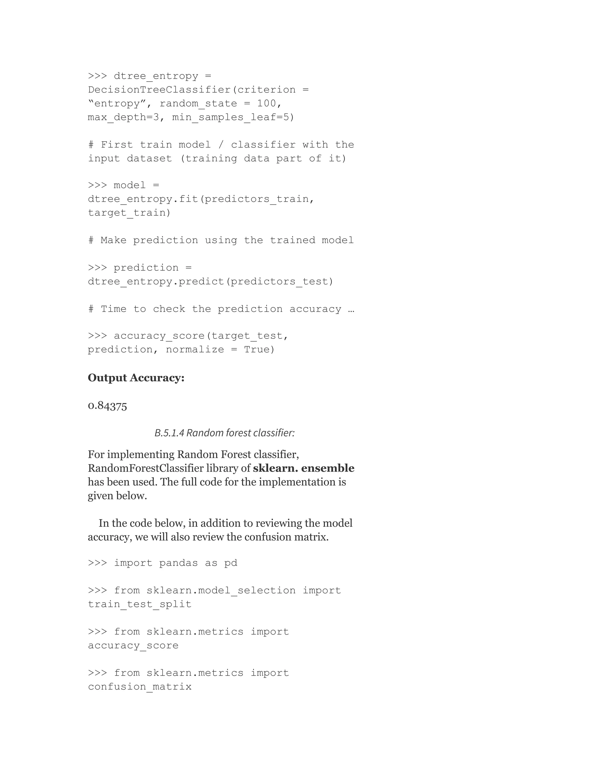
![>>> from sklearn.ensemble import
RandomForestClassifier
>>> data = pd.read_csv(“apndcts.csv”)
>>> predictors = data.iloc[:,0:7] #
Segregating the predictor variables …
>>> target = data.iloc[:,7] #
Segregating the target / class variable …
>>> predictors_train, predictors_test,
target_train, target_test =
train_test_split(predictors, target,
test_size = 0.3, random_state = 123)
>>> rf = RandomForestClassifier()
# First train model / classifier with the
input dataset (training data part of it)
>>> model = rf.fit(predictors_train,
target_train)
# Make prediction using the trained model
>>> prediction =
rf.predict(predictors_test)
# Time to check the prediction accuracy…
>>> accuracy_score(target_test,
prediction, normalize = True)
# And this time let’s look at the
confusion matrix too…
>>> confusion_matrix(target_test,
prediction)
Output Accuracy:
Accuracy ➠ 0.875
Confusion matrix ➠ array([[25, 0],](https://image.slidesharecdn.com/mlsaikatdutt-221115120700-3df1a1af/75/ML_saikat-dutt-pdf-557-2048.jpg)
![[ 4, 3]], dtype=int64)
B.5.1.5 SVM Classifier:
For implementing Random Forest classifier, svm library
of sklearn framework has been used. The full code for
the implementation is given below.
>>> import pandas as pd
>>> from sklearn.model_selection import
train_test_split
>>> from sklearn.metrics import
accuracy_score
>>> from sklearn import svm
>>> data = pd.read_csv(“apndcts.csv”)
>>> predictors = data.iloc[:,0:7] #
Seggretating the predictor variables …
>>> target = data.iloc[:,7] #
Seggretating the target / class variable …
>>> predictors_train, predictors_test,
target_train, target_test =
train_test_split(predictors, target,
test_size = 0.3, random_state = 123)
>>> svm = svm.SVC(kernel=’linear’) # SVC
with linear kernel
# First train model / classifier with the
input dataset (training data part of it)
>>> model = svm.fit(predictors_train,
target_train)
# Make prediction using the trained model
>>> prediction =
svm.predict(predictors_test)
# Time to check the prediction accuracy …](https://image.slidesharecdn.com/mlsaikatdutt-221115120700-3df1a1af/75/ML_saikat-dutt-pdf-558-2048.jpg)
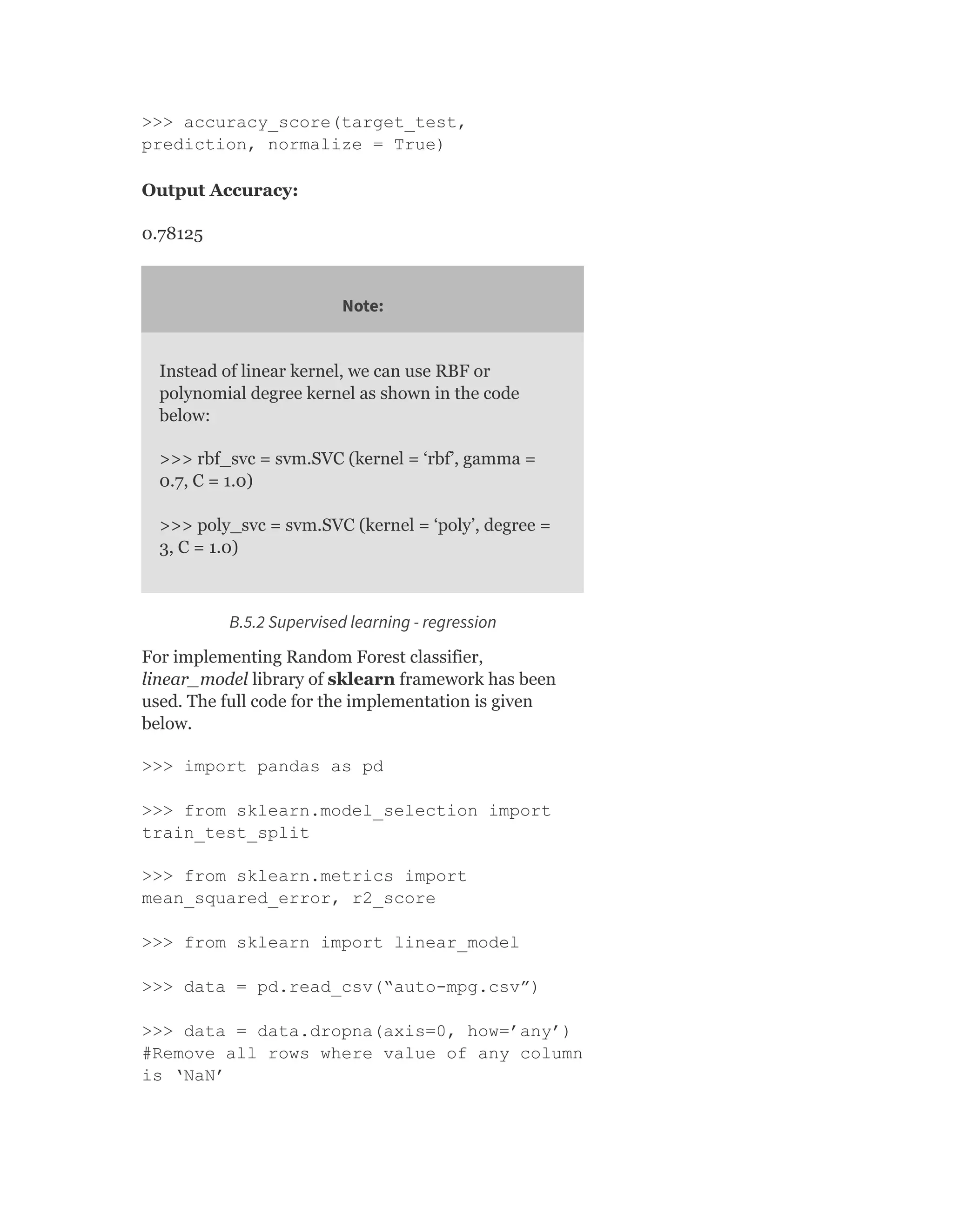
![>>> predictors = data.iloc[:,1:7] #
Seggretating the predictor variables …
>>> target = data.iloc[:,0] #
Seggretating the target / class variable …
>>> predictors_train, predictors_test,
target_train, target_test =
train_test_split(predictors, target,
test_size = 0.3, random_state = 123)
>>> lm = linear_model.LinearRegression()
# First train model / classifier with the
input dataset (training data part of it)
>>> model = lm.fit(predictors_train,
target_train)
# Make prediction using the trained model
>>> prediction =
model.predict(predictors_test)
>>> mean_squared_error(target_test,
prediction)
>>> r2_score(target_test, prediction)
Output Accuracy:
Mean squared error ➠ 20.869480380073597
R score ➠ 0.63425991602097787
B.5.3 Unsupervised learning
For the implementation of kmeans algorithm, KMeans
function of sklearn.cluster library has been used. Also,
since silhouette width is a more generic performance
measure, it has been used here. silhouette_score
function of sklearn. metrics library has been used for
calculating Silhouette width. The full code for the
implementation is given below (Figure B.8).
>>> import pandas as pd
2](https://image.slidesharecdn.com/mlsaikatdutt-221115120700-3df1a1af/75/ML_saikat-dutt-pdf-560-2048.jpg)
![>>> import numpy as np
>>> import matplotlib.pyplot as plt
>>> from mpl_toolkits.mplot3d import
Axes3D
>>> from sklearn.cluster import KMeans
>>> from sklearn.metrics import
silhouette_score
>>> data = pd.read_csv(“spinem.csv”)
>>> f1 = data[‘pelvic_incidence’].values
>>> f2 = data[‘pelvic_radius’].values
>>> f3 = data[‘thoracic_slope’].values
>>> X = np.array(list(zip(f1, f2, f3)))
>>> kmeans = KMeans(n_clusters = 3,
random_state = 123)
>>> model = kmeans.fit(X)
>>> cluster_labels = kmeans.predict(X)
>>> C = kmeans.cluster_centers_
>>> sil = silhouette_score(X,
cluster_labels,
metric=’euclidean’,sample_size =
len(data))
>>> print(C)
>>> print(sil)
#For 2-D plot of the data points along
with the centroids …
>>> fig = plt.figure()](https://image.slidesharecdn.com/mlsaikatdutt-221115120700-3df1a1af/75/ML_saikat-dutt-pdf-561-2048.jpg)
![>>> plt.scatter(X[:, 0], X[:, 1])
>>> plt.scatter(C[:, 0], C[:, 1],
marker=’*’, s=1000)
#For 3-D plot of the data points along
with the centroids …
>>> fig = plt.figure()
>>> ax = Axes3D(fig)
>>> ax.scatter(X[:, 0], X[:, 1], X[:, 2])
>>> ax.scatter(C[:, 0], C[:, 1], C[:, 2],
marker=’*’, c=’#050505’, s=1000)
Output Accuracy:
Centroids:
[[ 46.42903837 124.47018491 13.26250567]
[ 80.49567418 120.00557969 12.78133516]
[ 62.59438009 103.64870812 13.03697051]]
Silhouette width:
0.352350820437](https://image.slidesharecdn.com/mlsaikatdutt-221115120700-3df1a1af/75/ML_saikat-dutt-pdf-562-2048.jpg)
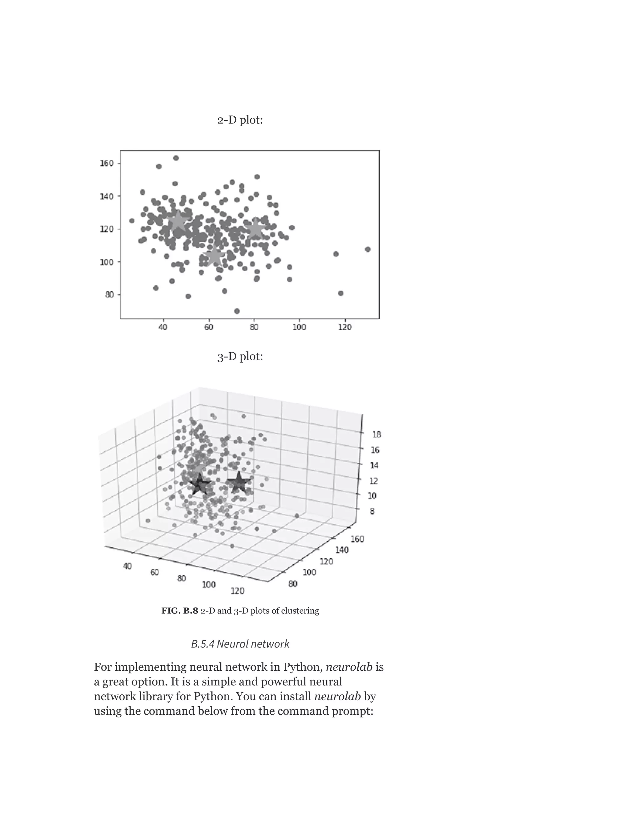
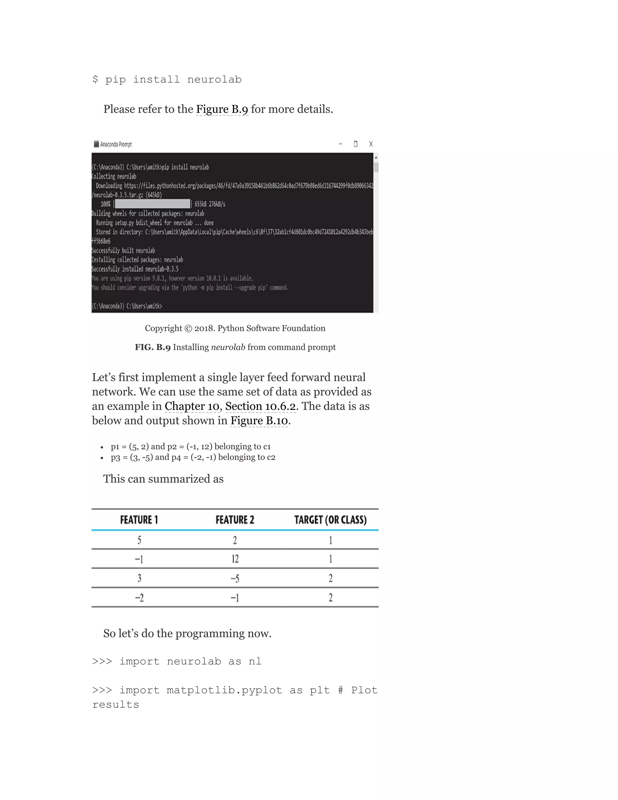
![>>> input = [[5, 2], [-1, 12], [3, -5],
[-2, -1]]
>>> target = [[1], [1], [2], [2]]
# Create single layer neural net with 2
inputs and 1 neuron
>>> net = nl.net.newp([[-2, 12],[1, 2]],
1) # Function newp is for implementing
single layer perceptron …
>>> error = net.train(input, target,
epochs=10, show=10, lr=0.1)
>>> plt.plot(error)
>>> plt.xlabel(‘Epoch number’)
>>> plt.ylabel(‘Train error’)
>>> plt.grid()
>>> plt.show()
FIG. B.10 Epoch number vs. error in a single-layer NN
Next let’s implement a multi layer feed forward neural
network. We can have multiple hidden layers in this case.
In this case, we will use multi layer neural network as a
regressor i.e. to predict a continuous variable. A set of 75](https://image.slidesharecdn.com/mlsaikatdutt-221115120700-3df1a1af/75/ML_saikat-dutt-pdf-565-2048.jpg)
![values of predictor variable is first generated within a
specified range. The corresponding target values are
generated using the equation y = 4x + 7.6 and
normalized. Using these set of points, a multi layer
neural network is trained. Then using the trained model,
predictions are generated and compared with the actual
data points generated from the regression function.
>>> import neurolab as nl
>>> import matplotlib.pyplot as plt
# Create train samples assuming minimum
value = -2, maximum value = 2 and number
of training points = 75
>>> minm_val = -2
>>> maxm_val = 2
>>> no_points = 75
>>> x = np.linspace(minm_val, maxm_val,
no_points)
>>> y = 4*np.square(x) + 7.6
>>> y /= np.linalg.norm(y)
>>> input_data = x.reshape(no_points,1)
>>> target = y.reshape(no_points,1)
# Create network with 2 hidden layers -
with 12 neurons in the first layer and 8
neurons in the second layer.
# Task is to predict the value, so the
output layer will contain 1 neuron …
>>> net = nl.net.newff([[minm_val,
maxm_val]],[12, 8, 1])
# Then the training algorithm is set to
gradient descent …
2](https://image.slidesharecdn.com/mlsaikatdutt-221115120700-3df1a1af/75/ML_saikat-dutt-pdf-566-2048.jpg)
![>>> net.trainf = nl.train.train_gd
# Now do the real training
>>> error = net.train(input_data, target,
epochs=2000, show=100, goal=0.01)
# Simulate network to generate prediction
…
>>> output_data = net.sim(input_data)
>>> pred_val =
output_data.reshape(no_points)
# Plotting the results …
>>> plt.figure()
>>> plt.plot(error)
>>> plt.xlabel(‘Epoch number’)
>>> plt.ylabel(‘Train error’)
>>> plt.grid()
>>> plt.show()
>>> x_dash = np.linspace(minm_val,
maxm_val, no_points*2)
>>> y_dash =
net.sim(x_dash.reshape(x_dash.size,1)).res
hape(x_ dash.size)
>>> plt.figure()
>>> plt.plot(x_dash, y_dash, ‘.’, x, y,
‘+’, x, pred_val, ‘p’)
>>> plt.legend([‘Actual’, ‘Predicted’])
>>> plt.title(‘Actual vs predicted’)](https://image.slidesharecdn.com/mlsaikatdutt-221115120700-3df1a1af/75/ML_saikat-dutt-pdf-567-2048.jpg)