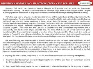
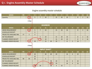
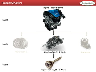
1. Phil Harris, the Production Control Manager at Brunswick Motors, wants to illustrate time-phased requirements planning using an example with the company's Model 1000 engine. He prepares a master schedule for the engine over 12 weeks. 2. Phil considers two components for the engine, the gear box and input shaft. He includes their manufacturing lead times and product structure. The gear box takes 2 weeks to produce and the input shaft takes 3 weeks. 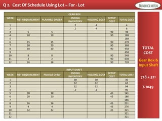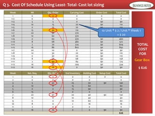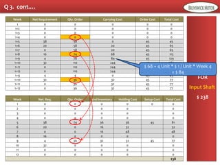3. Phil plans to use MRP worksheets and make assumptions about starting inventory levels and scheduled deliveries for the gear box and input shaft. He will calculate net requirements and planned order releases using lot-for-lot ordering.

1. BRUSNSWICK MOTORS, INC
AN INTRODUCTORY CASE FOR MRP

2. Presented By
Pravin P. Narwade
Dr. V. N. Bedekar Institute Of Management Studies, Thane
(University Of Mumbai)

3. BRUNSWICK MOTORS, INC - AN INTRODUCTORY CASE FOR MRP
Recently, Phil Harris, the Production Control Manager at Brunswick read an article on time-phased
requirements planning. He was curious about how this technique might work in scheduling Brunswick's engine
assembly operations and decided to prepare an example to illustrate the of time-phased requirements planning.
Phil's first step was to prepare a master schedule for one of the engine types produced by Brunswick, the
Model 1000 engine. The schedule indicates the number of units of the Model 1000 engine to be assembled during
each week over the next twelve weeks and is shown below. Next, Phil decided to simplify his requirements
planning example by considering only two of the many components which are needed to complete the assembly
of the Model 1000 engine. These two components, the Gear Box and the Input Shaft, are shown in the Product
Structure Diagram. Phil noted that the Gear Box is assembled by the Sub-Assembly Department, and is
subsequently sent to the main engine assembly line. The Input Shaft is one of several component parts
manufactured by Brunswick that are needed to produce a Gear Box sub-assembly. Thus, levels 0, 1, and 2 are
included in Product Structure Diagram to indicate the three manufacturing stages that are involved in producing
an engine: The Engine Assembly Department, the Sub-Assembly Department, and the Machine Shop.
The manufacturing lead times required to produce the Gear Box and the Input Shaft components are also
indicated in the product structure diagram. Note that two weeks are required to produce a batch of Gear Boxes
and that all of the Gear Boxes must be delivered to the assembly line parts stockroom before Monday morning of
the week in which they are to be used. Likewise, it takes three weeks to produce a lot of Input Shafts, and all of
the shafts that are needed for the production of Gear Boxes in a given week must be delivered to the Sub
Assembly Department stockroom before Monday morning of that week.
In preparing the MRP example, Phil planned to use the worksheets and to make the following assumptions:
1. Seventeen Gear Boxes are on hand at the beginning of week 1 and five Gear Boxes are currently on order to
be delivered at the start of week 2.
2. Forty Input Shafts are on hand at the start of week 1 and 22 scheduled for delivery at the beginning of week 2 .

4. BURNSWICK MOTORS, INC - AN INTRODUCTORY CASE FOR MRP
Assignment
1. Initially, assume that Phil wants to minimize his inventory requirements. Assume that each order will be on the
for what is required for a single period. Using the following forms, calculate the net requirement and planned
order releases for the gearbox and input shafts. Assume that lot sizing is done using lot-for-lot.
2. Phil would like to consider the cost that his accountants are currently using for inventory carrying and setup
for the gearboxes and input shafts. These costs are as follows:
Part Cost
Gear Box Setup = $ 90/order
Inventory carrying cost = $ 2 /unit/week
Input Shaft Setup = $ 45/order
Inventory carrying cost = $ 1 /unit/week
Given the cost structure, evaluate the cost of schedule form (1). Assume inventory is valued at the end of each
week.
3. Calculate a schedule using least-total-cost lot sizing. What are the savings with this new schedule ?
Week 1 2 3 4 5 6 7 8 9 10 11 12
Demand 15 5 7 10 15 20 10 8 2 16
Ref. Book : | Operations & Supply Management | 12th Edition
| Rechard B. Chase | Ravi Shankar | F. Robert Jacobs | Nicholas J. Aquilano
TATA Mc Graw Hill Education
Mc
Graw
Hill
Education
Model 1000 master schedule

5. Definitions Of Terms
Item : Name or number for the item being scheduled
Low level code : The lowest level of the item on the product structure file
Lot size : Order multiplies of quantity
Lead time : The time from when an order is placed to when it is required
PD : Past due time or Bucket order behind schedule
Gross requirement : Total expected demand for an item in a time period.
Scheduled receipt : Material already ordered
Projected available balance : Expected ending inventory.
Net requirement : The actual amount needed in each time period.
Planned order receipt : Quantity expected to be received by the beginning of the period
or Net requirements adjusted for lot size.
Planned order releases : Planned order receipts offset by lead time.

6. Formulae
Gross requirement = Forecasted demand period by period
Net requirement (t) = Gross requirement (t) – Projected inventory (t - 1) – Scheduled receipt (t)
Projected inventory (t) = Projected inventory (t - 1) + Scheduled receipt (t) +
Planned order receipt (t) – Gross requirement (t)
Planned order releases (t - LT) = Planned order receipt (t)
Total cost = Carrying cost + Setup cost
(Carrying cost = Holding Cost, Setup cost = Ordering Cost)
t = current .
t -1 = previous .
LT = lead time .

7. Input Shaft (2), LT = 3 Week
Engine : Model 1000
Transmission Gearbox (1), LT= 2 Week Crank case
Level 0
Level 1
Level 2
Product Structure

8. GEARBOX
WEEKS PD 1 2 3 4 5 6 7 8 9 10 11 12
GROSS REQUIREMENT 15 5 7 10 15 20 10 8 2 16
SCHEDULED RECEIPT 5
PROJECTED AVAILABLE BAL. 17 2 2
NET REUIREMENT 5 10 15 20 10 8 2 16
PLANNED ORDER RECEIPT 5 10 15 20 10 8 2 16
PLANNED ORDER RELEASE 5 10 15 20 10 8 2 16
WEEKS PD 1 2 3 4 5 6 7 8 9 10 11 12
Quantity 15 5 7 10 15 20 10 8 2 16
INPUT SHAFT
WEEKS PD 1 2 3 4 5 6 7 8 9 10 11 12
GROSS REQUIREMENT 10 20 30 40 20 16 4 32
SCHEDULED RECEIPT 22
PROJECTED AVAILABLE BAL. 40 30 32 2
NET REUIREMENT 38 20 16 4 32
PLANNED ORDER RECEIPT 38 20 16 4 32
PLANNED ORDER RELEASE 38 20 16 4 32
2 Times
1 Time
Engine assembly master schedule
Q 1. Engine Assembly Master Schedule

9. Q 2. Cost Of Schedule Using Lot – For - Lot
GEAR BOX
WEEK
NET REQUIREMENT PLANNED ORDER
ENDING
INVENTORY
HOLDING COST
SETUP
COST
TOTAL COST
1 2 4 4
2 2 4 8
3 5 5 90 98
4 10 10 90 188
5 188
6 15 15 90 278
7 20 20 90 368
8 10 10 90 458
9 458
10 8 8 90 548
11 2 2 90 638
12 16 16 90 728
INPUT SHAFT
WEEK NET REQUIREMENT Planned Order
ENDING
INVENTORY
HOLDING COST
SETUP
COST
TOTAL COST
1 30 30 30
2 32 32 62
3 32 32 94
4 2 2 96
5 38 38 45 141
6 20 20 45 186
7 186
8 16 16 45 231
9 4 4 45 276
10 32 32 45 321
11 321
12 321
TOTAL
COST
728 + 321
$ 1049
Gear Box &
Input Shaft

10. Q 3. Cost Of Schedule Using Least- Total- Cost lot sizing
Week NR Qty. Order Carrying Cost Order Cost Total Cost
1 0 0 0 0 0
1=2 0 0 0 0 0
1=3 5 5 0 90 90
1=4 10 15 20 90 110
1=5 0 15 20 90 110
1=6 15 30 110 90 200
1=7 20 50 270 90 360
1=8 10 60 370 90 460
1=9 0 60 370 90 460
1=10 8 68 482 90 572
1=11 2 70 514 90 604
1=12 16 86 802 90 892
1=7 20 20 0 90 90
1=8 10 30 20 90 110
1=9 0 30 20 90 110
1=10 8 38 68 90 158
1=11 2 40 84 90 174
1=12 16 56 244 90 334
1=12 16 16 0 90 90
Week Net. Req. Qty. Order End Inventory Holding Cost Setup Cost Total Cost
1 0 0 0 0 0 0
2 0 0 0 0 0
3 5 30 25 50 90 140
4 10 0 15 60 60
5 0 0 15 90 90
6 15 0 0 0 0
7 20 40 20 40 90 130
8 10 0 10 40 40
9 0 0 10 60 60
10 8 0 2 16 16
11 2 0 0 0 0
12 16 16 0 0 90 90
626
TOTAL
COST
FOR
$ 626
Gear Box
10 Unit * $ 2 / Unit * Week 1
= $ 20

11. Q 3. cont.…
TOTAL
COST
FOR
$ 238
Week Net Requirement Qty. Order Carrying Cost Order Cost Total Cost
1 0 0 0 0 0
1=2 0 0 0 0 0
1=3 0 0 0 0 0
1=4 0 0 0 0 0
1=5 38 38 0 45 45
1=6 20 58 20 45 65
1=7 0 58 20 45 65
1=8 16 74 68 45 113
1=9 4 78 84 45 129
1=10 32 110 244 45 289
1=11 0 110 244 45 289
1=12 0 110 244 45 289
1=9 4 4 0 45 45
1=10 32 36 32 45 77
1=11 0 36 32 45 77
1=12 0 36 32 45 77
Week Net. Req. Qty. Order End Inventory Holding Cost Setup Cost Total Cost
1 0 0 0 0 0 0
2 0 0 0 0 0
3 0 0 0 0 0
4 0 0 0 0 0
5 38 74 36 36 45 81
6 20 0 16 32 32
7 0 0 16 48 48
8 16 0 0 0 0
9 4 36 32 32 45 77
10 32 0 0 0 0
11 0 0 0 0 0
12 0 0 0 0 0
238
Input Shaft
$ 68 + 4 Unit * $ 1 / Unit * Week 4
= $ 84

12. Conclusion
Least Total Cost Method (LTC) : a dynamic lot sizing technique that calculates the order quantity
by comparing the carrying cost and the setup cost for various lot sizes and then selects the lot in
which these are most nearly equal.
Total cost using lot -- for – lot
Gear Box = 728
Input Shaft = 321
Total Cost = 1049
Total cost using least total cost lot sizing
Gear Box = 626
Input Shaft = 238
Total Cost = 864
Total Cost Saving
$ 1049
$ 0864
$ 0185

13. Thank You