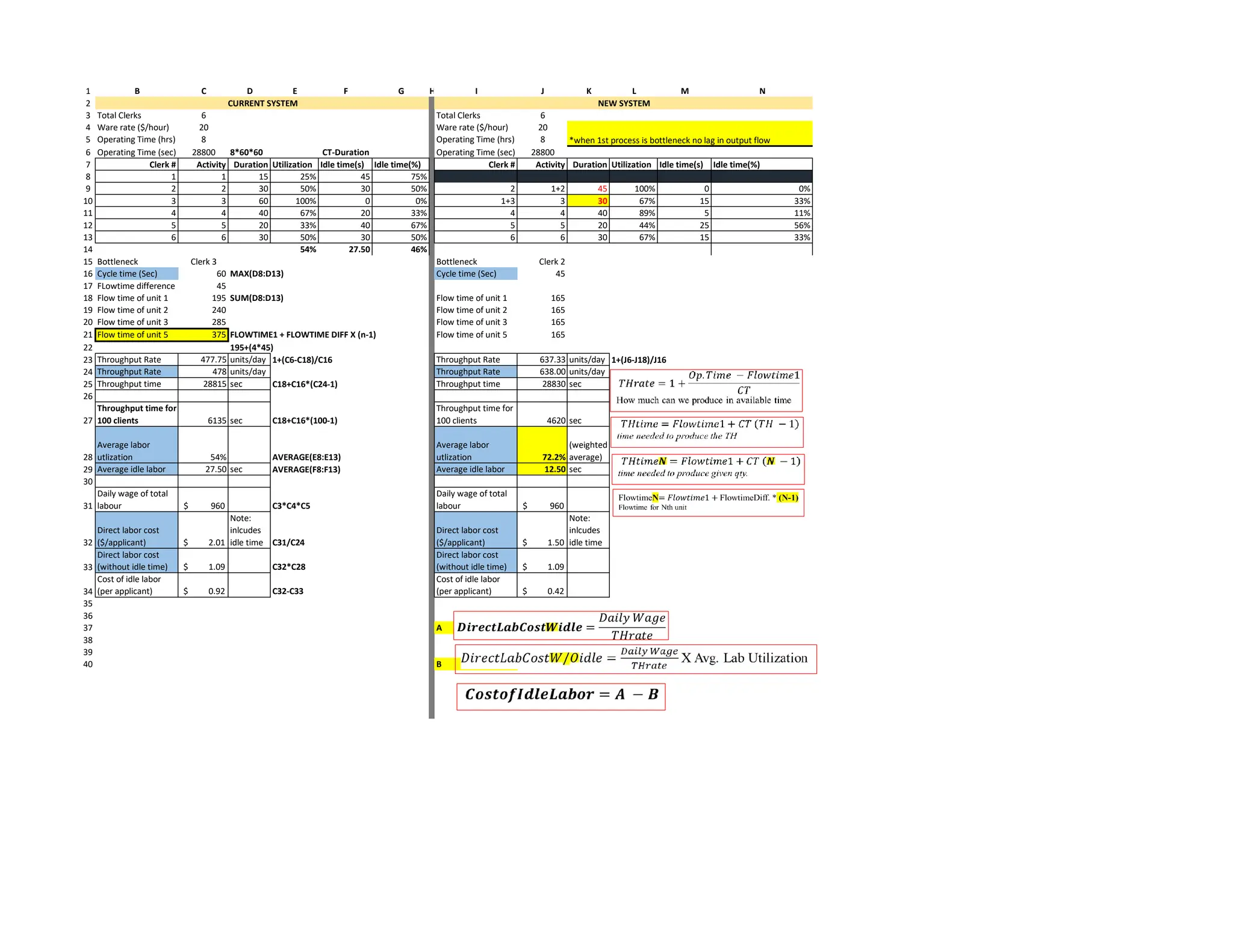
1 B C D E F G H I J K L M N
2
3 Total Clerks 6 Total Clerks 6
4 Ware rate ($/hour) 20 Ware rate ($/hour) 20
5 Operating Time (hrs) 8 Operating Time (hrs) 8
6 Operating Time (sec) 28800 8*60*60 CT-Duration Operating Time (sec) 28800
7 Clerk # Activity Duration Utilization Idle time(s) Idle time(%) Clerk # Activity Duration Utilization Idle time(s) Idle time(%)
8 1 1 15 25% 45 75%
9 2 2 30 50% 30 50% 2 1+2 45 100% 0 0%
10 3 3 60 100% 0 0% 1+3 3 30 67% 15 33%
11 4 4 40 67% 20 33% 4 4 40 89% 5 11%
12 5 5 20 33% 40 67% 5 5 20 44% 25 56%
13 6 6 30 50% 30 50% 6 6 30 67% 15 33%
14 54% 27.50 46%
15 Bottleneck Clerk 3 Bottleneck Clerk 2
16 Cycle time (Sec) 60 MAX(D8:D13) Cycle time (Sec) 45
17 FLowtime difference 45
18 Flow time of unit 1 195 SUM(D8:D13) Flow time of unit 1 165
19 Flow time of unit 2 240 Flow time of unit 2 165
20 Flow time of unit 3 285 Flow time of unit 3 165
21 Flow time of unit 5 375 FLOWTIME1 + FLOWTIME DIFF X (n-1) Flow time of unit 5 165
22 195+(4*45)
23 Throughput Rate 477.75 units/day 1+(C6-C18)/C16 Throughput Rate 637.33 units/day 1+(J6-J18)/J16
24 Throughput Rate 478 units/day Throughput Rate 638.00 units/day
25 Throughput time 28815 sec C18+C16*(C24-1) Throughput time 28830 sec
26
27
Throughput time for
100 clients 6135 sec C18+C16*(100-1)
Throughput time for
100 clients 4620 sec
28
Average labor
utlization 54% AVERAGE(E8:E13)
Average labor
utlization 72.2%
(weighted
average)
29 Average idle labor 27.50 sec AVERAGE(F8:F13) Average idle labor 12.50 sec
30
31
Daily wage of total
labour $ 960 C3*C4*C5
Daily wage of total
labour $ 960
32
Direct labor cost
($/applicant) $ 2.01
Note:
inlcudes
idle time C31/C24
Direct labor cost
($/applicant) $ 1.50
Note:
inlcudes
idle time
33
Direct labor cost
(without idle time) $ 1.09 C32*C28
Direct labor cost
(without idle time) $ 1.09
34
Cost of idle labor
(per applicant) $ 0.92 C32-C33
Cost of idle labor
(per applicant) $ 0.42
35
36
37 A
38
39
40 B
CURRENT SYSTEM NEW SYSTEM
*when 1st process is bottleneck no lag in output flow
A B C D E F G H I J K L M
Current Process Flow Diagram: 3 No. of workers 3
4 Working Time 8 hrs
5 Wage Rate ($/hr) 12.00
$ per worker
6 Working days/week 5
7 Worker Time(s) Labor Util.Idle Time (s)
8 1 792 100% 0
9 2 648 82% 144
Worker No. Tasks
Durations
(Seconds/unit)
WS Cycle Time
(Sec)
WS Cycle
Time (Min) 10 3 450 57% 342
1 1 Prepare cable 30 11
2 Move cable 25 12
3 Assemble washer 100 13
4 Apply fork, threading cable end 66 14
5 Assemble socket head screws 114 15 Bottleneck Worker 1
6 Steer pin nut 49 16 Cycle time 792
7 Brake shoe, spring, pivot bolt 66 17 Flow time of the 1st client 1890 Sum of 1-2-3
8 Inseet front wheel 100 18 Flow time of the 2nd client 1890 Same as above as Bottleneck is 1st process
9 Insert axle bolt 30 19
10 Tighten axle bolt 43 20 Daily Throughput (or Flow Rate) 36 K4*3600/K16
11 Tighten brake pivot bolt 51 21 Weekly Throughput (or Flow Rate) 182 K20*5
12 Assemble handle cap 118 792 13.2 22
2 13 Assemble brake lever and cable 110 23
14 Trim and cap cable 59 24 Average labor utilization 80% AVG(L8:L10)
15 Place first rib 33 25 Average idle time 162 AVG(M8:M10)
16 Insert axles and cleats 96 26 Total wages/day 288.00
$ K3K4K5
17 Insert rear wheel 135 27
18 Place second rib and deck 84 28 Direct labor cost (inlcudes idle time) 7.92
$ K26/K20
19 Apply grip tape 56 29 Direct labor cost (exclude idle time) 6.30
$ K28/K24
20 Insert deck fasteners 75 648 10.8 30 Cost of Idle Labor 1.62
$ K28-K29
3 21 Inspect and wipe off 95 31
22 Apply decal and sticker 20 32
23 Insert in bag 43 33
24 Assemble carton 114 34
25 Insert Xootr and manual 94 35
26 Seal carton 84 450 7.5 36
TOTAL 1890 37
38
Process Cycle Time 792 13.2 39
40
Worker No. Tasks
Durations
(Seconds/unit)
WS Cycle Time
(Sec)
WS Cycle
Time (Min) 41
1 1 Prepare cable 30 42
2 Move cable 25 43 No. of workers 3
3 Assemble washer 100 44 Working Time 8 hrs
4 Apply fork, threading cable end 66 45 Wage Rate ($/hr) 12.00
$ per worker
5 Assemble socket head screws 114 46 Working days/week 5
6 Steer pin nut 49 47 Worker Time(s) Labor Util.Idle Time (s)
7 Brake shoe, spring, pivot bolt 66 48 1 580 73% 212
8 Inseet front wheel 100 49 2 645 81% 147
9 Insert axle bolt 30 580 50 3 665 84% 127
2 10 Tighten axle bolt 43 51
11 Tighten brake pivot bolt 51 52
12 Assemble handle cap 118 53
13 Assemble brake lever and cable 110 54
14 Trim and cap cable 59 55 Bottleneck Worker 3
15 Place first rib 33 56 Cycle time 665
16 Insert axles and cleats 96 57 Flow time of the 1st client 1890
17 Insert rear wheel 135 645 58 Flow time of the 2nd client 1975 K57+K56-F50
3 18 Place second rib and deck 84 59
19 Apply grip tape 56 60 Daily Throughput (or Flow Rate) 43 K44*3600/K56
20 Insert deck fasteners 75 61 Weekly Throughput (or Flow Rate) 217 K60*5
21 Inspect and wipe off 95 62
22 Apply decal and sticker 20 63
23 Insert in bag 43 64 Average labor utilization 80% AVG(L48:L50)
24 Assemble carton 114 65 Average idle time 162 AVG(M48:M50)
25 Insert Xootr and manual 94 66 Total wages/day 288.00
$
26 Seal carton 84 665 67
TOTAL 1890 68 Direct labor cost (inlcudes idle time) 6.65
$
69 Direct labor cost (exclude idle time) 5.29
$
Process Cycle Time 665 11.0833333 70 Cost of Idle Labor 1.36
$
71
Estimating Labor Costs at Xootr (Example)
1
2 Parameters
3 Purchase Price (Unit) 1.00
$
4 Annual Demand 1040 units/year
5 Ordering Cost 12 $/order Q* 315.97
6 Holding Cost 0.25
$ $/unit/year
7 Selling Price (unit) $5
8 No. of operating days 365
9 B C D E F G H I J K L M N
10
Policies
Annual
Demand
No. of
Orders
per year
Order
Quantity, Q*
Length of
Ordering Cycle
(years)
Length of
Ordering
Cycle (days)
Min.
Inventory
Level
Max.
Inventor
y Level
Avg.
Inventory
Level
Annual
Ordering
Cost
Annual
Holding
Cost
Annual
Purchase
Cost
Total Costs
11 C / Q* C / D 1 / D F * C8 =E (H+I)/2 D *C5 J * C6 C*C3 K+L+M
12 a) Order once a year=1 1040 1 1040 1.000 365 0 1040 520 12
$ 130.00
$ 1,040
$ 1,182.00
$
13 b) Order twice a year=2 1040 2 520 0.500 183 0 520 260 24
$ 65.00
$ 1,040
$ 1,129.00
$
14 f) Order 316 units 1040 3.29 316 0.304 111 0 316 158 39
$ 39.50
$ 1,040
$ 1,118.99
$
15 c) Order once every quarter. 1040 4 260 0.250 91 0 260 130 48
$ 32.50
$ 1,040
$ 1,120.50
$
16 d) Order once a month=12 1040 12 87 0.083 30 0 87 43.33333 144
$ 10.83
$ 1,040
$ 1,194.83
$
17 e) Order once a week=52 1040 52 20 0.019 7 0 20 10 624
$ 2.50
$ 1,040
$ 1,666.50
$
18 Order =300 1040 2.971 350 0.337 123 0 350 175 36
$ 43.75
$ 1,040
$ 1,119.41
$
19
20
21 Q AOC AHC APC TC
22 1040 12 130 1040 1182
23 520 24 65 1040 1129
24 316 39.5 39.5 1040 1118.99
25 260 48 32.5 1040 1120.5
26 87 144 10.83333 1040 1194.83
27 20 624 2.5 1040 1666.5
28
29
30
31
32
33
34 Parameters
35
36 Annual Demand 800 units/year
37 Ordering Cost 40 $/order
38 Holding Cost Rate 25%
39 No. of operating days 365
40 B C D E F G H I J K L M N O P Q R S
41
Demand
Unit
Price Holding Cost Optimal Q Realizable Adjust Q
No. of
Orders
per
Order
Quantity,
Q*
Length of
Ordering
Cycle
(years)
Length of
Ordering
Cycle
(days)
Min. Inv
Level
Max. Inv.
Level
Avg. Inv.
Level
Annual
Ordering
Cost
Annual
Holding
Cost
Annual
Purchase
Cost
Total Costs
42 Policies SQRT(2*C43*$D$37/E43) C / H H 1 / D K * D39 J M+N / 2 I*D37 O * E C*D P+Q+R
43 Supplier A, Qt. 1- 199 800 $14.00 $3.50 135 Yes 135 5.916 135 0.169 62 0 135 68 237
$ 237
$ 11,200
$ 11,673
$
44 Supplier A, Qt. 200-499 800 $13.80 $3.45 136 No 200 4.000 200 0.250 91 0 200 100 160
$ 345
$ 11,040
$ 11,545
$
45 Supplier A, Qt. 500+ 800 $13.60 $3.40 137 No 500 1.600 500 0.625 228 0 500 250 64
$ 850
$ 10,880
$ 11,794
$
46 Supplier B, Qt. 1- 149 800 $14.10 $3.53 135 Yes 135 5.926 135 0.169 62 0 135 68 237
$ 238
$ 11,280
$ 11,755
$
47 Supplier B, Qt. 150- 349 800 $13.90 $3.48 136 No 150 5.333 150 0.188 68 0 150 75 213
$ 261
$ 11,120
$ 11,594
$
48 Supplier B, Qt. 350+ 800 $13.70 $3.43 137 No 350 2.286 350 0.438 160 0 350 175 91
$ 599
$ 10,960
$ 11,651
$
Min 11,545
$
Q: Batching without Discount: Consider the T-Shirt store, where the demand is constant, at 20 units a week (20*52 = 1040 units/year). Every time an order is placed, a
fixed ordering cost of $12.00 is incurred. The holding cost of 25% of inventory value annually. The T-Shirt costs $1.00, and sells for $5.00. Assume that the ordering lead-time is
zero.
Batching with Discount: A mail ordering company uses 800 boxes a year. The boxes can be purchased from either the supplier A or supplier B. Holding cost is 25% of
unit cost and the ordering cost is $ 40 per order.
Yes if Optimal Q falls into
Qty. discount bracket.
If Optimal Q falls in the qty. bracket then take
optimal Q or else take the minimum qty of the
0
500
1000
1500
2000
0 200 400 600 800 1000 1200
AOC AHC APC TC
Capacity & Inventory
Capacity = units produced / time required
Large Batch size = High Inventory
Small Batch size = Loss of capacity
Product Variety
More product variety on process with setup times?
=higher flow rate
=More time spent on setups
=Capacity is reduced during the production cycle.
To increase the capacity to the desired flow rate,
we need to operate larger batch size.
Larger batch size= more inventory.
Reduce “setup time” as much as possible.
EOQ Assumptions
-Demand is known and fixed (uniform)
-The rate of demand is R units per year (Flow Rate).
-Cost parameters, unit cost, holding cost (h), and
setup/ordering cost (K) are known and fixed.
Costs will not change over time, this assumption is
a simplification. The costs parameters may change
over time.
-Shortages are not permitted.
- There is no order lead time
-Constant order size and constant inventory cycle
Major Assumptions
-inventory level increases instantaneously at one
point of time when an order is received.
-There is no price discount for large order sizes.
LT= between order placement and order receipt
Reorder point=level of quantity on hand at the
time of order placement ( r= demand X LT)
#of Samples above UCL mean
10%
No. samples Time Frame of analysis changes:
Sample size Sample size n
Standard Deviation Number of samples
Estimated standard Dev
A2
D3 Z
D4 2-sigma 68.30%
4-sigma 95.50%
6-sigma 99.70%
1.4 sigma
Sigma Level: [(USL – Process Mean) / Standard Deviation] =>
Sigma Level: [(LSL – Process Mean) / Standard Deviation]
X-bar Chart
Detects shift
Does not reveal increase
R-chart
Does not detect shift
Reveals increase
WHEN, Cp >1, the tolerance range is greater than the process range and hence the process is capable of being within the design specification.
RECOMMENDATIONS, Try out different upper specification = 9, 10.5 minutes, 11 minutes, and 11.5 minutes and compute the process capability ratio and
recommend one of them
Minimum of these two
ranges
sample
of
average
the
of
multiple
a
minus
mean
grand
ranges
sample
of
average
the
of
multiple
a
plus
mean
grand
R
ranges
sample
of
average
2
2







R
A
x
LCL
R
A
x
UCL
R
ranges
sample
of
average
the
of
multiple
A
ranges
sample
of
average
the
of
multiple
A
3
4




R
D
LCL
R
D
UCL
population
in the
defective
fraction
the
is
before
as
,
)
1
(
LCL
p
z
n
p
p
where
z
p
z
p
UCL
p
p
p









PROBABILITY OF A UNIT FALLING BELOW LCL AND ABOVE UCL
LSL 100 USL 98
Mean 95.6 Mean 95.6
Estimated standard Dev 2.3 Estimated standard Dev 2.3
Probability 97.21% Probability 14.84%
NORM.DIST(LCL,MEAN,ESTI,1) 1-NORM.DIST(USL,MEAN,ESTI,1)
3 COMPONENTS : SYSTEM = QUEUE + SERVICE
Identify Single server vs Multi-server!!! Patent-mth Service counters Barista-min Truck -hr
A Flow /Arrival Rate 0.1667 0.20 0.47
per mth ---------1/6 i.e 1
patent every 6months
per min.-------
12/60 12 per hr
per min.-------
28/60 i.e 28
per hr
B Service rate (capacity of server) 0.0833 0.125 0.58
Mean unit processing time patents/mth-------1/12 i.e
1 patent processed every
12 months
customer / min------
-1/8 I.e 8 min per
customer
customer /
min-----60/35
i.e 35
customer per
hr
C Servers (Facilities) 3 2 1
# of servers
D Interarrival time 6.0000 5 2.14 1 / A
mth--------new patent
every 6 months
min
E Service Time 12.0000 8 1.71 1 / B
mth-------develoment
lasts 12 mth
min min
F Std.Dev of interarrival time 6.0000 5.0000 2.1429
G Std.Dev of service time 12.0000 8.0000 1.7143
H CoEfVar of interarrival 1 1 1 D / F
mean / sigma
I CoEfVar of service time 1 1 1 E / G
mean / sigma
J Utilization 66.67% 80.00% 80.00% A / (B*C)
Flowrate / (capacity *
servers)
K 1st Term 4.0000 4.0000 1.7143 E / C
service time /# of
servers
L 2nd Term 1.4294 3.62 4.00 J^(SQRT(2*(C+1))-1)/(1-J)
M 3rd Term 1.0000 1.0000 1.0000 (H^2 + I^2)/2
N Time in Queue 5.7176 14.47 6.86 K*L*M
O Time in system (waiting + served) 12.0000 22.47 8.57 N + E
*process lasts 12 mths
P Time to market 17.7176 36.9461 15.4286 N + O
Queue + Service mth---------time waiting
+ time under
development
Q Avg. # in Queue (waiting in line) 0.9529 2.8946 3.2000 N / D
qty
R Avg # in service 2.0000 1.6000 0.8000 J * C
qty
S Avg. # in system 2.9529 4.4946 4.0000 Q + R
qty
DECENTRALIZATION !!!
= 1 server 1 line
= divide the Flowrate into the # of decentralized units/ facilities
= multiply interarrival time with the # of decentralized units/ facilities
A) Average utilization 66.67%
B) Time in queue 5.717566 months
C) Patent life left after launche to market 8.523536 years
D) Total time to market 17.71757 months
E) How many undergoind dev or waiting? 0.952928 Waiting
2 in development
Answers
1. IF YOU CRASH AN ACTIVITY THAT IS NOT ON CRITICAL PATH , YOU WILL NOT REDUCE PROJECT DURATION.
2. ARRNGE ALL ACTIVITIES ON THE THE CRITICAL PATH IN ASCENDING ORDER OF CRASHIG COSTS
3. START WITH THE ACTIVITY WITH LEAT COST TO CRASH
4. ONCE AN ACTIVITY IS CRASHED THE CRITICAL PATH MIGHT CHANGE
5. PICK CHEAPEST ACTIVITY ON CRITICAL PATH
A B C D E F G H I J
Wt. Average Time
14 Weights 17% 67% 17%
15 Task
Most
Optimistic
(T_o)
Most Likely
(T_m) Most Pessi (t_p) Wt. Avg Time
16 A 2 3 4 3.00
17 B 4 7 10 7.00
18 C 5 6 9 6.33
19 D 6 7 16 8.33
20 E 7 9 10 8.83
21 F 4 5 6 5.00
22 G 3 6 10 6.17
23 H 2 4 7 4.17
24 I 2 2 2 2.00
25 J 3 4 14 5.50
26 K 2 3 4 3.00
A B C D E F G H I J
28 Wt. Average Time RISKS ASSOCIATED WITH THE PROJECT
29
Task
Wt.
Average
Time
Early Start Early Finish Late Start Late Finish Slack= LS-ES Slack= LF-EF Critical = Slack zero
Normal
Costs
Time Estimates
30 A 3.00 0.0 3.0 0.0 3.0 0.0 0.0 Critical 10,000
$ Weights 17% 67% 17%
31 B 7.00 3.0 10.0 19.5 26.5 16.5 16.5 non-critical 20,000
$ Task To Tm Tp
Wt. Avg.
Time Variance
32 C 6.33 3.0 9.3 3.0 9.3 0.0 0.0 Critical 15,000
$ A 2 3 4 3.00 0.11
33 D 8.33 9.3 17.7 9.3 17.7 0.0 0.0 Critical 45,000
$ B 4 7 10 7.00 1.00
34 E 8.83 17.7 26.5 17.7 26.5 0.0 0.0 Critical 10,000
$ C 5 6 9 6.33 0.44
35 F 5.00 26.5 31.5 26.5 31.5 0.0 0.0 Critical 15,000
$ D 6 7 16 8.33 2.78 crit. task
36 G 6.17 17.7 23.8 25.3 31.5 7.7 7.7 non-critical 20,000
$ E 7 9 10 8.83 0.25
37 H 4.17 26.5 30.7 27.3 31.5 0.8 0.8 non-critical 10,000
$ F 4 5 6 5.00 0.11
38 I 2.00 10.0 12.0 29.5 31.5 19.5 19.5 non-critical 5,000
$ G 3 6 10 6.17 1.36
39 J 5.50 31.5 37.0 31.5 37.0 0.0 0.0 Critical 40,000
$ H 2 4 7 4.17 0.69
40 K 3.00 37.0 40.0 37.0 40.0 0.0 0.0 Critical 15,000
$ I 2 2 2 2.00 0.00
41 205,000
$ J 3 4 14 5.50 3.36 crit. task
42 40 (weeks) K 2 3 4 3.00 0.11
43 Cost of the Project
44 Critical path ACDEFJK 40.00
45 variance of crit.path 7.17
46 st. dev.of crit.path 2.68
A B C D E F G H I J
48 given calc. given given D -F (E-C)/G
49
Task
Normal
Costs
Expected Time Crash Costs Crash Time
Possible
reduction
Marginal cost
($/week)
No. of weeks
remaining
Subtract G based on
crashing sequence
Crash Cost
Ascending
Activity Note
50 A 10,000
$ 3.00 10,000
$ 3 0.00 0.0 Cannot as D=F 3000 F Crash1
51 B 20,000
$ 7.00 25,000
$ 6 1.00 5,000
$ 1.0 4285 H Crash2
52 C 15,000
$ 6.33 30,000
$ 5 1.33 11,250
$ 0.7 #5 =G6-0.67 5000 I Cannot as D=F
53 D 45,000
$ 8.33 65,000
$ 6 2.33 8,571
$ 0.0 #3 = G7-2.33 8571 D Crash3
54 E 10,000
$ 8.83 20,000
$ 8 0.83 12,000
$ 0.8 10000 A Cannot as D=F
55 F 15,000
$ 5.00 18,000
$ 4 1.00 3,000
$ 0.0 #1#2 =G9-0.84-0.16 10000 K Crash4
56 G 20,000
$ 6.17 30,000
$ 4 2.17 4,615
$ 2.2 11250 C Crash5
57 H 10,000
$ 4.17 15,000
$ 3 1.17 4,286
$ 1.2 20000 E Crash6
58 I 5,000
$ 2.00 5,000
$ 2 0.00 0.0 Cannot as D=F 50000 J Crash7
59 J 40,000
$ 5.50 50,000
$ 5 0.50 20,000
$ 0.5
60 K 15,000
$ 3.00 25,000
$ 2 1.00 10,000
$ 0.0 #4 =G14-1
61 205,000 293,000
62
63 #1 #2 #3 #4 #5
64 Path
Duration
(Week)
F(0.84) F(0.16)+H(0.16) D(2.33) K(1) C(0.67)
65 ABIJK 20.5 20.5 20.5 20.5 19.5 19.5
66 ABFJK 23.5 22.66 22.5 22.5 21.5 21.5
67 ACDGJK 32.33 32.33 32.33 30 29 28.33
68 ACDEHJK 39.16 39.16 39 36.67 35.67 35
69 ACDEFJK 40 39.16 39 36.67 35.67 35
70 ACHJK 22 22 21.84 21.84 20.84 20.17
71 Project Duration 40 39.16 39 36.67 35.67 35
72 Add. Cost 2,520
$ 1,165.71
$ 19,971.43
$ 10,000
$ 7,537.50
$
73 Project Cost 205,000 207,520
$ 208,686
$ 228,657
$ 238,657
$ 246,195
$
74
FIND COMMON ACTIVITIES IF TWO CPs ARE THERE. THEN
CRASH THEM AS CRASHING ONE WILL IMPACT 2 PATHS
IMPORTANTE!!!!!!!!!!!!!!!!!
**tasks with Std.Dev
more than std. dev. Of
critical path ARE
CRITICAL TASKS
205,000
$
Time Estimates
C*$C$14+ D*$D$14+
E*$E$14
ACDEFJK
Critical path
Most Optimistic (T_o)
Most Likely (T_m)
Most Pessimistic (T_p)
Expected Time (T_e)
Variance
SP 0.75 Shortage Cost(Marginal profit) 0.50
$
PP 0.25 Excess cost (Marginal Loss) 0.15
$
Sal. 0.10 Optimal Service level 76.92%
Ord. Q 15.00
A B C D E F G H I J K L M
Obs. Dem Frq. Prob. CP Ord. Q
#sold
min(B,F)
#leftover F-
B & 0 if -ve
#lostsales
B-F & 0 if -ve
Cost
F*PP
Sales rev
F*SP
Sal. rev.
H*Sal.
Profit
(K+L)-J
1 0 1 1.92% 2% 15 0 15 0 3.75
$ -
$ 1.50
$ 2.25
-$
2 4 3 5.77% 8% 15 4 11 0 3.75
$ 3.00
$ 1.10
$ 0.35
$
3 5 1 1.92% 10% 15 5 10 0 3.75
$ 3.75
$ 1.00
$ 1.00
$ With p find z OSL = p With z find Q*
4 6 2 3.85% 13% 15 6 9 0 3.75
$ 4.50
$ 0.90
$ 1.65
$
5 7 2 3.85% 17% 15 7 8 0 3.75
$ 5.25
$ 0.80
$ 2.30
$ Shortage = SP-PP co
6 8 4 7.69% 25% 15 8 7 0 3.75
$ 6.00
$ 0.70
$ 2.95
$ Excess = PP - Sal. cu
7 9 6 11.54% 37% 15 9 6 0 3.75
$ 6.75
$ 0.60
$ 3.60
$
8 10 2 3.85% 40% 15 10 5 0 3.75
$ 7.50
$ 0.50
$ 4.25
$
9 11 5 9.62% 50% 15 11 4 0 3.75
$ 8.25
$ 0.40
$ 4.90
$
10 12 4 7.69% 58% 15 12 3 0 3.75
$ 9.00
$ 0.30
$ 5.55
$
11 13 1 1.92% 60% 15 13 2 0 3.75
$ 9.75
$ 0.20
$ 6.20
$
12 14 5 9.62% 69% 15 14 1 0 3.75
$ 10.50
$ 0.10
$ 6.85
$
13 15 5 9.62% 79% 15 15 0 0 3.75
$ 11.25
$ -
$ 7.50
$
14 16 1 1.92% 81% 15 15 0 1 3.75
$ 11.25
$ -
$ 7.50
$
15 17 3 5.77% 87% 15 15 0 2 3.75
$ 11.25
$ -
$ 7.50
$
16 18 3 5.77% 92% 15 15 0 3 3.75
$ 11.25
$ -
$ 7.50
$
17 19 3 5.77% 98% 15 15 0 4 3.75
$ 11.25
$ -
$ 7.50
$
18 22 1 1.92% 100% 15 15 0 7 3.75
$ 11.25
$ -
$ 7.50
$
52.00 100.00% 11.1 3.9 0.7 3.8 8.3 0.4 4.9
For an order quantity, Q: 15 15 Ord. Q Exp. P
Expected Sales 11.1 g
Expected Lost Sales 0.7 i Order Qty Service levelExp.Profit
Expected Leftover Inventory 3.9 h Mode 9 37% 3.98
$
Expected Revenue 8.3
$ k Avg. Roundup 12 58% 4.65
$
Expected Profit 4.9
$ m Avg. Roundown 11 50% 4.48
$
In Stock Probability 79% OSL roundup value Optimal Service level 15 79% 4.94
$
Stockout Probability 21.15% 1- above Avg+1sigma 16 81% 4.93
$
Avg+2sigma 17 87% 4.90
$
15 19 9 12 9 22 4 7 8 11
14 11 6 11 9 18 10 0 14 12
8 9 5 4 4 17 18 14 15 8
6 7 12 15 15 19 9 10 9 16
8 11 11 18 15 17 19 14 14 17
13 12
Avg. 11.7308 Ord. Q Exp. P
Std.Dev 4.74079 9 3.98
11 4.48
12 4.65
15 4.94
16 4.93
17 4.90
BETTING ON UNCERTAIN DEMAND
SERVICE LEVEL= Probability that the demand will not exceed the stocking level OR
Proportion of demand that is met from units in stock (95% SL = 95% met & 5% lost)
OPTIMAL SERVICE LEVEL: the one that maximizes the profit and after this point the
expexted profit starts dropping.
3.9
4.1
4.3
4.5
4.7
4.9
9 14
$159 Shortage cost $66 HFT is Demand PL SL Total Rev
$225 Excess Cost $159 PL is Supply 0 0.0% $18,762
118 Opti. Svc level 29% 23 24.7% $20,130
Protection level PL 24 Q 24 31.2% $20,141
Booking limit 94 25 38.4% $20,137
A B C D E F G H I J K L M 26 46.3% $20,116
D Q
MIN
B,F
BOOK.
LIMIT
F-G
MAX(B-
G,0)
G*D3 H*D2 L + K 27 53.4% $20,078
Scenario D(HFT) # days P CP (SL) PL
#sales-
HFT
#sales-
LFT
#empty
rooms
#lost sales-
HFT REV-HFT REV-LFT Total 40 100.0% $18,498
1 10 1 0.3% 0.3% 24 10 94 14 0 $2,250 $14,946 $17,196
2 11 1 0.3% 0.5% 24 11 94 13 0 $2,475 $14,946 $17,421
3 12 1 0.3% 0.8% 24 12 94 12 0 $2,700 $14,946 $17,646
4 13 1 0.3% 1.1% 24 13 94 11 0 $2,925 $14,946 $17,871
5 14 1 0.3% 1.4% 24 14 94 10 0 $3,150 $14,946 $18,096
6 15 1 0.3% 1.6% 24 15 94 9 0 $3,375 $14,946 $18,321
7 16 2 0.5% 2.2% 24 16 94 8 0 $3,600 $14,946 $18,546
8 17 4 1.1% 3.3% 24 17 94 7 0 $3,825 $14,946 $18,771
9 18 6 1.6% 4.9% 24 18 94 6 0 $4,050 $14,946 $18,996
10 19 8 2.2% 7.1% 24 19 94 5 0 $4,275 $14,946 $19,221
11 20 11 3.0% 10.1% 24 20 94 4 0 $4,500 $14,946 $19,446
12 21 14 3.8% 14.0% 24 21 94 3 0 $4,725 $14,946 $19,671
13 22 18 4.9% 18.9% 24 22 94 2 0 $4,950 $14,946 $19,896
14 23 21 5.8% 24.7% 24 23 94 1 0 $5,175 $14,946 $20,121
15 24 24 6.6% 31.2% 24 24 94 0 1 $5,400 $14,946 $20,346
16 25 26 7.1% 38.4% 24 24 94 0 2 $5,400 $14,946 $20,346
17 26 29 7.9% 46.3% 24 24 94 0 3 $5,400 $14,946 $20,346
18 27 26 7.1% 53.4% 24 24 94 0 4 $5,400 $14,946 $20,346
19 28 27 7.4% 60.8% 24 24 94 0 5 $5,400 $14,946 $20,346
20 29 25 6.8% 67.7% 24 24 94 0 6 $5,400 $14,946 $20,346
21 30 23 6.3% 74.0% 24 24 94 0 7 $5,400 $14,946 $20,346
22 31 20 5.5% 79.5% 24 24 94 0 8 $5,400 $14,946 $20,346
23 32 17 4.7% 84.1% 24 24 94 0 9 $5,400 $14,946 $20,346
24 33 15 4.1% 88.2% 24 24 94 0 10 $5,400 $14,946 $20,346
25 34 12 3.3% 91.5% 24 24 94 0 11 $5,400 $14,946 $20,346
26 35 9 2.5% 94.0% 24 24 94 0 12 $5,400 $14,946 $20,346
27 36 7 1.9% 95.9% 24 24 94 0 13 $5,400 $14,946 $20,346
28 37 5 1.4% 97.3% 24 24 94 0 14 $5,400 $14,946 $20,346
29 38 4 1.1% 98.4% 24 24 94 0 15 $5,400 $14,946 $20,346
30 39 2 0.5% 98.9% 24 24 94 0 16 $5,400 $14,946 $20,346
31 40 4 1.1% 100.0% 24 24 94 0 0 $5,400 $14,946 $20,346
365 52.7% 24.00 23.09 94.00 0.91 4.57 5195.34 14946.00 20141.34
Q 1
R2 Low fare room rate
High-fare room rate
Total Capacity
0 2 4 6 8
OL SL Profit
0 0 $18,762
Room rate $159 Noshow Demand Shortage Cost (Marginal profit due to overbooking) $159 6 25.75% $19,572
Cost to Accommodate $350 Overbooking Supply Excess Cost (Marginal loss due to excess overbooking) $350 7 38.63% $19,600
Capacity CAP. 118 Optimal S. L 31.24% 8 52.33% $19,563
Overbooking level OL 7 *maximizes revenue not profit 20 100.00% $16,098
A B C D E F G H I J K L M N O P
Q MIN (B,F) CAP. CAP. + OL MAX(0,F-B) MAX(0,B-F) H*d3 F*D3 (d3+d4)*J M - N L+M-N
Scenario
#No-
Shows #days p CP OL
#accomo
dations
#regular
bookings
total
bookings # bumped
#empty
rooms Rev1 Rev-OL
Cost of
bumping
net cost of
bumping Profit
1 0 1 0.27% 0.27% 7 0 118 125 7 0 $18,762 $1,113 $3,563 -$2,450 $16,312
2 1 1 0.27% 0.55% 7 1 118 125 6 0 $18,762 $1,113 $3,054 -$1,941 $16,821
3 2 3 0.82% 1.37% 7 2 118 125 5 0 $18,762 $1,113 $2,545 -$1,432 $17,330
4 3 7 1.92% 3.29% 7 3 118 125 4 0 $18,762 $1,113 $2,036 -$923 $17,839
5 4 16 4.38% 7.67% 7 4 118 125 3 0 $18,762 $1,113 $1,527 -$414 $18,348
6 5 27 7.40% 15.07% 7 5 118 125 2 0 $18,762 $1,113 $1,018 $95 $18,857
7 6 39 10.68% 25.75% 7 6 118 125 1 0 $18,762 $1,113 $509 $604 $19,366
8 7 47 12.88% 38.63% 7 7 118 125 0 0 $18,762 $1,113 $0 $1,113 $19,875
9 8 50 13.70% 52.33% 7 7 118 125 0 1 $18,762 $1,113 $0 $1,113 $19,875
10 9 47 12.88% 65.21% 7 7 118 125 0 2 $18,762 $1,113 $0 $1,113 $19,875
11 10 40 10.96% 76.16% 7 7 118 125 0 3 $18,762 $1,113 $0 $1,113 $19,875
12 11 31 8.49% 84.66% 7 7 118 125 0 4 $18,762 $1,113 $0 $1,113 $19,875
13 12 22 6.03% 90.68% 7 7 118 125 0 5 $18,762 $1,113 $0 $1,113 $19,875
14 13 14 3.84% 94.52% 7 7 118 125 0 6 $18,762 $1,113 $0 $1,113 $19,875
15 14 8 2.19% 96.71% 7 7 118 125 0 7 $18,762 $1,113 $0 $1,113 $19,875
16 15 5 1.37% 98.08% 7 7 118 125 0 8 $18,762 $1,113 $0 $1,113 $19,875
17 16 3 0.82% 98.90% 7 7 118 125 0 9 $18,762 $1,113 $0 $1,113 $19,875
18 17 1 0.27% 99.18% 7 7 118 125 0 10 $18,762 $1,113 $0 $1,113 $19,875
19 18 1 0.27% 99.45% 7 7 118 125 0 11 $18,762 $1,113 $0 $1,113 $19,875
20 19 1 0.27% 99.73% 7 7 118 125 0 12 $18,762 $1,113 $0 $1,113 $19,875
21 20 1 0.27% 100.00% 7 7 118 125 0 13 $18,762 $1,113 $0 $1,113 $19,875
8.52 365 6.46 118.00 125.00 0.54 2.06 18762.00 1113.00 274.72 838.28 $19,600
R1
0 10 20
Unit Selling Price $50.00 Shortage Cost $30.00
Unit Production Cost $20.00 Excess Cost $10.00
Unit Salvage Price $10.00 Service Level 75%
Optimal Qty. Q* 2500
A B C D E F G H I J K L M
K5 MIN(B,E) E - F F*D2 G*D4 H+I E*D3 J-K
Scenario D Prob Cu.Prob. Q* Sales #salvaged Rev. (1) Rev. (2) Total Rev. Cost Profit Exp.Profit
1 2000 3% 3% 2500 2000 500 $100,000 $5,000 $105,000 $50,000 $55,000 SUMPRODUCT
2 2100 8% 11% 2500 2100 400 $105,000 $4,000 $109,000 $50,000 $59,000 L,C
3 2200 15% 26% 2500 2200 300 $110,000 $3,000 $113,000 $50,000 $63,000
4 2300 30% 56% 2500 2300 200 $115,000 $2,000 $117,000 $50,000 $67,000
5 2400 17% 73% 2500 2400 100 $120,000 $1,000 $121,000 $50,000 $71,000
6 2500 12% 85% 2500 2500 0 $125,000 $0 $125,000 $50,000 $75,000
7 2600 10% 95% 2500 2500 0 $125,000 $0 $125,000 $50,000 $75,000
8 2700 5% 100% 2500 2500 0 $125,000 $0 $125,000 $50,000 $75,000
Retailer's Expected Profit $68,240
Unit Selling Price $50.00 Retailer's Shortage Cost $10.00
Unit Production Cost $20.00 Retailer' s Excess Cost $30.00
Wholesale price $40.00
Unit Salvage Price $10.00 Service Level 25%
Optimal Qty. 2200
MANUFACTURER'S
Scenario D Prob Cu.Prob. Q* Sales #salvaged Rev. (1) Rev. (2) Total Rev. Cost(1) - Profit Exp.Profit Rev. Cost- Profit
1 2000 3% 3% 2200 2000 200 $100,000 $2,000 $102,000 $88,000 $14,000 $88,000 $44,000 $44,000
2 2100 8% 11% 2200 2100 100 $105,000 $1,000 $106,000 $88,000 $18,000 $88,000 $44,000 $44,000
3 2200 15% 26% 2200 2200 0 $110,000 $0 $110,000 $88,000 $22,000 $88,000 $44,000 $44,000
4 2300 30% 56% 2200 2200 0 $110,000 $0 $110,000 $88,000 $22,000 $88,000 $44,000 $44,000
5 2400 17% 73% 2200 2200 0 $110,000 $0 $110,000 $88,000 $22,000 $88,000 $44,000 $44,000
6 2500 12% 85% 2200 2200 0 $110,000 $0 $110,000 $88,000 $22,000 $88,000 $44,000 $44,000
7 2600 10% 95% 2200 2200 0 $110,000 $0 $110,000 $88,000 $22,000 $88,000 $44,000 $44,000
8 2700 5% 100% 2200 2200 0 $110,000 $0 $110,000 $88,000 $22,000 $88,000 $44,000 $44,000
Retailer's Expected Profit $21,440 $44,000
TOTAL SUPPLY CHAIN PROFIT $65,440
Unit Selling Price $50.00 Retailer's Shortage Cost $10.00
Unit Production Cost $20.00 Retailer' s Excess Cost $26.00
Wholesale price $40.00
Buy Back $14.00 Service Level 28%
Optimal Qty. 2300
MANUFACTURER'S
Scenario D Prob Cu.Prob. Q* Sales #BB Rev. (1) BB Rev. (2) Total Rev. Cost(1) Profit Exp.Profit Rev. Cost BB Cost Profit
1 2000 3% 3% 2300 2000 300 $100,000 $4,200 $104,200 $92,000 $12,200 $92,000 $46,000 $4,200 $41,800
2 2100 8% 11% 2300 2100 200 $105,000 $2,800 $107,800 $92,000 $15,800 $92,000 $46,000 $2,800 $43,200
3 2200 15% 26% 2300 2200 100 $110,000 $1,400 $111,400 $92,000 $19,400 $92,000 $46,000 $1,400 $44,600
4 2300 30% 56% 2300 2300 0 $115,000 $0 $115,000 $92,000 $23,000 $92,000 $46,000 $0 $46,000
5 2400 17% 73% 2300 2300 0 $115,000 $0 $115,000 $92,000 $23,000 $92,000 $46,000 $0 $46,000
6 2500 12% 85% 2300 2300 0 $115,000 $0 $115,000 $92,000 $23,000 $92,000 $46,000 $0 $46,000
7 2600 10% 95% 2300 2300 0 $115,000 $0 $115,000 $92,000 $23,000 $92,000 $46,000 $0 $46,000
8 2700 5% 100% 2300 2300 0 $115,000 $0 $115,000 $92,000 $23,000 $92,000 $46,000 $0 $46,000
Retailer's Expected Profit $21,560 $45,440
TOTAL SUPPLY CHAIN PROFIT $67,000
Unit Selling Price $50.00 Retailer's Shortage Cost $8.50 (50*0.85)-34
Unit Production Cost $20.00 Retailer' s Excess Cost $24.00 34-10
Wholesale price $34.00
Unit Salvage Price $10.00 Service Level 26.15%
% manufacturer's POS revenue
15.00% Optimal Qty. 2300
% retailer's POS revenue 85.00%
MANUFACTURER'S
Scenario D Prob Cu.Prob. Q* Sales #salvaged Rev. (1) Rev. (2) Total Rev. Cost(1) Profit Exp.Profit Rev. (1) Rev(2) Cost Profit
1 2000 3% 3.00% 2300 2000 300 $85,000 $3,000 $88,000 $78,200 $9,800 $78,200 $15,000 $46,000 $47,200
2 2100 8% 11.00% 2300 2100 200 $89,250 $2,000 $91,250 $78,200 $13,050 $78,200 $15,750 $46,000 $47,950
3 2200 15% 26.00% 2300 2200 100 $93,500 $1,000 $94,500 $78,200 $16,300 $78,200 $16,500 $46,000 $48,700
4 2300 30% 56.00% 2300 2300 0 $97,750 $0 $97,750 $78,200 $19,550 $78,200 $17,250 $46,000 $49,450
5 2400 17% 73.00% 2300 2300 0 $97,750 $0 $97,750 $78,200 $19,550 $78,200 $17,250 $46,000 $49,450
6 2500 12% 85.00% 2300 2300 0 $97,750 $0 $97,750 $78,200 $19,550 $78,200 $17,250 $46,000 $49,450
7 2600 10% 95.00% 2300 2300 0 $97,750 $0 $97,750 $78,200 $19,550 $78,200 $17,250 $46,000 $49,450
8 2700 5% 100.00% 2300 2300 0 $97,750 $0 $97,750 $78,200 $19,550 $78,200 $17,250 $46,000 $49,450
Retailer's Expected Profit $18,250 $49,150
TOTAL SUPPLY CHAIN PROFIT $67,400
REVENUE SHARING
Q
RETAIL
A1
ONE FIRM
TWO FIRMS
RETAIL
BUY Back
RETAIL
Comments: The optimal qunatity is 2500 and the total expected profit for the firm is $ 68, 240.
Comments: The optimal qunatity is 2200 and the total expected profit for the firm is $ 65, 440 (as opossed to 68,240).
The optimal qunatity is 2200 and the total expected profit for the firm is $ 65, 300 (as opossed to 65,440).

Formulae for business process management.

  • 1.
    1 B CD E F G H I J K L M N 2 3 Total Clerks 6 Total Clerks 6 4 Ware rate ($/hour) 20 Ware rate ($/hour) 20 5 Operating Time (hrs) 8 Operating Time (hrs) 8 6 Operating Time (sec) 28800 8*60*60 CT-Duration Operating Time (sec) 28800 7 Clerk # Activity Duration Utilization Idle time(s) Idle time(%) Clerk # Activity Duration Utilization Idle time(s) Idle time(%) 8 1 1 15 25% 45 75% 9 2 2 30 50% 30 50% 2 1+2 45 100% 0 0% 10 3 3 60 100% 0 0% 1+3 3 30 67% 15 33% 11 4 4 40 67% 20 33% 4 4 40 89% 5 11% 12 5 5 20 33% 40 67% 5 5 20 44% 25 56% 13 6 6 30 50% 30 50% 6 6 30 67% 15 33% 14 54% 27.50 46% 15 Bottleneck Clerk 3 Bottleneck Clerk 2 16 Cycle time (Sec) 60 MAX(D8:D13) Cycle time (Sec) 45 17 FLowtime difference 45 18 Flow time of unit 1 195 SUM(D8:D13) Flow time of unit 1 165 19 Flow time of unit 2 240 Flow time of unit 2 165 20 Flow time of unit 3 285 Flow time of unit 3 165 21 Flow time of unit 5 375 FLOWTIME1 + FLOWTIME DIFF X (n-1) Flow time of unit 5 165 22 195+(4*45) 23 Throughput Rate 477.75 units/day 1+(C6-C18)/C16 Throughput Rate 637.33 units/day 1+(J6-J18)/J16 24 Throughput Rate 478 units/day Throughput Rate 638.00 units/day 25 Throughput time 28815 sec C18+C16*(C24-1) Throughput time 28830 sec 26 27 Throughput time for 100 clients 6135 sec C18+C16*(100-1) Throughput time for 100 clients 4620 sec 28 Average labor utlization 54% AVERAGE(E8:E13) Average labor utlization 72.2% (weighted average) 29 Average idle labor 27.50 sec AVERAGE(F8:F13) Average idle labor 12.50 sec 30 31 Daily wage of total labour $ 960 C3*C4*C5 Daily wage of total labour $ 960 32 Direct labor cost ($/applicant) $ 2.01 Note: inlcudes idle time C31/C24 Direct labor cost ($/applicant) $ 1.50 Note: inlcudes idle time 33 Direct labor cost (without idle time) $ 1.09 C32*C28 Direct labor cost (without idle time) $ 1.09 34 Cost of idle labor (per applicant) $ 0.92 C32-C33 Cost of idle labor (per applicant) $ 0.42 35 36 37 A 38 39 40 B CURRENT SYSTEM NEW SYSTEM *when 1st process is bottleneck no lag in output flow
  • 2.
    A B CD E F G H I J K L M Current Process Flow Diagram: 3 No. of workers 3 4 Working Time 8 hrs 5 Wage Rate ($/hr) 12.00 $ per worker 6 Working days/week 5 7 Worker Time(s) Labor Util.Idle Time (s) 8 1 792 100% 0 9 2 648 82% 144 Worker No. Tasks Durations (Seconds/unit) WS Cycle Time (Sec) WS Cycle Time (Min) 10 3 450 57% 342 1 1 Prepare cable 30 11 2 Move cable 25 12 3 Assemble washer 100 13 4 Apply fork, threading cable end 66 14 5 Assemble socket head screws 114 15 Bottleneck Worker 1 6 Steer pin nut 49 16 Cycle time 792 7 Brake shoe, spring, pivot bolt 66 17 Flow time of the 1st client 1890 Sum of 1-2-3 8 Inseet front wheel 100 18 Flow time of the 2nd client 1890 Same as above as Bottleneck is 1st process 9 Insert axle bolt 30 19 10 Tighten axle bolt 43 20 Daily Throughput (or Flow Rate) 36 K4*3600/K16 11 Tighten brake pivot bolt 51 21 Weekly Throughput (or Flow Rate) 182 K20*5 12 Assemble handle cap 118 792 13.2 22 2 13 Assemble brake lever and cable 110 23 14 Trim and cap cable 59 24 Average labor utilization 80% AVG(L8:L10) 15 Place first rib 33 25 Average idle time 162 AVG(M8:M10) 16 Insert axles and cleats 96 26 Total wages/day 288.00 $ K3K4K5 17 Insert rear wheel 135 27 18 Place second rib and deck 84 28 Direct labor cost (inlcudes idle time) 7.92 $ K26/K20 19 Apply grip tape 56 29 Direct labor cost (exclude idle time) 6.30 $ K28/K24 20 Insert deck fasteners 75 648 10.8 30 Cost of Idle Labor 1.62 $ K28-K29 3 21 Inspect and wipe off 95 31 22 Apply decal and sticker 20 32 23 Insert in bag 43 33 24 Assemble carton 114 34 25 Insert Xootr and manual 94 35 26 Seal carton 84 450 7.5 36 TOTAL 1890 37 38 Process Cycle Time 792 13.2 39 40 Worker No. Tasks Durations (Seconds/unit) WS Cycle Time (Sec) WS Cycle Time (Min) 41 1 1 Prepare cable 30 42 2 Move cable 25 43 No. of workers 3 3 Assemble washer 100 44 Working Time 8 hrs 4 Apply fork, threading cable end 66 45 Wage Rate ($/hr) 12.00 $ per worker 5 Assemble socket head screws 114 46 Working days/week 5 6 Steer pin nut 49 47 Worker Time(s) Labor Util.Idle Time (s) 7 Brake shoe, spring, pivot bolt 66 48 1 580 73% 212 8 Inseet front wheel 100 49 2 645 81% 147 9 Insert axle bolt 30 580 50 3 665 84% 127 2 10 Tighten axle bolt 43 51 11 Tighten brake pivot bolt 51 52 12 Assemble handle cap 118 53 13 Assemble brake lever and cable 110 54 14 Trim and cap cable 59 55 Bottleneck Worker 3 15 Place first rib 33 56 Cycle time 665 16 Insert axles and cleats 96 57 Flow time of the 1st client 1890 17 Insert rear wheel 135 645 58 Flow time of the 2nd client 1975 K57+K56-F50 3 18 Place second rib and deck 84 59 19 Apply grip tape 56 60 Daily Throughput (or Flow Rate) 43 K44*3600/K56 20 Insert deck fasteners 75 61 Weekly Throughput (or Flow Rate) 217 K60*5 21 Inspect and wipe off 95 62 22 Apply decal and sticker 20 63 23 Insert in bag 43 64 Average labor utilization 80% AVG(L48:L50) 24 Assemble carton 114 65 Average idle time 162 AVG(M48:M50) 25 Insert Xootr and manual 94 66 Total wages/day 288.00 $ 26 Seal carton 84 665 67 TOTAL 1890 68 Direct labor cost (inlcudes idle time) 6.65 $ 69 Direct labor cost (exclude idle time) 5.29 $ Process Cycle Time 665 11.0833333 70 Cost of Idle Labor 1.36 $ 71 Estimating Labor Costs at Xootr (Example)
  • 3.
    1 2 Parameters 3 PurchasePrice (Unit) 1.00 $ 4 Annual Demand 1040 units/year 5 Ordering Cost 12 $/order Q* 315.97 6 Holding Cost 0.25 $ $/unit/year 7 Selling Price (unit) $5 8 No. of operating days 365 9 B C D E F G H I J K L M N 10 Policies Annual Demand No. of Orders per year Order Quantity, Q* Length of Ordering Cycle (years) Length of Ordering Cycle (days) Min. Inventory Level Max. Inventor y Level Avg. Inventory Level Annual Ordering Cost Annual Holding Cost Annual Purchase Cost Total Costs 11 C / Q* C / D 1 / D F * C8 =E (H+I)/2 D *C5 J * C6 C*C3 K+L+M 12 a) Order once a year=1 1040 1 1040 1.000 365 0 1040 520 12 $ 130.00 $ 1,040 $ 1,182.00 $ 13 b) Order twice a year=2 1040 2 520 0.500 183 0 520 260 24 $ 65.00 $ 1,040 $ 1,129.00 $ 14 f) Order 316 units 1040 3.29 316 0.304 111 0 316 158 39 $ 39.50 $ 1,040 $ 1,118.99 $ 15 c) Order once every quarter. 1040 4 260 0.250 91 0 260 130 48 $ 32.50 $ 1,040 $ 1,120.50 $ 16 d) Order once a month=12 1040 12 87 0.083 30 0 87 43.33333 144 $ 10.83 $ 1,040 $ 1,194.83 $ 17 e) Order once a week=52 1040 52 20 0.019 7 0 20 10 624 $ 2.50 $ 1,040 $ 1,666.50 $ 18 Order =300 1040 2.971 350 0.337 123 0 350 175 36 $ 43.75 $ 1,040 $ 1,119.41 $ 19 20 21 Q AOC AHC APC TC 22 1040 12 130 1040 1182 23 520 24 65 1040 1129 24 316 39.5 39.5 1040 1118.99 25 260 48 32.5 1040 1120.5 26 87 144 10.83333 1040 1194.83 27 20 624 2.5 1040 1666.5 28 29 30 31 32 33 34 Parameters 35 36 Annual Demand 800 units/year 37 Ordering Cost 40 $/order 38 Holding Cost Rate 25% 39 No. of operating days 365 40 B C D E F G H I J K L M N O P Q R S 41 Demand Unit Price Holding Cost Optimal Q Realizable Adjust Q No. of Orders per Order Quantity, Q* Length of Ordering Cycle (years) Length of Ordering Cycle (days) Min. Inv Level Max. Inv. Level Avg. Inv. Level Annual Ordering Cost Annual Holding Cost Annual Purchase Cost Total Costs 42 Policies SQRT(2*C43*$D$37/E43) C / H H 1 / D K * D39 J M+N / 2 I*D37 O * E C*D P+Q+R 43 Supplier A, Qt. 1- 199 800 $14.00 $3.50 135 Yes 135 5.916 135 0.169 62 0 135 68 237 $ 237 $ 11,200 $ 11,673 $ 44 Supplier A, Qt. 200-499 800 $13.80 $3.45 136 No 200 4.000 200 0.250 91 0 200 100 160 $ 345 $ 11,040 $ 11,545 $ 45 Supplier A, Qt. 500+ 800 $13.60 $3.40 137 No 500 1.600 500 0.625 228 0 500 250 64 $ 850 $ 10,880 $ 11,794 $ 46 Supplier B, Qt. 1- 149 800 $14.10 $3.53 135 Yes 135 5.926 135 0.169 62 0 135 68 237 $ 238 $ 11,280 $ 11,755 $ 47 Supplier B, Qt. 150- 349 800 $13.90 $3.48 136 No 150 5.333 150 0.188 68 0 150 75 213 $ 261 $ 11,120 $ 11,594 $ 48 Supplier B, Qt. 350+ 800 $13.70 $3.43 137 No 350 2.286 350 0.438 160 0 350 175 91 $ 599 $ 10,960 $ 11,651 $ Min 11,545 $ Q: Batching without Discount: Consider the T-Shirt store, where the demand is constant, at 20 units a week (20*52 = 1040 units/year). Every time an order is placed, a fixed ordering cost of $12.00 is incurred. The holding cost of 25% of inventory value annually. The T-Shirt costs $1.00, and sells for $5.00. Assume that the ordering lead-time is zero. Batching with Discount: A mail ordering company uses 800 boxes a year. The boxes can be purchased from either the supplier A or supplier B. Holding cost is 25% of unit cost and the ordering cost is $ 40 per order. Yes if Optimal Q falls into Qty. discount bracket. If Optimal Q falls in the qty. bracket then take optimal Q or else take the minimum qty of the 0 500 1000 1500 2000 0 200 400 600 800 1000 1200 AOC AHC APC TC Capacity & Inventory Capacity = units produced / time required Large Batch size = High Inventory Small Batch size = Loss of capacity Product Variety More product variety on process with setup times? =higher flow rate =More time spent on setups =Capacity is reduced during the production cycle. To increase the capacity to the desired flow rate, we need to operate larger batch size. Larger batch size= more inventory. Reduce “setup time” as much as possible. EOQ Assumptions -Demand is known and fixed (uniform) -The rate of demand is R units per year (Flow Rate). -Cost parameters, unit cost, holding cost (h), and setup/ordering cost (K) are known and fixed. Costs will not change over time, this assumption is a simplification. The costs parameters may change over time. -Shortages are not permitted. - There is no order lead time -Constant order size and constant inventory cycle Major Assumptions -inventory level increases instantaneously at one point of time when an order is received. -There is no price discount for large order sizes. LT= between order placement and order receipt Reorder point=level of quantity on hand at the time of order placement ( r= demand X LT)
  • 4.
    #of Samples aboveUCL mean 10% No. samples Time Frame of analysis changes: Sample size Sample size n Standard Deviation Number of samples Estimated standard Dev A2 D3 Z D4 2-sigma 68.30% 4-sigma 95.50% 6-sigma 99.70% 1.4 sigma Sigma Level: [(USL – Process Mean) / Standard Deviation] => Sigma Level: [(LSL – Process Mean) / Standard Deviation] X-bar Chart Detects shift Does not reveal increase R-chart Does not detect shift Reveals increase WHEN, Cp >1, the tolerance range is greater than the process range and hence the process is capable of being within the design specification. RECOMMENDATIONS, Try out different upper specification = 9, 10.5 minutes, 11 minutes, and 11.5 minutes and compute the process capability ratio and recommend one of them Minimum of these two ranges sample of average the of multiple a minus mean grand ranges sample of average the of multiple a plus mean grand R ranges sample of average 2 2        R A x LCL R A x UCL R ranges sample of average the of multiple A ranges sample of average the of multiple A 3 4     R D LCL R D UCL population in the defective fraction the is before as , ) 1 ( LCL p z n p p where z p z p UCL p p p          PROBABILITY OF A UNIT FALLING BELOW LCL AND ABOVE UCL LSL 100 USL 98 Mean 95.6 Mean 95.6 Estimated standard Dev 2.3 Estimated standard Dev 2.3 Probability 97.21% Probability 14.84% NORM.DIST(LCL,MEAN,ESTI,1) 1-NORM.DIST(USL,MEAN,ESTI,1)
  • 5.
    3 COMPONENTS :SYSTEM = QUEUE + SERVICE Identify Single server vs Multi-server!!! Patent-mth Service counters Barista-min Truck -hr A Flow /Arrival Rate 0.1667 0.20 0.47 per mth ---------1/6 i.e 1 patent every 6months per min.------- 12/60 12 per hr per min.------- 28/60 i.e 28 per hr B Service rate (capacity of server) 0.0833 0.125 0.58 Mean unit processing time patents/mth-------1/12 i.e 1 patent processed every 12 months customer / min------ -1/8 I.e 8 min per customer customer / min-----60/35 i.e 35 customer per hr C Servers (Facilities) 3 2 1 # of servers D Interarrival time 6.0000 5 2.14 1 / A mth--------new patent every 6 months min E Service Time 12.0000 8 1.71 1 / B mth-------develoment lasts 12 mth min min F Std.Dev of interarrival time 6.0000 5.0000 2.1429 G Std.Dev of service time 12.0000 8.0000 1.7143 H CoEfVar of interarrival 1 1 1 D / F mean / sigma I CoEfVar of service time 1 1 1 E / G mean / sigma J Utilization 66.67% 80.00% 80.00% A / (B*C) Flowrate / (capacity * servers) K 1st Term 4.0000 4.0000 1.7143 E / C service time /# of servers L 2nd Term 1.4294 3.62 4.00 J^(SQRT(2*(C+1))-1)/(1-J) M 3rd Term 1.0000 1.0000 1.0000 (H^2 + I^2)/2 N Time in Queue 5.7176 14.47 6.86 K*L*M O Time in system (waiting + served) 12.0000 22.47 8.57 N + E *process lasts 12 mths P Time to market 17.7176 36.9461 15.4286 N + O Queue + Service mth---------time waiting + time under development Q Avg. # in Queue (waiting in line) 0.9529 2.8946 3.2000 N / D qty R Avg # in service 2.0000 1.6000 0.8000 J * C qty S Avg. # in system 2.9529 4.4946 4.0000 Q + R qty DECENTRALIZATION !!! = 1 server 1 line = divide the Flowrate into the # of decentralized units/ facilities = multiply interarrival time with the # of decentralized units/ facilities A) Average utilization 66.67% B) Time in queue 5.717566 months C) Patent life left after launche to market 8.523536 years D) Total time to market 17.71757 months E) How many undergoind dev or waiting? 0.952928 Waiting 2 in development Answers
  • 6.
    1. IF YOUCRASH AN ACTIVITY THAT IS NOT ON CRITICAL PATH , YOU WILL NOT REDUCE PROJECT DURATION. 2. ARRNGE ALL ACTIVITIES ON THE THE CRITICAL PATH IN ASCENDING ORDER OF CRASHIG COSTS 3. START WITH THE ACTIVITY WITH LEAT COST TO CRASH 4. ONCE AN ACTIVITY IS CRASHED THE CRITICAL PATH MIGHT CHANGE 5. PICK CHEAPEST ACTIVITY ON CRITICAL PATH A B C D E F G H I J Wt. Average Time 14 Weights 17% 67% 17% 15 Task Most Optimistic (T_o) Most Likely (T_m) Most Pessi (t_p) Wt. Avg Time 16 A 2 3 4 3.00 17 B 4 7 10 7.00 18 C 5 6 9 6.33 19 D 6 7 16 8.33 20 E 7 9 10 8.83 21 F 4 5 6 5.00 22 G 3 6 10 6.17 23 H 2 4 7 4.17 24 I 2 2 2 2.00 25 J 3 4 14 5.50 26 K 2 3 4 3.00 A B C D E F G H I J 28 Wt. Average Time RISKS ASSOCIATED WITH THE PROJECT 29 Task Wt. Average Time Early Start Early Finish Late Start Late Finish Slack= LS-ES Slack= LF-EF Critical = Slack zero Normal Costs Time Estimates 30 A 3.00 0.0 3.0 0.0 3.0 0.0 0.0 Critical 10,000 $ Weights 17% 67% 17% 31 B 7.00 3.0 10.0 19.5 26.5 16.5 16.5 non-critical 20,000 $ Task To Tm Tp Wt. Avg. Time Variance 32 C 6.33 3.0 9.3 3.0 9.3 0.0 0.0 Critical 15,000 $ A 2 3 4 3.00 0.11 33 D 8.33 9.3 17.7 9.3 17.7 0.0 0.0 Critical 45,000 $ B 4 7 10 7.00 1.00 34 E 8.83 17.7 26.5 17.7 26.5 0.0 0.0 Critical 10,000 $ C 5 6 9 6.33 0.44 35 F 5.00 26.5 31.5 26.5 31.5 0.0 0.0 Critical 15,000 $ D 6 7 16 8.33 2.78 crit. task 36 G 6.17 17.7 23.8 25.3 31.5 7.7 7.7 non-critical 20,000 $ E 7 9 10 8.83 0.25 37 H 4.17 26.5 30.7 27.3 31.5 0.8 0.8 non-critical 10,000 $ F 4 5 6 5.00 0.11 38 I 2.00 10.0 12.0 29.5 31.5 19.5 19.5 non-critical 5,000 $ G 3 6 10 6.17 1.36 39 J 5.50 31.5 37.0 31.5 37.0 0.0 0.0 Critical 40,000 $ H 2 4 7 4.17 0.69 40 K 3.00 37.0 40.0 37.0 40.0 0.0 0.0 Critical 15,000 $ I 2 2 2 2.00 0.00 41 205,000 $ J 3 4 14 5.50 3.36 crit. task 42 40 (weeks) K 2 3 4 3.00 0.11 43 Cost of the Project 44 Critical path ACDEFJK 40.00 45 variance of crit.path 7.17 46 st. dev.of crit.path 2.68 A B C D E F G H I J 48 given calc. given given D -F (E-C)/G 49 Task Normal Costs Expected Time Crash Costs Crash Time Possible reduction Marginal cost ($/week) No. of weeks remaining Subtract G based on crashing sequence Crash Cost Ascending Activity Note 50 A 10,000 $ 3.00 10,000 $ 3 0.00 0.0 Cannot as D=F 3000 F Crash1 51 B 20,000 $ 7.00 25,000 $ 6 1.00 5,000 $ 1.0 4285 H Crash2 52 C 15,000 $ 6.33 30,000 $ 5 1.33 11,250 $ 0.7 #5 =G6-0.67 5000 I Cannot as D=F 53 D 45,000 $ 8.33 65,000 $ 6 2.33 8,571 $ 0.0 #3 = G7-2.33 8571 D Crash3 54 E 10,000 $ 8.83 20,000 $ 8 0.83 12,000 $ 0.8 10000 A Cannot as D=F 55 F 15,000 $ 5.00 18,000 $ 4 1.00 3,000 $ 0.0 #1#2 =G9-0.84-0.16 10000 K Crash4 56 G 20,000 $ 6.17 30,000 $ 4 2.17 4,615 $ 2.2 11250 C Crash5 57 H 10,000 $ 4.17 15,000 $ 3 1.17 4,286 $ 1.2 20000 E Crash6 58 I 5,000 $ 2.00 5,000 $ 2 0.00 0.0 Cannot as D=F 50000 J Crash7 59 J 40,000 $ 5.50 50,000 $ 5 0.50 20,000 $ 0.5 60 K 15,000 $ 3.00 25,000 $ 2 1.00 10,000 $ 0.0 #4 =G14-1 61 205,000 293,000 62 63 #1 #2 #3 #4 #5 64 Path Duration (Week) F(0.84) F(0.16)+H(0.16) D(2.33) K(1) C(0.67) 65 ABIJK 20.5 20.5 20.5 20.5 19.5 19.5 66 ABFJK 23.5 22.66 22.5 22.5 21.5 21.5 67 ACDGJK 32.33 32.33 32.33 30 29 28.33 68 ACDEHJK 39.16 39.16 39 36.67 35.67 35 69 ACDEFJK 40 39.16 39 36.67 35.67 35 70 ACHJK 22 22 21.84 21.84 20.84 20.17 71 Project Duration 40 39.16 39 36.67 35.67 35 72 Add. Cost 2,520 $ 1,165.71 $ 19,971.43 $ 10,000 $ 7,537.50 $ 73 Project Cost 205,000 207,520 $ 208,686 $ 228,657 $ 238,657 $ 246,195 $ 74 FIND COMMON ACTIVITIES IF TWO CPs ARE THERE. THEN CRASH THEM AS CRASHING ONE WILL IMPACT 2 PATHS IMPORTANTE!!!!!!!!!!!!!!!!! **tasks with Std.Dev more than std. dev. Of critical path ARE CRITICAL TASKS 205,000 $ Time Estimates C*$C$14+ D*$D$14+ E*$E$14 ACDEFJK Critical path Most Optimistic (T_o) Most Likely (T_m) Most Pessimistic (T_p) Expected Time (T_e) Variance
  • 7.
    SP 0.75 ShortageCost(Marginal profit) 0.50 $ PP 0.25 Excess cost (Marginal Loss) 0.15 $ Sal. 0.10 Optimal Service level 76.92% Ord. Q 15.00 A B C D E F G H I J K L M Obs. Dem Frq. Prob. CP Ord. Q #sold min(B,F) #leftover F- B & 0 if -ve #lostsales B-F & 0 if -ve Cost F*PP Sales rev F*SP Sal. rev. H*Sal. Profit (K+L)-J 1 0 1 1.92% 2% 15 0 15 0 3.75 $ - $ 1.50 $ 2.25 -$ 2 4 3 5.77% 8% 15 4 11 0 3.75 $ 3.00 $ 1.10 $ 0.35 $ 3 5 1 1.92% 10% 15 5 10 0 3.75 $ 3.75 $ 1.00 $ 1.00 $ With p find z OSL = p With z find Q* 4 6 2 3.85% 13% 15 6 9 0 3.75 $ 4.50 $ 0.90 $ 1.65 $ 5 7 2 3.85% 17% 15 7 8 0 3.75 $ 5.25 $ 0.80 $ 2.30 $ Shortage = SP-PP co 6 8 4 7.69% 25% 15 8 7 0 3.75 $ 6.00 $ 0.70 $ 2.95 $ Excess = PP - Sal. cu 7 9 6 11.54% 37% 15 9 6 0 3.75 $ 6.75 $ 0.60 $ 3.60 $ 8 10 2 3.85% 40% 15 10 5 0 3.75 $ 7.50 $ 0.50 $ 4.25 $ 9 11 5 9.62% 50% 15 11 4 0 3.75 $ 8.25 $ 0.40 $ 4.90 $ 10 12 4 7.69% 58% 15 12 3 0 3.75 $ 9.00 $ 0.30 $ 5.55 $ 11 13 1 1.92% 60% 15 13 2 0 3.75 $ 9.75 $ 0.20 $ 6.20 $ 12 14 5 9.62% 69% 15 14 1 0 3.75 $ 10.50 $ 0.10 $ 6.85 $ 13 15 5 9.62% 79% 15 15 0 0 3.75 $ 11.25 $ - $ 7.50 $ 14 16 1 1.92% 81% 15 15 0 1 3.75 $ 11.25 $ - $ 7.50 $ 15 17 3 5.77% 87% 15 15 0 2 3.75 $ 11.25 $ - $ 7.50 $ 16 18 3 5.77% 92% 15 15 0 3 3.75 $ 11.25 $ - $ 7.50 $ 17 19 3 5.77% 98% 15 15 0 4 3.75 $ 11.25 $ - $ 7.50 $ 18 22 1 1.92% 100% 15 15 0 7 3.75 $ 11.25 $ - $ 7.50 $ 52.00 100.00% 11.1 3.9 0.7 3.8 8.3 0.4 4.9 For an order quantity, Q: 15 15 Ord. Q Exp. P Expected Sales 11.1 g Expected Lost Sales 0.7 i Order Qty Service levelExp.Profit Expected Leftover Inventory 3.9 h Mode 9 37% 3.98 $ Expected Revenue 8.3 $ k Avg. Roundup 12 58% 4.65 $ Expected Profit 4.9 $ m Avg. Roundown 11 50% 4.48 $ In Stock Probability 79% OSL roundup value Optimal Service level 15 79% 4.94 $ Stockout Probability 21.15% 1- above Avg+1sigma 16 81% 4.93 $ Avg+2sigma 17 87% 4.90 $ 15 19 9 12 9 22 4 7 8 11 14 11 6 11 9 18 10 0 14 12 8 9 5 4 4 17 18 14 15 8 6 7 12 15 15 19 9 10 9 16 8 11 11 18 15 17 19 14 14 17 13 12 Avg. 11.7308 Ord. Q Exp. P Std.Dev 4.74079 9 3.98 11 4.48 12 4.65 15 4.94 16 4.93 17 4.90 BETTING ON UNCERTAIN DEMAND SERVICE LEVEL= Probability that the demand will not exceed the stocking level OR Proportion of demand that is met from units in stock (95% SL = 95% met & 5% lost) OPTIMAL SERVICE LEVEL: the one that maximizes the profit and after this point the expexted profit starts dropping. 3.9 4.1 4.3 4.5 4.7 4.9 9 14
  • 8.
    $159 Shortage cost$66 HFT is Demand PL SL Total Rev $225 Excess Cost $159 PL is Supply 0 0.0% $18,762 118 Opti. Svc level 29% 23 24.7% $20,130 Protection level PL 24 Q 24 31.2% $20,141 Booking limit 94 25 38.4% $20,137 A B C D E F G H I J K L M 26 46.3% $20,116 D Q MIN B,F BOOK. LIMIT F-G MAX(B- G,0) G*D3 H*D2 L + K 27 53.4% $20,078 Scenario D(HFT) # days P CP (SL) PL #sales- HFT #sales- LFT #empty rooms #lost sales- HFT REV-HFT REV-LFT Total 40 100.0% $18,498 1 10 1 0.3% 0.3% 24 10 94 14 0 $2,250 $14,946 $17,196 2 11 1 0.3% 0.5% 24 11 94 13 0 $2,475 $14,946 $17,421 3 12 1 0.3% 0.8% 24 12 94 12 0 $2,700 $14,946 $17,646 4 13 1 0.3% 1.1% 24 13 94 11 0 $2,925 $14,946 $17,871 5 14 1 0.3% 1.4% 24 14 94 10 0 $3,150 $14,946 $18,096 6 15 1 0.3% 1.6% 24 15 94 9 0 $3,375 $14,946 $18,321 7 16 2 0.5% 2.2% 24 16 94 8 0 $3,600 $14,946 $18,546 8 17 4 1.1% 3.3% 24 17 94 7 0 $3,825 $14,946 $18,771 9 18 6 1.6% 4.9% 24 18 94 6 0 $4,050 $14,946 $18,996 10 19 8 2.2% 7.1% 24 19 94 5 0 $4,275 $14,946 $19,221 11 20 11 3.0% 10.1% 24 20 94 4 0 $4,500 $14,946 $19,446 12 21 14 3.8% 14.0% 24 21 94 3 0 $4,725 $14,946 $19,671 13 22 18 4.9% 18.9% 24 22 94 2 0 $4,950 $14,946 $19,896 14 23 21 5.8% 24.7% 24 23 94 1 0 $5,175 $14,946 $20,121 15 24 24 6.6% 31.2% 24 24 94 0 1 $5,400 $14,946 $20,346 16 25 26 7.1% 38.4% 24 24 94 0 2 $5,400 $14,946 $20,346 17 26 29 7.9% 46.3% 24 24 94 0 3 $5,400 $14,946 $20,346 18 27 26 7.1% 53.4% 24 24 94 0 4 $5,400 $14,946 $20,346 19 28 27 7.4% 60.8% 24 24 94 0 5 $5,400 $14,946 $20,346 20 29 25 6.8% 67.7% 24 24 94 0 6 $5,400 $14,946 $20,346 21 30 23 6.3% 74.0% 24 24 94 0 7 $5,400 $14,946 $20,346 22 31 20 5.5% 79.5% 24 24 94 0 8 $5,400 $14,946 $20,346 23 32 17 4.7% 84.1% 24 24 94 0 9 $5,400 $14,946 $20,346 24 33 15 4.1% 88.2% 24 24 94 0 10 $5,400 $14,946 $20,346 25 34 12 3.3% 91.5% 24 24 94 0 11 $5,400 $14,946 $20,346 26 35 9 2.5% 94.0% 24 24 94 0 12 $5,400 $14,946 $20,346 27 36 7 1.9% 95.9% 24 24 94 0 13 $5,400 $14,946 $20,346 28 37 5 1.4% 97.3% 24 24 94 0 14 $5,400 $14,946 $20,346 29 38 4 1.1% 98.4% 24 24 94 0 15 $5,400 $14,946 $20,346 30 39 2 0.5% 98.9% 24 24 94 0 16 $5,400 $14,946 $20,346 31 40 4 1.1% 100.0% 24 24 94 0 0 $5,400 $14,946 $20,346 365 52.7% 24.00 23.09 94.00 0.91 4.57 5195.34 14946.00 20141.34 Q 1 R2 Low fare room rate High-fare room rate Total Capacity 0 2 4 6 8
  • 9.
    OL SL Profit 00 $18,762 Room rate $159 Noshow Demand Shortage Cost (Marginal profit due to overbooking) $159 6 25.75% $19,572 Cost to Accommodate $350 Overbooking Supply Excess Cost (Marginal loss due to excess overbooking) $350 7 38.63% $19,600 Capacity CAP. 118 Optimal S. L 31.24% 8 52.33% $19,563 Overbooking level OL 7 *maximizes revenue not profit 20 100.00% $16,098 A B C D E F G H I J K L M N O P Q MIN (B,F) CAP. CAP. + OL MAX(0,F-B) MAX(0,B-F) H*d3 F*D3 (d3+d4)*J M - N L+M-N Scenario #No- Shows #days p CP OL #accomo dations #regular bookings total bookings # bumped #empty rooms Rev1 Rev-OL Cost of bumping net cost of bumping Profit 1 0 1 0.27% 0.27% 7 0 118 125 7 0 $18,762 $1,113 $3,563 -$2,450 $16,312 2 1 1 0.27% 0.55% 7 1 118 125 6 0 $18,762 $1,113 $3,054 -$1,941 $16,821 3 2 3 0.82% 1.37% 7 2 118 125 5 0 $18,762 $1,113 $2,545 -$1,432 $17,330 4 3 7 1.92% 3.29% 7 3 118 125 4 0 $18,762 $1,113 $2,036 -$923 $17,839 5 4 16 4.38% 7.67% 7 4 118 125 3 0 $18,762 $1,113 $1,527 -$414 $18,348 6 5 27 7.40% 15.07% 7 5 118 125 2 0 $18,762 $1,113 $1,018 $95 $18,857 7 6 39 10.68% 25.75% 7 6 118 125 1 0 $18,762 $1,113 $509 $604 $19,366 8 7 47 12.88% 38.63% 7 7 118 125 0 0 $18,762 $1,113 $0 $1,113 $19,875 9 8 50 13.70% 52.33% 7 7 118 125 0 1 $18,762 $1,113 $0 $1,113 $19,875 10 9 47 12.88% 65.21% 7 7 118 125 0 2 $18,762 $1,113 $0 $1,113 $19,875 11 10 40 10.96% 76.16% 7 7 118 125 0 3 $18,762 $1,113 $0 $1,113 $19,875 12 11 31 8.49% 84.66% 7 7 118 125 0 4 $18,762 $1,113 $0 $1,113 $19,875 13 12 22 6.03% 90.68% 7 7 118 125 0 5 $18,762 $1,113 $0 $1,113 $19,875 14 13 14 3.84% 94.52% 7 7 118 125 0 6 $18,762 $1,113 $0 $1,113 $19,875 15 14 8 2.19% 96.71% 7 7 118 125 0 7 $18,762 $1,113 $0 $1,113 $19,875 16 15 5 1.37% 98.08% 7 7 118 125 0 8 $18,762 $1,113 $0 $1,113 $19,875 17 16 3 0.82% 98.90% 7 7 118 125 0 9 $18,762 $1,113 $0 $1,113 $19,875 18 17 1 0.27% 99.18% 7 7 118 125 0 10 $18,762 $1,113 $0 $1,113 $19,875 19 18 1 0.27% 99.45% 7 7 118 125 0 11 $18,762 $1,113 $0 $1,113 $19,875 20 19 1 0.27% 99.73% 7 7 118 125 0 12 $18,762 $1,113 $0 $1,113 $19,875 21 20 1 0.27% 100.00% 7 7 118 125 0 13 $18,762 $1,113 $0 $1,113 $19,875 8.52 365 6.46 118.00 125.00 0.54 2.06 18762.00 1113.00 274.72 838.28 $19,600 R1 0 10 20
  • 10.
    Unit Selling Price$50.00 Shortage Cost $30.00 Unit Production Cost $20.00 Excess Cost $10.00 Unit Salvage Price $10.00 Service Level 75% Optimal Qty. Q* 2500 A B C D E F G H I J K L M K5 MIN(B,E) E - F F*D2 G*D4 H+I E*D3 J-K Scenario D Prob Cu.Prob. Q* Sales #salvaged Rev. (1) Rev. (2) Total Rev. Cost Profit Exp.Profit 1 2000 3% 3% 2500 2000 500 $100,000 $5,000 $105,000 $50,000 $55,000 SUMPRODUCT 2 2100 8% 11% 2500 2100 400 $105,000 $4,000 $109,000 $50,000 $59,000 L,C 3 2200 15% 26% 2500 2200 300 $110,000 $3,000 $113,000 $50,000 $63,000 4 2300 30% 56% 2500 2300 200 $115,000 $2,000 $117,000 $50,000 $67,000 5 2400 17% 73% 2500 2400 100 $120,000 $1,000 $121,000 $50,000 $71,000 6 2500 12% 85% 2500 2500 0 $125,000 $0 $125,000 $50,000 $75,000 7 2600 10% 95% 2500 2500 0 $125,000 $0 $125,000 $50,000 $75,000 8 2700 5% 100% 2500 2500 0 $125,000 $0 $125,000 $50,000 $75,000 Retailer's Expected Profit $68,240 Unit Selling Price $50.00 Retailer's Shortage Cost $10.00 Unit Production Cost $20.00 Retailer' s Excess Cost $30.00 Wholesale price $40.00 Unit Salvage Price $10.00 Service Level 25% Optimal Qty. 2200 MANUFACTURER'S Scenario D Prob Cu.Prob. Q* Sales #salvaged Rev. (1) Rev. (2) Total Rev. Cost(1) - Profit Exp.Profit Rev. Cost- Profit 1 2000 3% 3% 2200 2000 200 $100,000 $2,000 $102,000 $88,000 $14,000 $88,000 $44,000 $44,000 2 2100 8% 11% 2200 2100 100 $105,000 $1,000 $106,000 $88,000 $18,000 $88,000 $44,000 $44,000 3 2200 15% 26% 2200 2200 0 $110,000 $0 $110,000 $88,000 $22,000 $88,000 $44,000 $44,000 4 2300 30% 56% 2200 2200 0 $110,000 $0 $110,000 $88,000 $22,000 $88,000 $44,000 $44,000 5 2400 17% 73% 2200 2200 0 $110,000 $0 $110,000 $88,000 $22,000 $88,000 $44,000 $44,000 6 2500 12% 85% 2200 2200 0 $110,000 $0 $110,000 $88,000 $22,000 $88,000 $44,000 $44,000 7 2600 10% 95% 2200 2200 0 $110,000 $0 $110,000 $88,000 $22,000 $88,000 $44,000 $44,000 8 2700 5% 100% 2200 2200 0 $110,000 $0 $110,000 $88,000 $22,000 $88,000 $44,000 $44,000 Retailer's Expected Profit $21,440 $44,000 TOTAL SUPPLY CHAIN PROFIT $65,440 Unit Selling Price $50.00 Retailer's Shortage Cost $10.00 Unit Production Cost $20.00 Retailer' s Excess Cost $26.00 Wholesale price $40.00 Buy Back $14.00 Service Level 28% Optimal Qty. 2300 MANUFACTURER'S Scenario D Prob Cu.Prob. Q* Sales #BB Rev. (1) BB Rev. (2) Total Rev. Cost(1) Profit Exp.Profit Rev. Cost BB Cost Profit 1 2000 3% 3% 2300 2000 300 $100,000 $4,200 $104,200 $92,000 $12,200 $92,000 $46,000 $4,200 $41,800 2 2100 8% 11% 2300 2100 200 $105,000 $2,800 $107,800 $92,000 $15,800 $92,000 $46,000 $2,800 $43,200 3 2200 15% 26% 2300 2200 100 $110,000 $1,400 $111,400 $92,000 $19,400 $92,000 $46,000 $1,400 $44,600 4 2300 30% 56% 2300 2300 0 $115,000 $0 $115,000 $92,000 $23,000 $92,000 $46,000 $0 $46,000 5 2400 17% 73% 2300 2300 0 $115,000 $0 $115,000 $92,000 $23,000 $92,000 $46,000 $0 $46,000 6 2500 12% 85% 2300 2300 0 $115,000 $0 $115,000 $92,000 $23,000 $92,000 $46,000 $0 $46,000 7 2600 10% 95% 2300 2300 0 $115,000 $0 $115,000 $92,000 $23,000 $92,000 $46,000 $0 $46,000 8 2700 5% 100% 2300 2300 0 $115,000 $0 $115,000 $92,000 $23,000 $92,000 $46,000 $0 $46,000 Retailer's Expected Profit $21,560 $45,440 TOTAL SUPPLY CHAIN PROFIT $67,000 Unit Selling Price $50.00 Retailer's Shortage Cost $8.50 (50*0.85)-34 Unit Production Cost $20.00 Retailer' s Excess Cost $24.00 34-10 Wholesale price $34.00 Unit Salvage Price $10.00 Service Level 26.15% % manufacturer's POS revenue 15.00% Optimal Qty. 2300 % retailer's POS revenue 85.00% MANUFACTURER'S Scenario D Prob Cu.Prob. Q* Sales #salvaged Rev. (1) Rev. (2) Total Rev. Cost(1) Profit Exp.Profit Rev. (1) Rev(2) Cost Profit 1 2000 3% 3.00% 2300 2000 300 $85,000 $3,000 $88,000 $78,200 $9,800 $78,200 $15,000 $46,000 $47,200 2 2100 8% 11.00% 2300 2100 200 $89,250 $2,000 $91,250 $78,200 $13,050 $78,200 $15,750 $46,000 $47,950 3 2200 15% 26.00% 2300 2200 100 $93,500 $1,000 $94,500 $78,200 $16,300 $78,200 $16,500 $46,000 $48,700 4 2300 30% 56.00% 2300 2300 0 $97,750 $0 $97,750 $78,200 $19,550 $78,200 $17,250 $46,000 $49,450 5 2400 17% 73.00% 2300 2300 0 $97,750 $0 $97,750 $78,200 $19,550 $78,200 $17,250 $46,000 $49,450 6 2500 12% 85.00% 2300 2300 0 $97,750 $0 $97,750 $78,200 $19,550 $78,200 $17,250 $46,000 $49,450 7 2600 10% 95.00% 2300 2300 0 $97,750 $0 $97,750 $78,200 $19,550 $78,200 $17,250 $46,000 $49,450 8 2700 5% 100.00% 2300 2300 0 $97,750 $0 $97,750 $78,200 $19,550 $78,200 $17,250 $46,000 $49,450 Retailer's Expected Profit $18,250 $49,150 TOTAL SUPPLY CHAIN PROFIT $67,400 REVENUE SHARING Q RETAIL A1 ONE FIRM TWO FIRMS RETAIL BUY Back RETAIL Comments: The optimal qunatity is 2500 and the total expected profit for the firm is $ 68, 240. Comments: The optimal qunatity is 2200 and the total expected profit for the firm is $ 65, 440 (as opossed to 68,240). The optimal qunatity is 2200 and the total expected profit for the firm is $ 65, 300 (as opossed to 65,440).