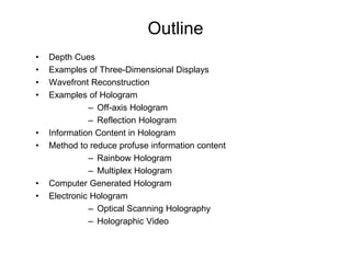
Download as PDF, PPTX

![Depth Cues
• Visual depth sense is often taken for granted until we
encounter the problem that can be solved if depth cues
are present
• Depth Cues can be grouped into two major categories [1]:
1.Psychological (Pictorial) Depth Cues: depth cues
influenced by the mental and prior knowledge of the
observer
2.Physiological Depth Cues: depth cues related to the
physiology of our eyes](https://image.slidesharecdn.com/oippres2001a-130319114355-phpapp01/85/Brief-survey-on-Three-Dimensional-Displays-3-320.jpg)
![Psychological Depth Cues
• Retinal Image Size:
different image size
appearance on
retina
• Aerial Perspective
• Linear Perspective
Figure taken from Ref.[1]](https://image.slidesharecdn.com/oippres2001a-130319114355-phpapp01/85/Brief-survey-on-Three-Dimensional-Displays-4-320.jpg)
![Psychological Depth Cues(Cont’d)
• Occlusion
• Shading
Figures taken from Ref.[1]](https://image.slidesharecdn.com/oippres2001a-130319114355-phpapp01/85/Brief-survey-on-Three-Dimensional-Displays-5-320.jpg)
![Psychological Depth Cues(Cont’d)
• Texture Gradient
Figure taken from Ref.[1]](https://image.slidesharecdn.com/oippres2001a-130319114355-phpapp01/85/Brief-survey-on-Three-Dimensional-Displays-6-320.jpg)
![Physiological Depth Cues
• Accommodation:
Change of eye
muscular tension to
adjust the focal length
• Convergence: eyes
ability to fixate a point
on the object
dα PO
= 2
da a
P0 = two pupil separation
a = object distance
Figure taken from Ref.[1]](https://image.slidesharecdn.com/oippres2001a-130319114355-phpapp01/85/Brief-survey-on-Three-Dimensional-Displays-7-320.jpg)
![Physiological Depth Cues (Cont’d)
• Binocular Disparity/Stereospsis
Dαθ
2
∆D ≅
PO
Figure taken from Ref.[1]
• Motion Parallax: different angular velocity of
object at different depths the observer](https://image.slidesharecdn.com/oippres2001a-130319114355-phpapp01/85/Brief-survey-on-Three-Dimensional-Displays-8-320.jpg)
![Example of Three-Dimensional Displays
• Integral Photography: using lenslet array to sample
the object
Figures taken from Refs.[1,8]](https://image.slidesharecdn.com/oippres2001a-130319114355-phpapp01/85/Brief-survey-on-Three-Dimensional-Displays-9-320.jpg)
![Example of Three-Dimensional Displays(Cont’d)
• Lenticular Sheet
x Figures taken from Ref.[1,2]
θ=
f](https://image.slidesharecdn.com/oippres2001a-130319114355-phpapp01/85/Brief-survey-on-Three-Dimensional-Displays-10-320.jpg)
![Example of Three-Dimensional Displays(Cont’d)
• Parallax Barrier
Figures taken from Refs.[1,2]
viewing distance = .25 m, p < .08 mm → for slit width
1/10 of pitch = 8 µm or only 15 x λvisible](https://image.slidesharecdn.com/oippres2001a-130319114355-phpapp01/85/Brief-survey-on-Three-Dimensional-Displays-11-320.jpg)
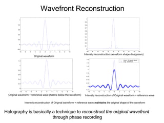
![Three mechanisms of eyes in responding
the incoming wavefront [12,26]
1. Modifies and the focus the wavefront to retina
→Accommodation
2. Sample the wavefront from two slightly different positions and
interpreted as different position in two visual field
→Convergence and Stereopsis
3. Moving observer samples the wavefront from different
positions and object’s position in visual field changes as the
result of observer’s motion
→Motion Parallax
To present all 4 physiological depth cues
Provide or reconstruct the original object’s wavefront](https://image.slidesharecdn.com/oippres2001a-130319114355-phpapp01/85/Brief-survey-on-Three-Dimensional-Displays-12-320.jpg)
![Examples of Hologram
• Transmission Hologram
• Reflection hologram
Figures taken from Refs.[6,8]](https://image.slidesharecdn.com/oippres2001a-130319114355-phpapp01/85/Brief-survey-on-Three-Dimensional-Displays-14-320.jpg)
![Information Content in a Hologram [23,28]
• Grating equation λf h = sin θ
– fh highest frequency comp. of object
• Required sampling freq sin θ
fs = 2 fh = 2
– fs = sampling frequency λ
• N= Number of sampling (in horizontal direction) 2d sin θ
N = df s =
– d = width of hologram in horizontal direction λ
• Nt= Total number of sample in both horizontal and vertical direction
– w=width of hologram in vertical direction 4dw sin θ
Nt =
λ2
• 100 x 100 mm2, 30° view angle →2.5x10¹⁰ samples/frame
• Real time hologram of 60 frames per second requires
→1.2x1012 bit/sec (fastest conventional display rate 2 Gbits/s) [23,28]](https://image.slidesharecdn.com/oippres2001a-130319114355-phpapp01/85/Brief-survey-on-Three-Dimensional-Displays-15-320.jpg)
![Holographic Information Reduction Method
• Rainbow Hologram
horizontal slit is to remove vertical parallax
→reduce information content Figures taken from Ref.[8]](https://image.slidesharecdn.com/oippres2001a-130319114355-phpapp01/85/Brief-survey-on-Three-Dimensional-Displays-16-320.jpg)
![Holographic Information Reduction Method (Cont’d)
• Multiplex Hologram (Holographic Stereogram)
– Proposed by De Bitteto
Figures taken from Ref.[8]](https://image.slidesharecdn.com/oippres2001a-130319114355-phpapp01/85/Brief-survey-on-Three-Dimensional-Displays-17-320.jpg)
![Holographic Stereogram (Cont’d)
• Cross Hologram
Figures taken from Ref.[3,4,6]
→both hologram exhibit no vertical parallax](https://image.slidesharecdn.com/oippres2001a-130319114355-phpapp01/85/Brief-survey-on-Three-Dimensional-Displays-18-320.jpg)
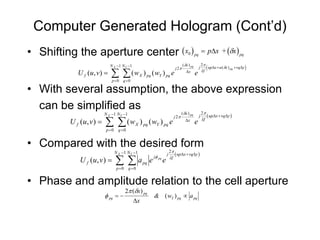
![Computer Generated Hologram
• Binary Detour Phase Method: to create Fourier
Hologram
– Final image must be in the form of
N X −1 N Y −1 2π
( up∆x + vq∆y )
∑ ∑a
j
jφ pq λf
U f ( u, v ) = pq e e
p=0 q =0
– Cell aperture transmittance
x − x0 y − y0
t A ( x , y ) = rect
w X wY
– Inclined plane wave illumination
Figures taken from Ref.[4]
U p = e − j 2παx](https://image.slidesharecdn.com/oippres2001a-130319114355-phpapp01/85/Brief-survey-on-Three-Dimensional-Displays-19-320.jpg)
![Computer Generated Hologram (Cont’d)
• After illumination
− j 2 παx x − x0 y − y0
U t ( x, y) = e rect
wx
w
y
• At Fourier Plane
2π
w w w ( u + λfα ) w v j [ ( u + fλα ) x0 + vy0 ]
U f (u, v ) = X Y sin c X sin c Y e λf
λf λf λf
• After some assumptions, simplifications and
setting the offset ( x ) = p∆x & ( y ) = q∆y 0 pq 0 pq
N X −1 N Y −1 2π
( up∆x + vq∆y )
∑ ∑ (w
j
U f ( u, v ) = X ) pq ( wY ) pq e j 2πp e λf
p=0 q =0](https://image.slidesharecdn.com/oippres2001a-130319114355-phpapp01/85/Brief-survey-on-Three-Dimensional-Displays-20-320.jpg)
![Computer Generated Hologram (Cont’d)
Figures taken from Ref.[4]](https://image.slidesharecdn.com/oippres2001a-130319114355-phpapp01/85/Brief-survey-on-Three-Dimensional-Displays-22-320.jpg)
![Electronic Holography
• Using dynamic electronically-controlled optical modulator
1. Optical Scanning Holography: scanning TDFZP to obtain the
scanned holographic pattern of the object
Application in fluorescence microscopy: for image region 2 x 2
mm2, the system can reveal lateral and axial resolution of 7.7
and 200 µm, respectively
Figures taken from Ref.[5,16]](https://image.slidesharecdn.com/oippres2001a-130319114355-phpapp01/85/Brief-survey-on-Three-Dimensional-Displays-23-320.jpg)
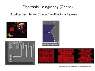
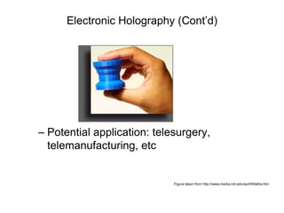
![Electronic Holography (Cont’d)
– Holographic video (Media Lab MIT)
• inspired by binary detour phase, holographic
stereogram and rainbow hologram
• using AOM to diffract light into desired point in
volume space
• fringe calculation is similar to computer
graphics
Figures taken from Ref.[29]](https://image.slidesharecdn.com/oippres2001a-130319114355-phpapp01/85/Brief-survey-on-Three-Dimensional-Displays-24-320.jpg)
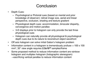


This document provides an overview of three-dimensional displays, from physiological depth cues to electronic holograms. It discusses depth cues our eyes use to perceive depth, including psychological cues like occlusion and physiological cues like binocular disparity. Examples of 3D displays that provide some depth cues, like lenticular sheets, are described. The document also covers holograms, including how they can provide all depth cues by reconstructing the original wavefront. It discusses challenges like the large amount of information in holograms and methods to reduce it, like rainbow and multiplex holograms. Computer generated and electronic holograms using dynamic modulators are also summarized.