Download to read offline
![EEG DATASETS
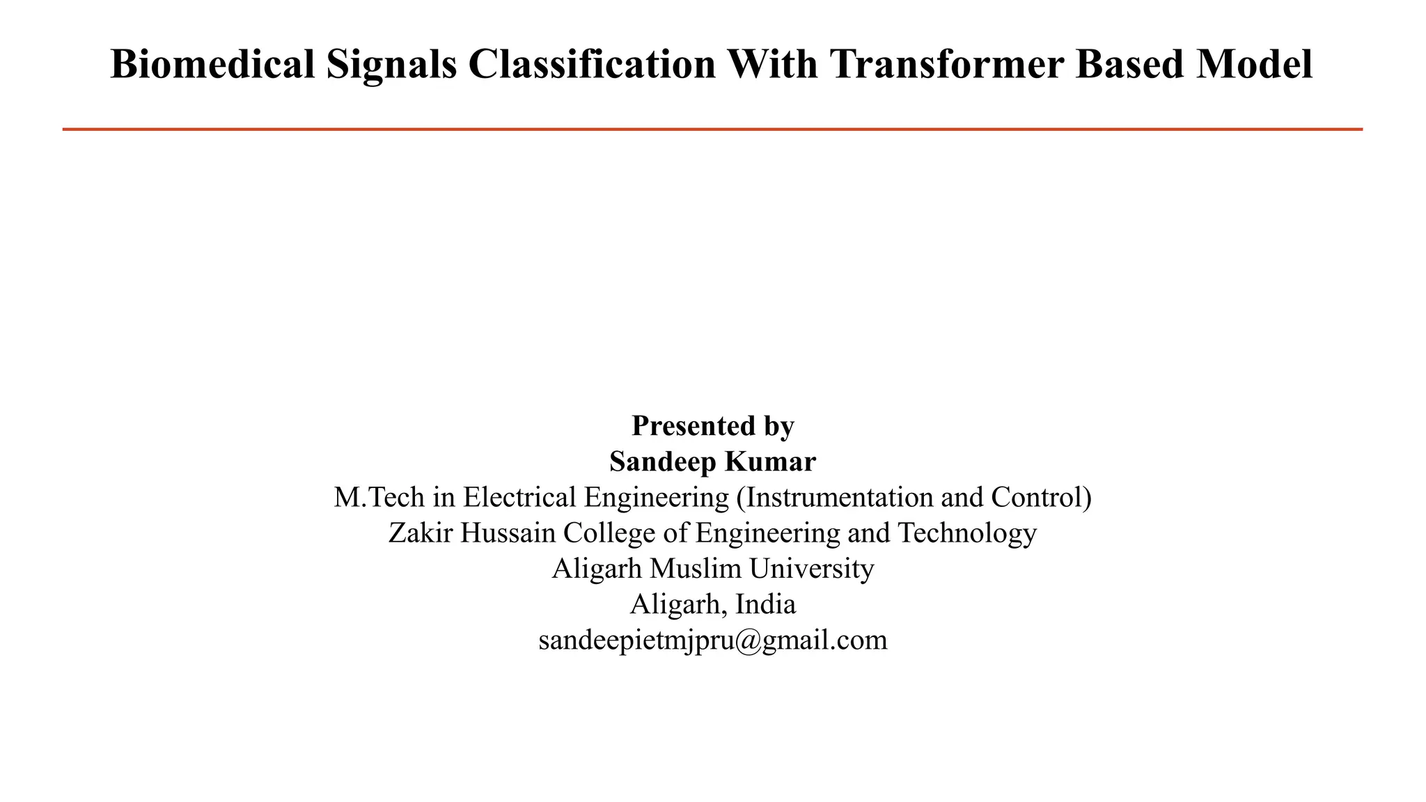
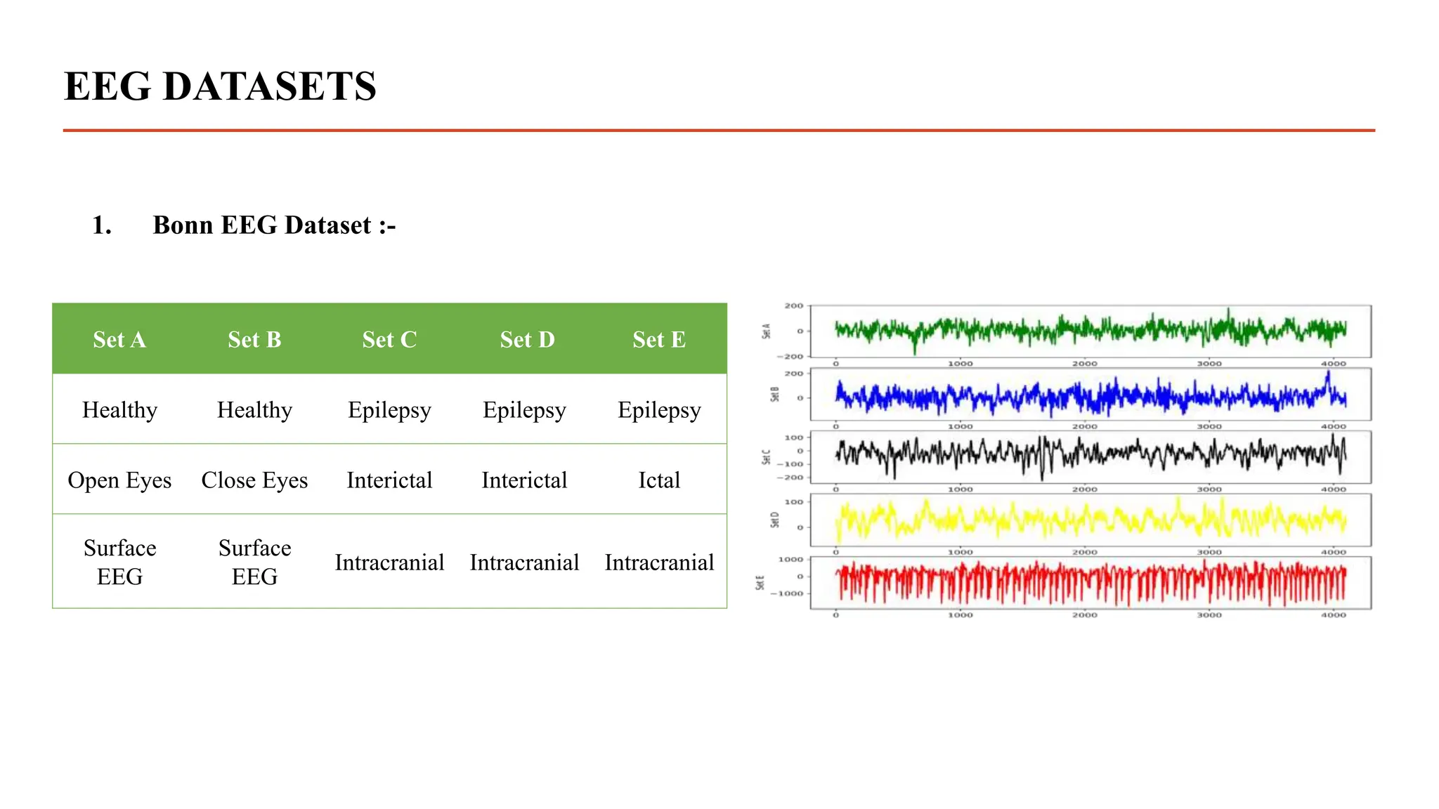
1. Bonn EEG Dataset :-
This EEG datasets[2] come from Bonn University in Germany, which is also the location of the database that is
publicly accessible to the general public.
a) Every class contains 100 text files which represent 100 channels.
b) Database includes five distinct classes, from class A to class E
c) Each channels contains 4097 samples
d) Sampling frequency = 173.6 Hz
e) Time duration of the signals = 4097/173.6 = 23.6 sec](https://image.slidesharecdn.com/dissertationpresentation-231010164640-21e345d6/75/Biomedical-Signals-Classification-With-Transformer-Based-Model-pptx-5-2048.jpg)
![EEG DATASETS
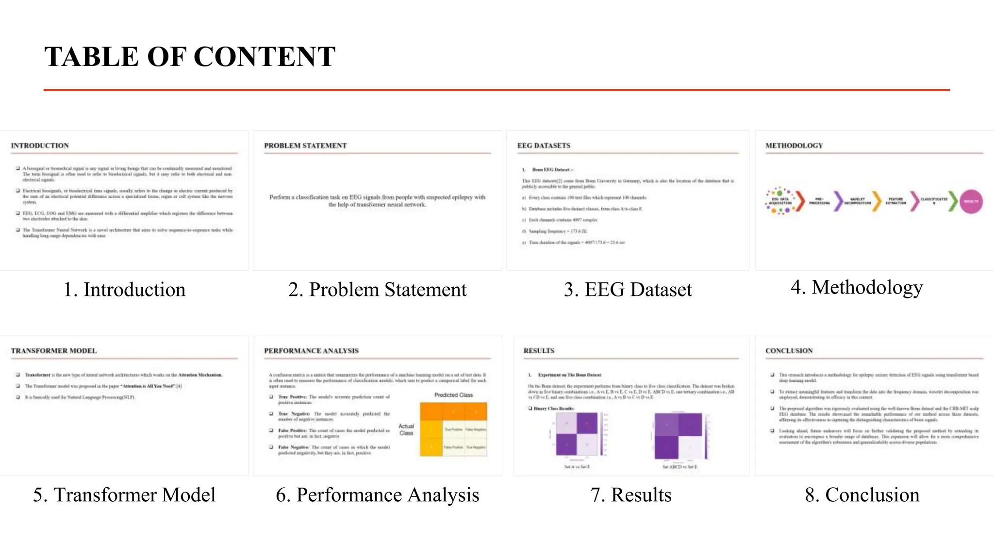
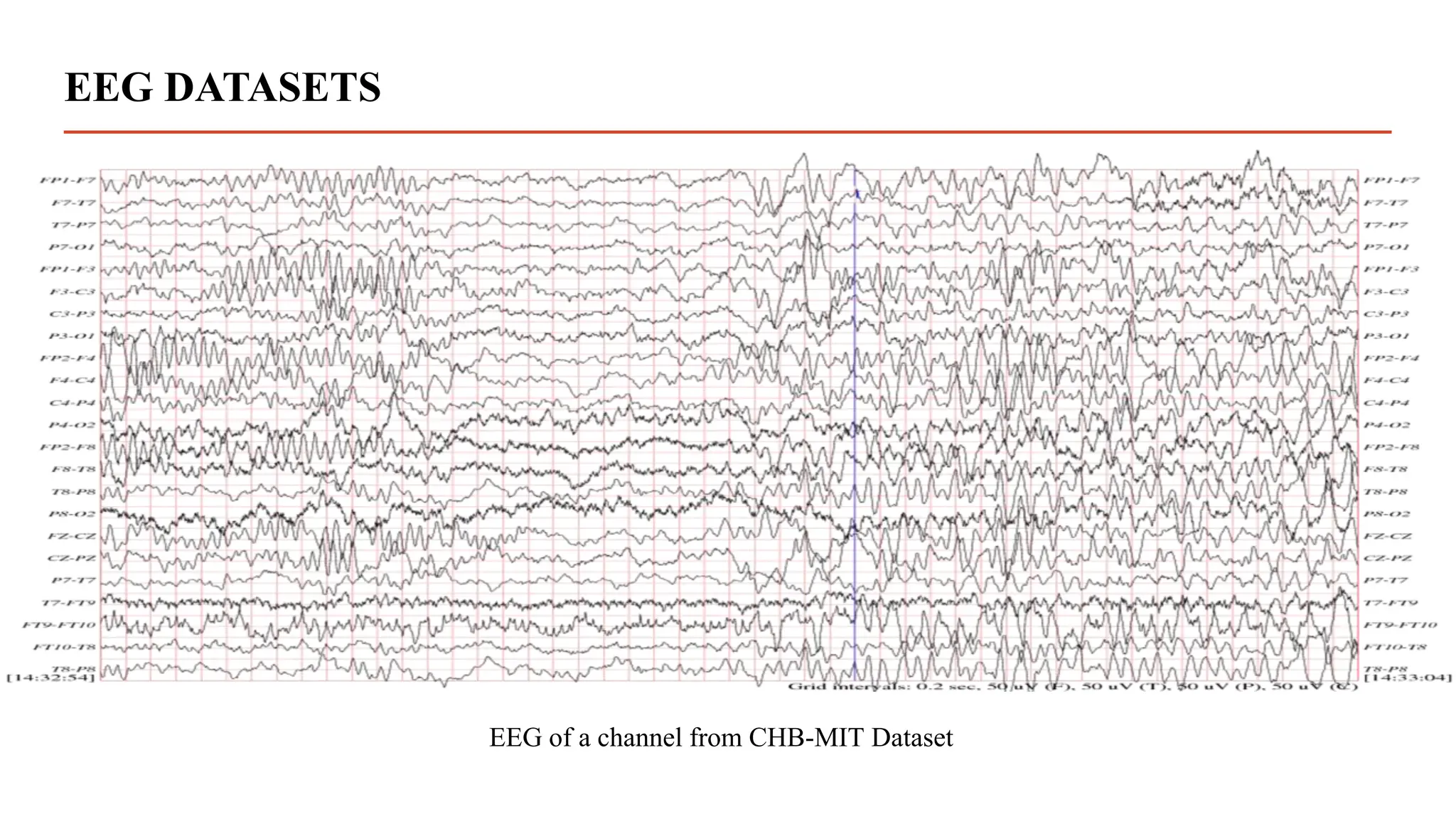
2. CHB-MIT EEG Dataset :-
This database[3], collected at the Children’s Hospital Boston, consists of EEG recordings from pediatric subjects
with intractable seizures. Subjects were monitored for up to several days following withdrawal of anti-seizure
medication in order to characterize their seizures and assess their candidacy for surgical intervention.
a) Recordings, grouped into 23 cases, were collected from 22 subjects (5 males, ages 3–22; and 17 females, ages
1.5–19).
b) All signals were sampled at 256 samples per second (Hz) with 16-bit resolution.](https://image.slidesharecdn.com/dissertationpresentation-231010164640-21e345d6/75/Biomedical-Signals-Classification-With-Transformer-Based-Model-pptx-7-2048.jpg)
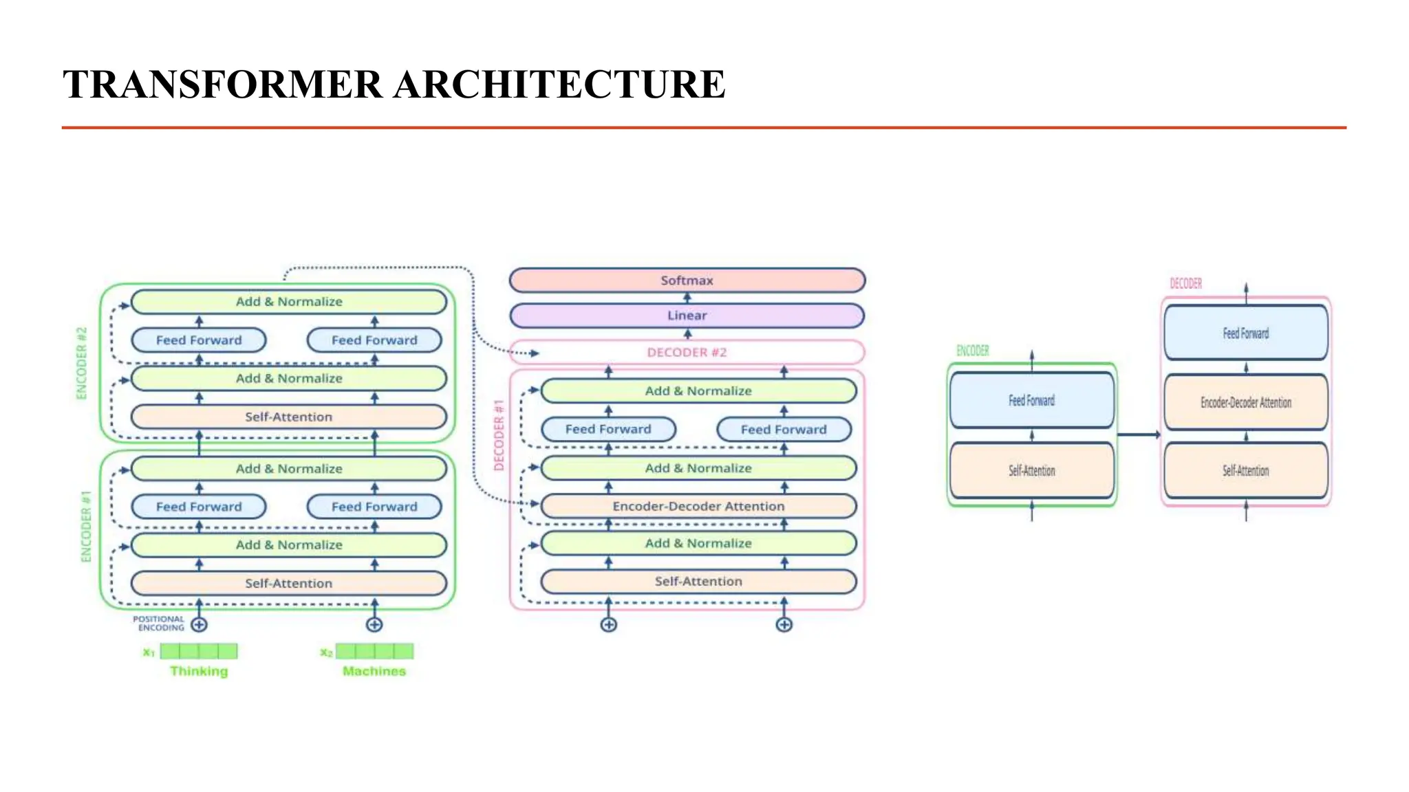
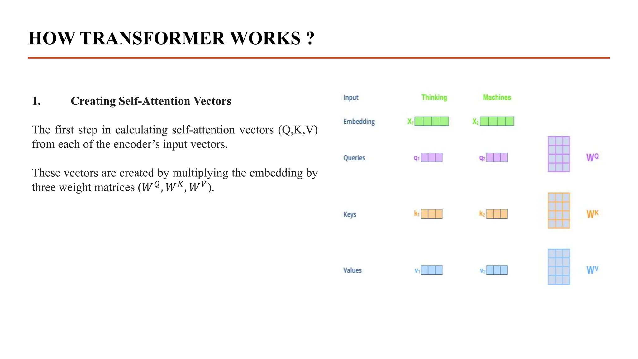
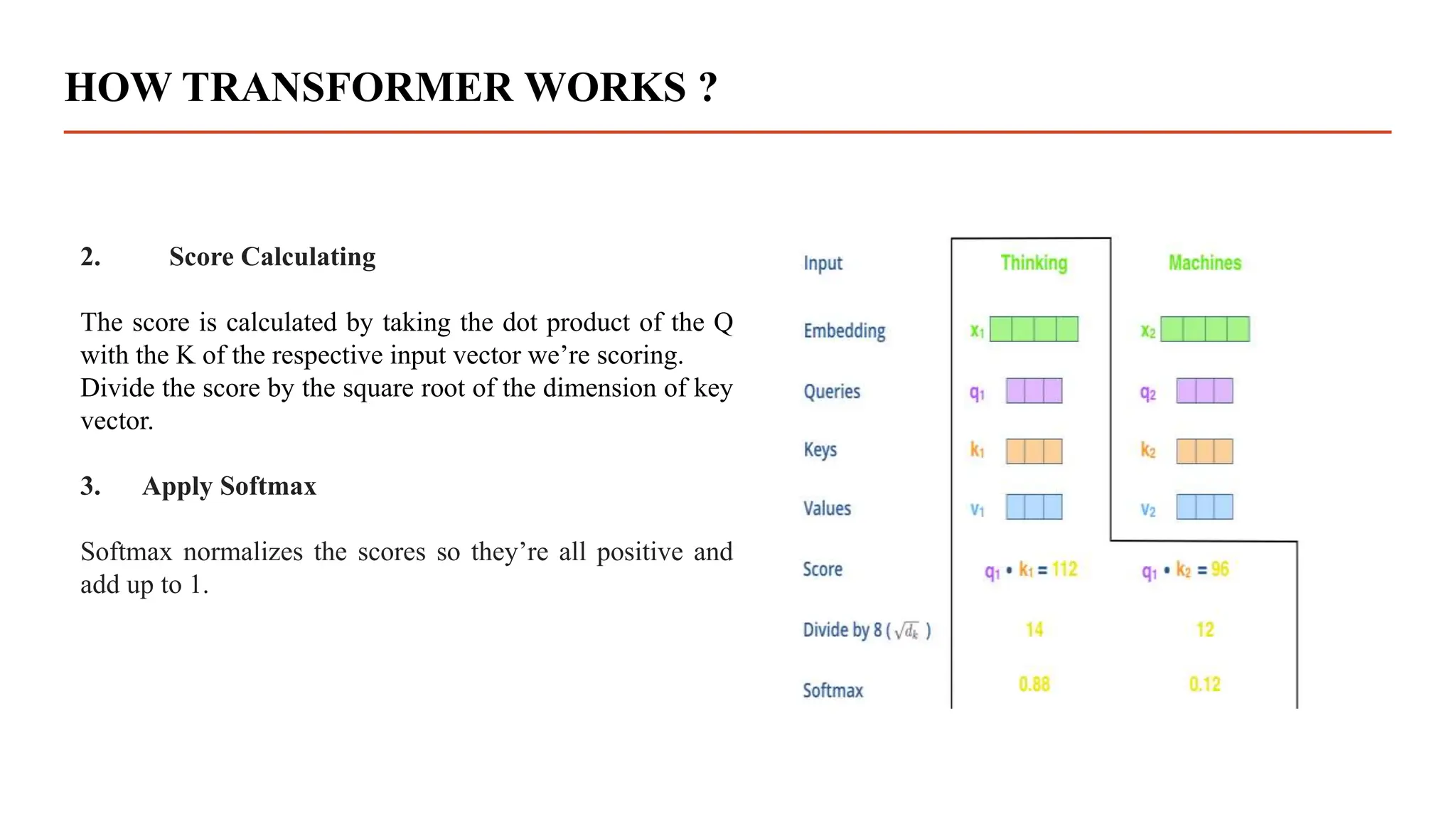
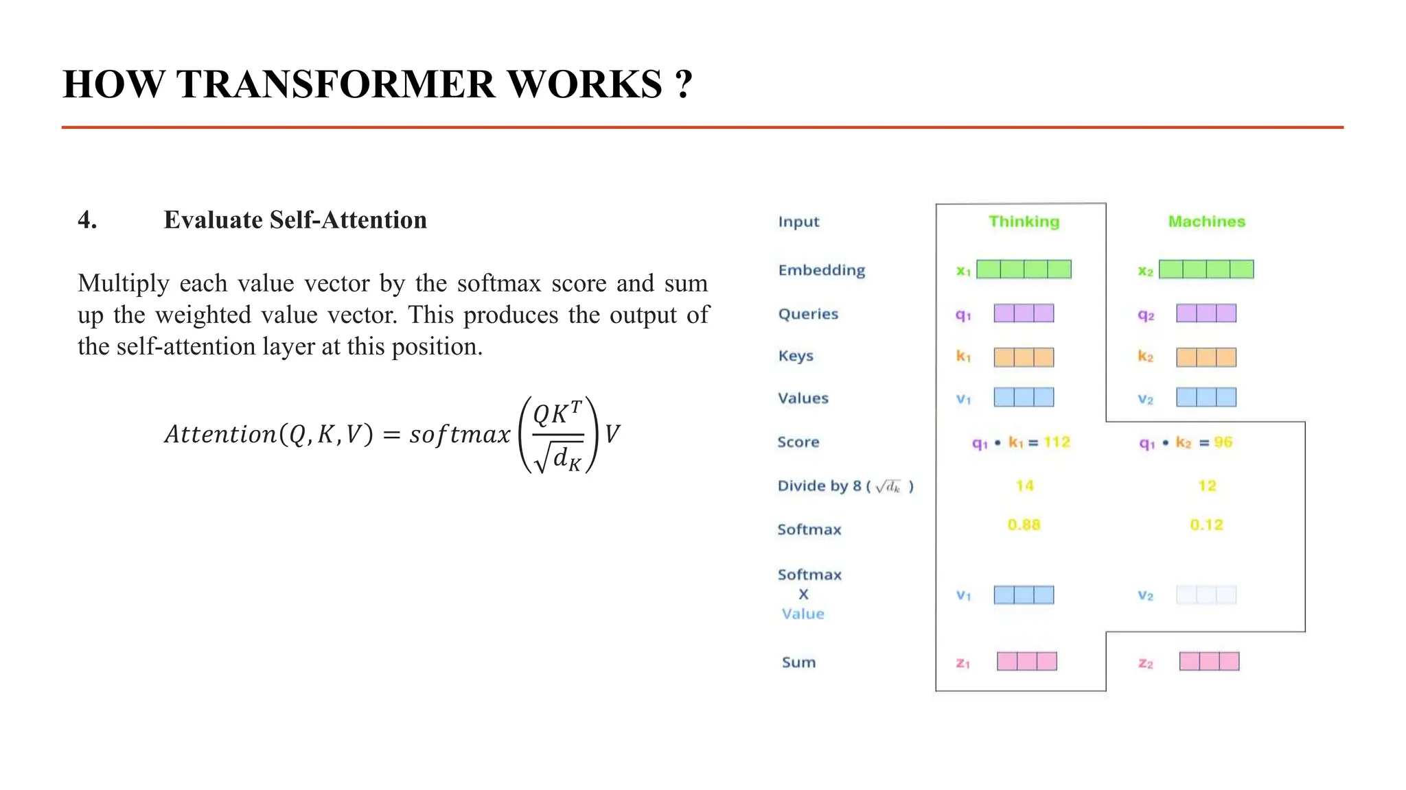
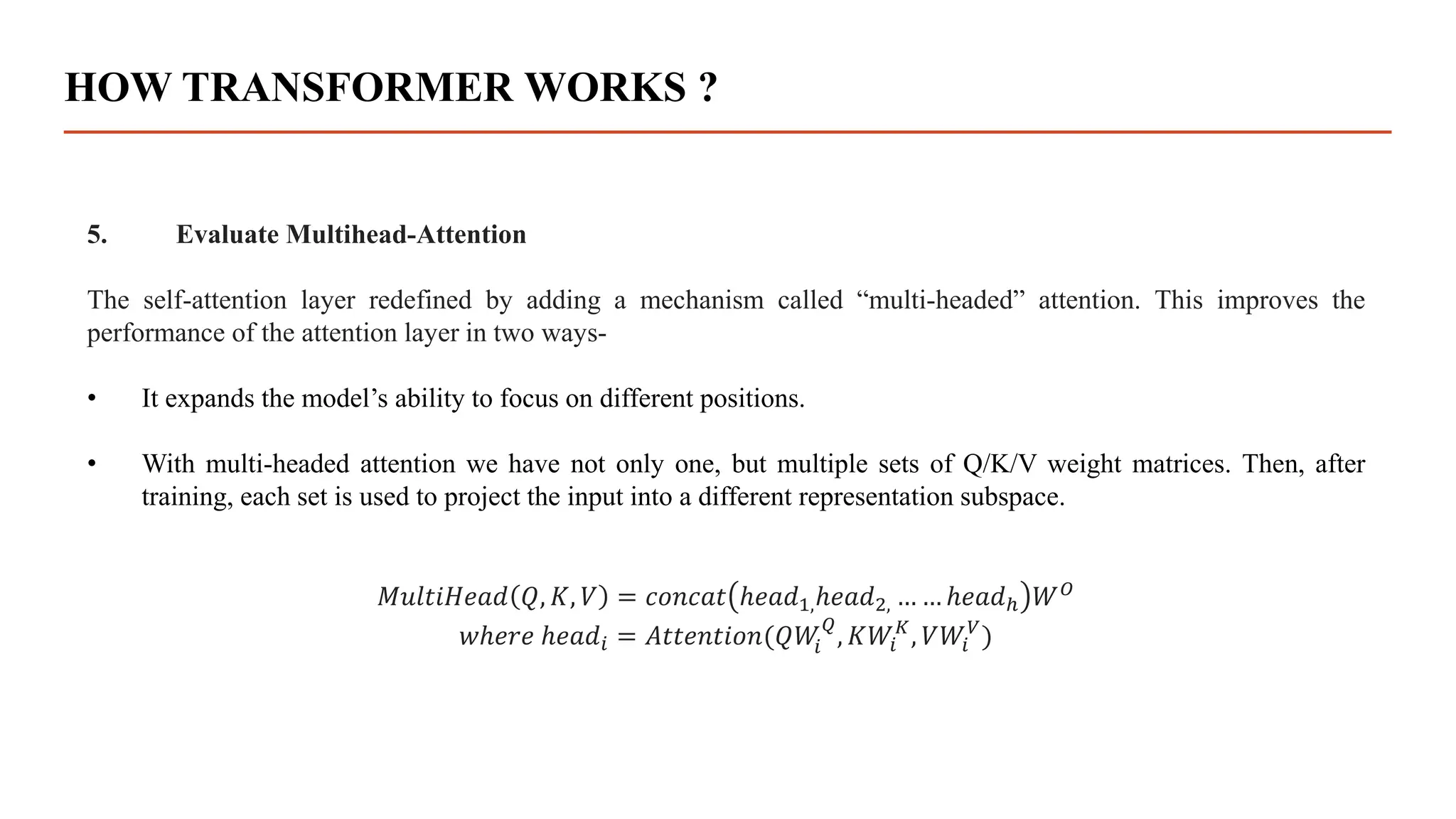
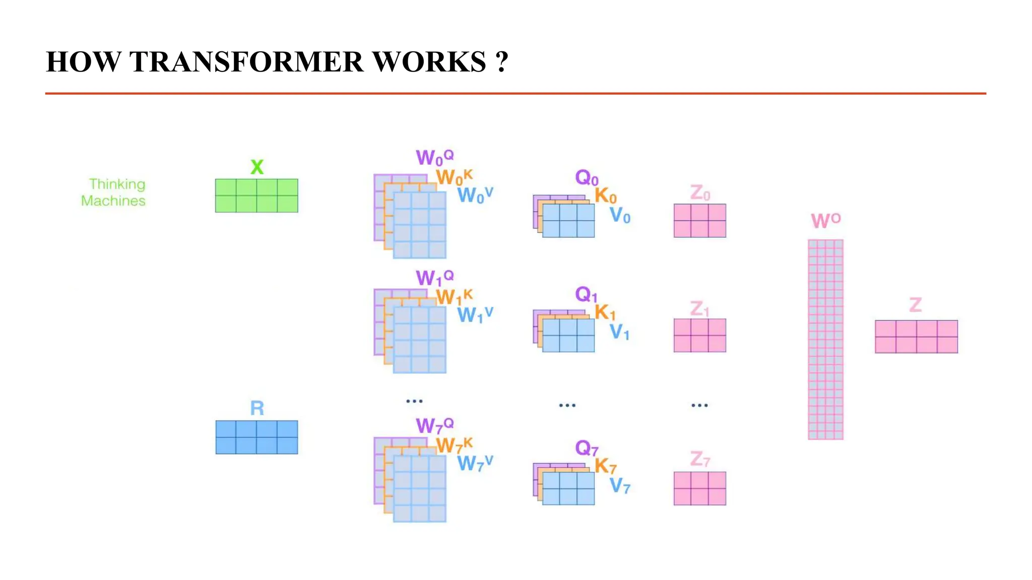
![TRANSFORMER MODEL
Transformer is the new type of neural network architectures which works on the Attention Mechanism.
The Transformer model was proposed in the paper “Attention is All You Need”.[4]
It is basically used for Natural Language Processing(NLP).](https://image.slidesharecdn.com/dissertationpresentation-231010164640-21e345d6/75/Biomedical-Signals-Classification-With-Transformer-Based-Model-pptx-17-2048.jpg)

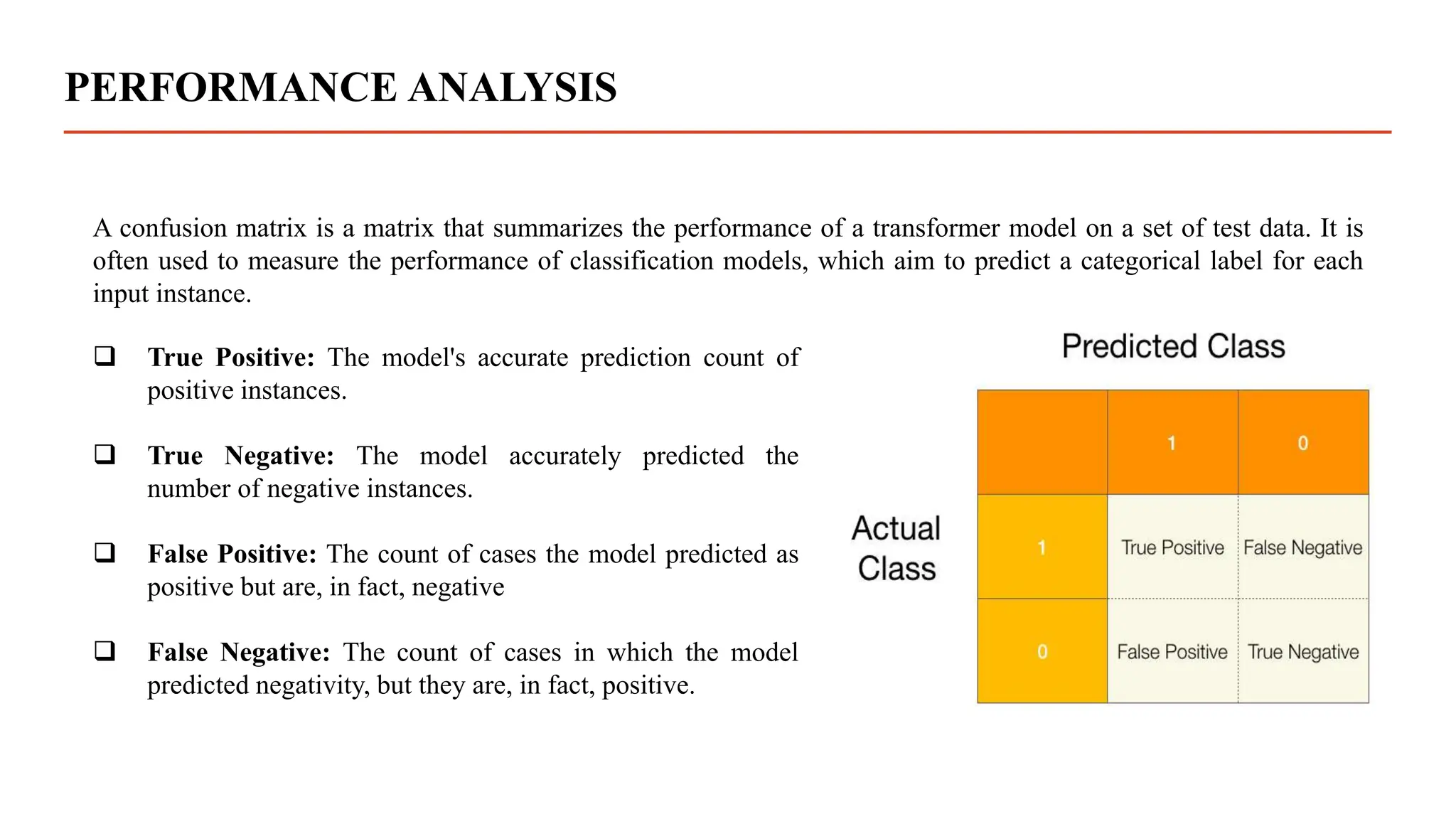
![RESULTS COMPARISION
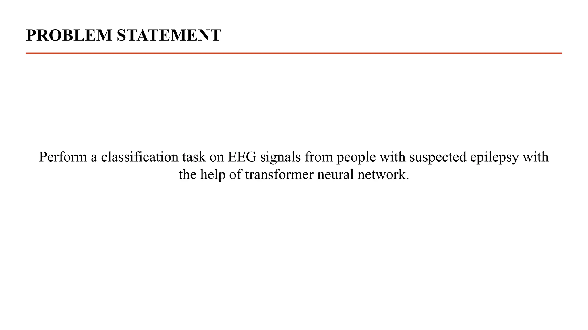
Author/Year Methodology Accuracy
Guo et al.[12]
2010
Multiple layer Perceptron 95%
Tawfik et al.[13]
2016
Support Vector Machine 97%
Wani et al.[14]
2019
Artificial Neural Network
(ANN)
95%
Chowdhury et al.[15]
2019
Convolution Neural Network 99%
Chua et al.[16]
2011
Gaussian Based Classification 93%
Proposed Work Transformer Neural Network 97%](https://image.slidesharecdn.com/dissertationpresentation-231010164640-21e345d6/75/Biomedical-Signals-Classification-With-Transformer-Based-Model-pptx-34-2048.jpg)
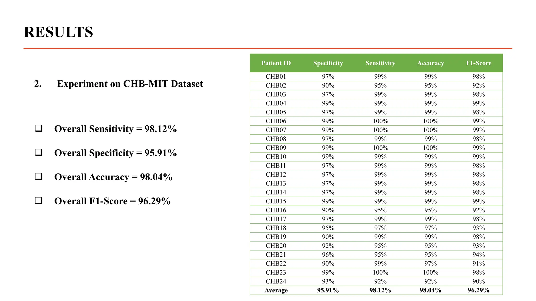


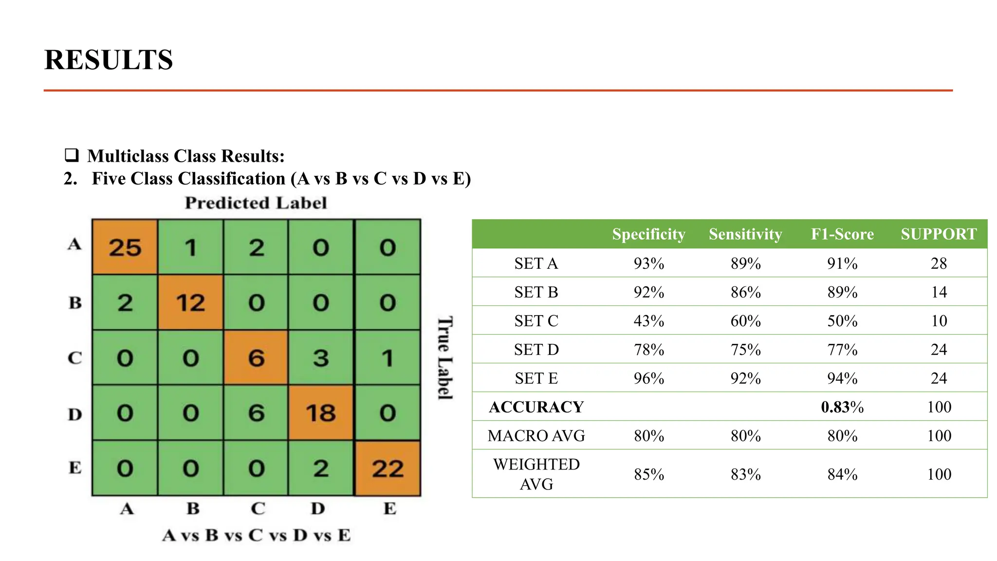
The document summarizes research using a transformer model to classify biomedical signals, specifically EEG signals. Key points: - A transformer model was used to classify EEG signals from epilepsy patients using statistical features extracted from wavelet decompositions of the signals. - The model was tested on the Bonn and CHB-MIT EEG datasets, achieving accuracy above 97% on binary, tertiary and 5-class problems from the Bonn data and above 95% accuracy for individual patients in the CHB-MIT data. - The transformer model outperformed previous methods like MLP, SVM, ANN and CNN in classifying the EEG signals, demonstrating its effectiveness for biomedical signal classification tasks.


![[Research] Detection of MCI using EEG Relative Power + DNN](https://cdn.slidesharecdn.com/ss_thumbnails/20180619a-gisteegaddiagnosisdkimconference-180622113717-thumbnail.jpg?width=640&height=640&fit=bounds)


