Servo systems

1. Servo Systems
In the servo system we want the output to follow the input for a single-input single-
output system. Moreover, for multi-inputs multi-outputs system we want each output to
follow its corresponding input and thus, we assume that we have the same number of
inputs as that of the outputs. To achieve that, we need to add integrators in the path of
the error (inputs r(k) – outputs y(k)). In what follows, we shall show how to design a
servo system using the concept of state feedback for controllable and observable
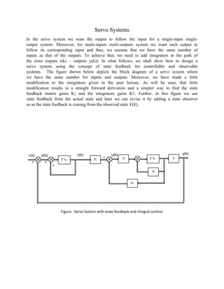
systems. The figure shown below depicts the block diagram of a servo system where
we have the same number for inputs and outputs. Moreover, we have made a little
modification to the integrators given in the past lecture. As will be seen, that little
modification results in a straight forward derivation and a simpler way to find the state
feedback matrix gains K2 and the integrators gains K1. Further, in this figure we use
state feedback from the actual state and later we can revise it by adding a state observer
so as the state feedback is coming from the observed state 𝑥̂(𝑘).
Z-1In
G
C
K2
Figure: Servo System with state feedback and integral control.
r(k) u(k)v(k)
Z-1Im
H
+
+
+
+K1
- -
e(k) y(k)

2. The plant state equation and output equation are
x(k+1) = G x(k) + H u(k) (1)
y(k) = C x(k) (2)
where, number of inputs r = number of outputs m
G is nxn matrix, H is nxm matrix and C is mxn matrix
From this figure we get that
u(k) = K1 v(k) - K2 x(k) (3)
where K2 is the state feedback gain matrix and K1 is the forward loop integrator gains.
The inputs to the integrators e(k) and the outputs v(k) are related by
v(k+1) = e(k) + v(k)
= v(k) + r(k) – y(k) (4)
= v(k) – C x(k) + r(k) (5)
In what follows we shall show how to choose the gain matrices K1 and K2 so as to
locate the combined (n+m) closed loop poles of the system shown in Figure to desired
locations. Note, the combined system shown in Fig. has n state of the original system
eqn. (1) as well as an additional m state introduced due the added m integrators. Next,
let us write the state equation of the combined state x(k) and v(k) in order to use it for
pole placement.
Substituting for the expression of u(k) of eqn. (3) into eqn. (1), we get
x(k+1) = G x(k) – H K2 x(k) + H K1 v(k) (6)
and from (5), we have
v(k+1) = v(k) – C x(k) + r(k)
The equation of the combined state of the servo system, x(k) and v(k) in matrix form
will be
[
𝑥(𝑘 + 1)
𝑣(𝑘 + 1)
]= [
𝐺 − 𝐻 𝐾2 𝐻 𝐾 1
−C 𝐼 𝑚
] [
𝑥(𝑘)
𝑣(𝑘)
] + [
0
𝐼 𝑚
] r(k) (7)

3. y(k) = [ C : 0 𝑚 ] [
𝑥(𝑘)
𝑣(𝑘)
] (8)
This is the state equation of the servo system shown in Fig. and it remains to select the
state feedback matrix gain K2 of dimension (mxn) and the integrator gains matrix K1 of
dimension (mxm) so as to locate the (n+m) closed loop poles to the inside of the unit
circle. Im stands for the identity matrix of dimension mxm. At steady state
x(k+1) = x(k) = xss
u(k+1) = u(k) = uss
v(k+1) = v(k) = vss
and y(k+1) = y(k) = yss
Thus, it follows from eqn. (4)
vss = vss + r - yss
and hence the steady state value of the outputs will equal the corresponding input for
unit step inputs. We can get the steady state of x(k) and v(k) from eqn. (7).
To find the gain matrices K1 and K2 , let us rewrite eqn. (7) in the form
[
𝑥(𝑘 + 1)
𝑣(𝑘 + 1)
]=[
𝐺 0
−C 𝐼 𝑚
] [
𝑥(𝑘)
𝑣(𝑘)
] + [
0
𝐼 𝑚
] r(k) - [
𝐻 𝐾2 −𝐻𝐾1
0 0
] [
𝑥(𝑘)
𝑣(𝑘)
] (9)
= [
𝐺 0
−C 𝐼 𝑚
] [
𝑥(𝑘)
𝑣(𝑘)
] + [
0
𝐼 𝑚
] r(k) – [
𝐻
0
] [𝐾2 −𝐾1] [
𝑥(𝑘)
𝑣(𝑘)
] (10)
The last term in eqn. (10) represents the combined state feedback gain matrix
[𝐾2 −𝐾1]. We can write equation (10) in the form
𝑥 𝑎(𝑘 + 1) = 𝐺 𝑎 𝑥 𝑎(𝑘) − 𝐻 𝑎 𝐾𝑎 𝑥 𝑎(𝑘) + [
0
𝐼 𝑚
] r(k), and 𝑥 𝑎(𝑘) = [
𝑥(𝑘)
𝑣(𝑘)
] (11)
where 𝐺 𝑎 = [
𝐺 0
−C 𝐼 𝑚
], 𝐻 𝑎 = [
𝐻
0
] and 𝐾𝑎 = [𝐾2 −𝐾1] (12)
and 0 represents a zero matrix with the appropriate dimension so as to make the 𝐺 𝑎
matrix to be (n+m)x(n+m) square matrix while the 𝐻 𝑎 is of dimension mx(n+m).

4. To summarize what we have done, we find the integrators gains K1 and the state
feedback gain matrix K2 so as to locate the (n+m) closed loop poles through the
following steps:
1- Construct the matrices 𝐺 𝑎 and 𝐻 𝑎 of the augmented system as
𝐺 𝑎 = [
𝐺 0
−C 𝐼 𝑚
], 𝐻 𝑎 = [
𝐻
0
]
2- Find the state feedback gain matrix 𝐾𝑎 corresponding to 𝐺 𝑎 and 𝐻 𝑎 .
3- Determine the state feedback gain matrix 𝐾2 the integrators gain matrix 𝐾1 from
eqn. (12) 𝐾𝑎 = [𝐾2 −𝐾1]
It worth mentioning that the pair (Ga , Ha) is controllable.
The following example will illustrate these steps.
Example. Given the system described by
𝑌(𝑧)
𝑋(𝑧)
=
𝑧−2+0.5 𝑧−3
1− 𝑧−1+0.01 𝑧−2+0.12 𝑧−3
Determine the integral gain constant K1 and the state feedback gain matrix K2 so as to locate the
closed loop poles at z1,2 = 0.3 + 0.4 j and z3,4= 0.
Solution:- The standard controllable form representation of the transfer function is
𝑥(𝑘 + 1) = [
0 1 0
0 0 1
−0.12 −0.01 1
] 𝑥(𝑘) + [
0
0
1
] 𝑢(𝑘), 𝑦(𝑘) = [0.5 1 0]𝑥(𝑘)
Where n = 3 and m =1
The servo system matrices G^
and H^
are given by
𝐺 𝑎 = [
𝐺 0
−C 𝐼 𝑚
] = [
0 1 0 0
0 0 1 0
−0.12 −0.01 1 0
−0.5 −1 0 1
] and 𝐻 𝑎 = [
𝐻
0
] = [
0
0
1
0
]
The closed loop characteristic equation of the designed system is given by

5. Φ(z) = z2
(z2
-0.6 z +0.25)
The controllability matrix of the pair (Ga, Ha
^
) = CONA = [
0 0 1 1
0 1 1 0.99
1 1 0.99 0.86
0 0 −1 −2.5
]
The inverse of the controllability matrix is given by
CONA-1
= [
−0.07 −1 1 −0.08
−1.0067 1 0 −0.0067
1.6667 0 0 0.6667
−0.6667 0 0 −0.6667
] ➔ 𝑓4= [−0.6667 0 0 −0.6667]
Note, we could deduce 𝑓4 from 𝑓4 ∗ 𝐶𝑂𝑁́ = [0 0 0 1]
Therefore, the inverse of the transformation to the standard controllable form is given by
Pa
-1
=
[
𝑓4
𝑓4 𝐺 𝑎
𝑓4 𝐺 𝑎
2
𝑓4 𝐺 𝑎
3
]
= [
−0.6667 0 0 −0.6667
0.3333 0 0 −0.6667
0.3333 1 0 −0.6667
0.3333 1 1 −0.6667
] and Pa = [
−1 1 0 0
0 −1 1 0
0 0 −1 1
−0.5 −1 0 0
]
And 𝐺 𝑎
^
= 𝑃𝑎
−1
𝐺 𝑎 𝑃𝑎 = [
0 1 0 0
0 0 1 0
0 0 0 1
0.12 −0.11 −1.01 2
] , 𝐻 𝑎
^
= [
0
0
0
1
]
Therefore Ka = [(∝4− 𝑎4) (∝3− 𝑎3) (∝2− 𝑎2) (∝1− 𝑎1)] 𝑃𝑎
−1
Ka = [ 0.12 -0.11 (0.25-1.01) (-0.6+2)] = [
−0.6667 0 0 −0.6667
0.3333 0 0 −0.6667
0.3333 1 0 −0.6667
0.3333 1 1 −0.6667
]
= [0.0966 0.64 1.4 -0.433]
K2 = [ 0.0966 0.64 1.4 ] and K1 = 0.433
To find the step response of this system, we have to use the augmented state equation

6. [
𝑥(𝑘 + 1)
𝑣(𝑘 + 1)
] = [
𝐺 − 𝐻 𝐾2 𝐻 𝐾 1
−C 𝐼 𝑚
] [
𝑥(𝑘)
𝑣(𝑘)
] + [
0
𝐼 𝑚
] r(k)
and the output equation
y(k) = [ C : 0 ] [
𝑥(𝑘)
𝑣(𝑘)
]
Substituting for G, H, C, K1 and K2 , we get
[
𝑥(𝑘 + 1)
𝑣(𝑘 + 1)
] = [
0 1 0 0
0 0 1 0
−0.2167 −0.65 −0.4 0.4333
−0.5 −1 0 1
] [
𝑥(𝑘)
𝑣(𝑘)
] + [
0
0
0
1
] r(k)
y(k) = [0.5 1 0 0] [
𝑥(𝑘)
𝑢(𝑘)
]
Assuming zero initial conditions for all the state, the computed output step response is
y = [ 0 0 0 0.43 0.91 1.087 1.075 1.023 0.995 0.991 0.996 0.9997 1.00086
1.00057 1.00012 0.9999 0.9999 0.99997 1.00 1.00 1.00 ]
Note : you can use the MATLAB eig function to check the eigenvalues (poles) of the servo-
system eig([
0 1 0 0
0 0 1 0
−0.2167 −0.65 −0.4 0.4333
−0.5 −1 0 1
])

7. It is clear from the response that the output reaches within 2% of the value of the step input after
7 samples. The maximum overshoot of the output is 8.7% and the rise time which is the time
required to rise from 10% to 90% of the steady state is 2 samples.
The response of a servo system to a step input is usually as shown in the following figure which
also illustrates the response characteristics.

8. Rise Time Tr — Time it takes for the response to rise from 10% to 90% of the steady-state
response as in MATLAB, however, others used the time it takes from the start of the response
until it first reaches the value of the input as in this figure. We use the MATLAB definition.
Settling Time Ts — Time it takes for the error |y(t) - yfinal| between the response y(t) and the
steady-state response yfinal to fall to within 2% of yfinal.
Overshoot — Maximum percentage overshoot, relative to yfinal
Undershoot — Percentage undershoot.
Peak — Peak absolute value of y(t)
Peak Time Tp — Time at which the peak value occurs.
Assuming that the sampling period of this example is 0.1 sec, the characteristics of the
designed servo system as calculated from MATLAB function stepinfo are
RiseTime: 0.1748 SettlingTime: 0.7112
SettlingMin: 0.9099 SettlingMax: 1.0876
Overshoot: 8.7583 Undershoot: 0
Peak: 1.0876 PeakTime: 0.5000