Best Keyword Cover Search

Best Keyword Cover Search
Ke Deng, Xin Li, Jiaheng Lu, and Xiaofang Zhou, Senior Member, IEEE
Abstract—It is common that the objects in a spatial database (e.g., restaurants/hotels) are associated with keyword(s) to indicate their
businesses/services/features. An interesting problem known as Closest Keywords search is to query objects, called keyword cover,
which together cover a set of query keywords and have the minimum inter-objects distance. In recent years, we observe the increasing
availability and importance of keyword rating in object evaluation for the better decision making. This motivates us to investigate a generic
version of Closest Keywords search called Best Keyword Cover which considers inter-objects distance as well as the keyword rating of
objects. The baseline algorithm is inspired by the methods of Closest Keywords search which is based on exhaustively combining objects
from different query keywords to generate candidate keyword covers. When the number of query keywords increases, the performance
of the baseline algorithm drops dramatically as a result of massive candidate keyword covers generated. To attack this drawback, this
work proposes a much more scalable algorithm called keyword nearest neighbor expansion (keyword-NNE). Compared to the baseline
algorithm, keyword-NNE algorithm significantly reduces the number of candidate keyword covers generated. The in-depth analysis and
extensive experiments on real data sets have justified the superiority of our keyword-NNE algorithm.
Index Terms—Spatial database, point of interests, keywords, keyword rating, keyword cover
Ç
1 INTRODUCTION
DRIVEN by mobile computing, location-based services
and wide availability of extensive digital maps and
satellite imagery (e.g., Google Maps and Microsoft Virtual
Earth services), the spatial keywords search problem has
attracted much attention recently [3], [4], [5], [7], [8], [10],
[15], [16], [18].
In a spatial database, each tuple represents a spatial object
which is associated with keyword(s) to indicate the informa-
tion such as its businesses/services/features. Given a set of
query keywords, an essential task of spatial keywords search
is to identify spatial object(s) which are associated with key-
words relevant to a set of query keywords, and have desir-
able spatial relationships (e.g., close to each other and/or
close to a query location). This problem has unique value in
various applications because users’ requirements are often
expressed as multiple keywords. For example, a tourist who
plans to visit a city may have particular shopping, dining
and accommodation needs. It is desirable that all these needs
can be satisfied without long distance traveling.
Due to the remarkable value in practice, several variants
of spatial keyword search problem have been studied. The
works [5], [7], [8], [15] aim to find a number of individual
objects, each of which is close to a query location and the
associated keywords (or called document) are very relevant
to a set of query keywords (or called query document). The
document similarity (e.g., [14]) is applied to measure the rel-
evance between two sets of keywords. Since it is likely none
of individual objects is associated with all query keywords,
this motivates the studies [4], [17], [18] to retrieve multiple
objects, called keyword cover, which together cover (i.e., asso-
ciated with) all query keywords and are close to each other.
This problem is known as m Closest Keywords (mCK) query
in [17], [18]. The problem studied in [4] additionally
requires the retrieved objects close to a query location.
This paper investigates a generic version of mCK query,
called Best Keyword Cover (BKC) query, which considers
inter-objects distance as well as keyword rating. It is moti-
vated by the observation of increasing availability and
importance of keyword rating in decision making. Millions
of businesses/services/features around the world have been
rated by customers through online business review sites
such as Yelp, Citysearch, ZAGAT and Dianping, etc. For
example, a restaurant is rated 65 out of 100 (ZAGAT.com)
and a hotel is rated 3.9 out of 5 (hotels.com). According to
a survey in 2013 conducted by Dimensional Research
(dimensionalresearch.com), an overwhelming 90 percent of
respondents claimed that buying decisions are influenced by
online business review/rating. Due to the consideration of
keyword rating, the solution of BKC query can be very dif-
ferent from that of mCK query. Fig. 1 shows an example.
Suppose the query keywords are “Hotel”, “Restaurant” and
“Bar”. mCK query returns ft2; s2; c2g since it considers the
distance between the returned objects only. BKC query
returns ft1; s1; c1g since the keyword ratings of object are con-
sidered in addition to the inter-objects distance. Compared to
mCK query, BKC query supports more robust object evalua-
tion and thus underpins the better decision making.
This work develops two BKC query processing
algorithms, baseline and keyword-NNE. The baseline algo-
rithm is inspired by the mCK query processing methods
[17], [18]. Both the baseline algorithm and keyword-NNE algo-
rithm are supported by indexing the objects with an R*-tree
like index, called KRR*-tree. In the baseline algorithm, the
K. Deng is with Huawei Noah’s Ark Research Lab, Hong Kong.
E-mail: deng.ke@huawei.com.
X. Li and J. Lu are with the Department of Computer Science, Renmin
University, China. E-mail: {lixin2007, jiahenglu}@ruc.edu.cn.
X. Zhou is with the School of Information Technology and Electrical
Engineering, The University of Queensland, QLD, 4072, Australia, and
the School of Computer Science and Technology, Soochow University,
China. E-mail: zxf@itee.uq.edu.au.
Manuscript received 9 July 2013; revised 27 Apr. 2014; accepted 8 May 2014.
Date of publication 22 May 2014; date of current version 1 Dec. 2014.
Recommended for acceptance by J. Sander.
For information on obtaining reprints of this article, please send e-mail to:
reprints@ieee.org, and reference the Digital Object Identifier below.
Digital Object Identifier no. 10.1109/TKDE.2014.2324897
IEEE TRANSACTIONS ON KNOWLEDGE AND DATA ENGINEERING, VOL. 27, NO. 1, JANUARY 2015 61
1041-4347 ß 2014 IEEE. Personal use is permitted, but republication/redistribution requires IEEE permission.
See http://www.ieee.org/publications_standards/publications/rights/index.html for more information.

idea is to combine nodes in higher hierarchical levels of
KRR*-trees to generate candidate keyword covers. Then,
the most promising candidate is assessed in priority by
combining their child nodes to generate new candidates.
Even though BKC query can be effectively resolved, when
the number of query keywords increases, the performance
drops dramatically as a result of massive candidate key-
word covers generated.
To overcome this critical drawback, we developed much
scalable keyword nearest neighbor expansion (keyword-NNE)
algorithm which applies a different strategy. Keyword-
NNE selects one query keyword as principal query keyword.
The objects associated with the principal query keyword
are principal objects. For each principal object, the local best
solution (known as local best keyword cover ðlbkcÞ) is com-
puted. Among them, the lbkc with the highest evaluation is
the solution of BKC query. Given a principal object, its
lbkc can be identified by simply retrieving a few nearby
and highly rated objects in each non-principal query key-
word (two-four objects in average as illustrated in experi-
ments). Compared to the baseline algorithm, the number
of candidate keyword covers generated in keyword-NNE
algorithm is significantly reduced. The in-depth analysis
reveals that the number of candidate keyword covers fur-
ther processed in keyword-NNE algorithm is optimal, and
each keyword candidate cover processing generates much
less new candidate keyword covers than that in the base-
line algorithm.
In the remainder of this paper, the problem is defined in
Section 2 and the related work is reviewed in Section 3.
Section 4 discusses keyword rating R*-tree. The baseline
algorithm and keyword-NNE algorithm are introduced in
Sections 5 and 6, respectively. Section 7 discusses the situa-
tion of weighted average of keyword ratings. An in-depth
analysis is given in Section 8. Then Section 9 reports the
experimental results. The paper is concluded in Section 10.
2 PRELIMINARY
Given a spatial database, each object may be associated with
one or multiple keywords. Without loss of generality, the
object with multiple keywords are transformed to multiple
objects located at the same location, each with a distinct sin-
gle keyword. So, an object is in the form hid; x; y; keyword;
ratingi where x; y define the location of the object in a two-
dimensional geographical space. No data quality problem
such as misspelling exists in keywords.
Definition 1 (Diameter). Let O be a set of objects fo1; . . . ; ong.
For oi; oj 2 O, distðoi; ojÞ is the euclidean distance between
oi; oj in the two-dimensional geographical space. The diameter
of O is
diamðOÞ ¼ max
oi;oj2O
distðoi; ojÞ: (1)
The score of O is a function with respect to not only the
diameter of O but also the keyword rating of objects in O.
Users may have different interests in keyword rating of
objects. We first discuss the situation that a user expects to
maximize the minimum keyword rating of objects in BKC
query. Then we will discuss another situation in Section 7
that a user expects to maximize the weighted average of
keyword ratings.
The linear interpolation function [5], [16] is used to
obtain the score of O such that the score is a linear interpola-
tion of the individually normalized diameter and the mini-
mum keyword rating of O.
O:score ¼ scoreðA; BÞ
¼ a 1 À
A
max dist

þ ð1 À aÞ
B
max rating
:
A ¼ diamðOÞ:
B ¼ min
o2O
ðo:ratingÞ;
(2)
where B is the minimum keyword rating of objects in O and
að0 a 1Þ is an application specific parameter. If a ¼ 1,
the score of O is solely determined by the diameter of O. In
this case, BKC query is degraded to mCK query. If a ¼ 0,
the score of O only considers the minimum keyword rating
of objects in Q where max dist and max rating are used to
normalize diameter and keyword rating into [0, 1] respec-
tively. max dist is the maximum distance between any two
objects in the spatial database D, and max rating is the max-
imum keyword rating of objects.
Lemma 1. The score is of monotone property.
Proof. Given a set of objects Oi, suppose Oj is a subset of Oi.
The diameter of Oi must be not less than that of Oj, and
the minimum keyword rating of objects in Oi must be
not greater than that of objects in Oj. Therefore,
Oi:score Oj:score. tu
Definition 2 (Keyword Cover). Let T be a set of keywords
fk1; . . . ; kng and O a set of objects fo1; . . . ; ong, O is a key-
word cover of T if one object in O is associated with one and
only one keyword in T.
Definition 3 (Best Keyword Cover Query). Given a spatial
database D and a set of query keywords T, BKC query returns
a keyword cover O of T (O D) such that O:score !
O0
:score for any keyword cover O0
of T (O0
D).
The notations used in this work are summarized in Table 1.
3 RELATED WORK
3.1 Spatial Keyword Search
Recently, the spatial keyword search has received consider-
able attention from research community. Some existing
works focus on retrieving individual objects by specifying
Fig. 1. BKC versus mCK.
62 IEEE TRANSACTIONS ON KNOWLEDGE AND DATA ENGINEERING, VOL. 27, NO. 1, JANUARY 2015

a query consisting of a query location and a set of query
keywords (or known as document in some context). Each
retrieved object is associated with keywords relevant to the
query keywords and is close to the query location [3], [5],
[7], [8], [10], [15], [16]. The similarity between documents
(e.g., [14]) are applied to measure the relevance between
two sets of keywords.
Since it is likely no individual object is associated with
all query keywords, some other works aim to retrieve mul-
tiple objects which together cover all query keywords [4],
[17], [18]. While potentially a large number of object combi-
nations satisfy this requirement, the research problem is
that the retrieved objects must have desirable spatial rela-
tionship. In [4], authors put forward the problem to
retrieve objects which 1) cover all query keywords, 2) have
minimum inter-objects distance and 3) are close to a query
location. The work [17], [18] study a similar problem called
m Closet Keywords (mCK). mCK aims to find objects
which cover all query keywords and have the minimum
inter-objects distance. Since no query location is asked in
mCK, the search space in mCK is not constrained by the
query location. The problem studied in this paper is a
generic version of mCK query by also considering key-
word rating of objects.
3.2 Access Methods
The approaches proposed by Cong et al. [5] and Li et al. [10]
employ a hybrid index that augments nodes in non-leaf
nodes of an R/R*-tree with inverted indexes. The inverted
index at each node refers to a pseudo-document that repre-
sents the keywords under the node. Therefore, in order to
verify if a node is relevant to a set of query keywords, the
inverted index is accessed at each node to evaluate the match-
ing between the query keywords and the pseudo-document
associated with the node.
In [18], bR*-tree was proposed where a bitmap is kept for
each node instead of pseudo-document. Each bit corresponds
to a keyword. If a bit is “1”, it indicates some object(s) under
the node is associated with the corresponding keyword; “0”
otherwise. A bR*-tree example is shown in Fig. 2a where a
non-leaf node N has four child nodes N1, N2, N3, and N4. The
bitmaps of N1; N2; N4 are 111 and the bitmap of N3 is 101. In
specific, the bitmap 101 indicates some objects under N3 are
associated with keyword “hotel” and “restaurant” respec-
tively, and no object under N3 is associated with keyword
“bar”. The bitmap allows to combine nodes to generate candi-
date keyword covers. If a node contains all query keywords,
this node is a candidate keyword cover. If multiple nodes
together cover all query keywords, they constitute a candidate
keyword cover. Suppose the query keywords are 111. When
N is visited, its child node N1; N2; N3; N4 are processed.
N1; N2; N4 are associated with all query keywords and N3 is
associated with two query keywords. The candidate keyword
covers generated are fN1g, fN2g, fN4g, fN1; N2g, fN1; N3g,
fN1; N4g, fN2; N3g, fN2; N4g, fN3; N4g, fN1; N2; N3g,
fN1; N3; N4g and fN2; N3; N4g. Among the candidate key-
word covers, the one with the best evaluation is processed by
combining their child nodes to generate more candidates.
However, the number of candidates generated can be very
large. Thus, the depth-first bR*-tree browsing strategy is
applied in order to access the objects in leaf nodes as soon as
possible. The purpose is to obtain the current best solution as
soon as possible. The current best solution is used to prune
the candidate keyword covers. In the same way, the remain-
ing candidates are processed and the current best solution is
updated once a better solution is identified. When all candi-
dates have been pruned, the current best solution is returned
to mCK query.
In [17], a virtual bR*-tree based method is introduced to
handle mCK query with attempt to handle data set with
massive number of keywords. Compared to the method in
[18], a different index structure is utilized. In virtual bR*-
tree based method, an R*-tree is used to index locations of
objects and an inverted index is used to label the leaf
nodes in the R*-tree associated with each keyword. Since
only leaf nodes have keyword information the mCK query
is processed by browsing index bottom-up. At first, m
inverted lists corresponding to the query keywords are
retrieved, and fetch all objects from the same leaf node to
construct a virtual node in memory. Clearly, it has a coun-
terpart in the original R*-tree. Each time a virtual node is
constructed, it will be treated as a subtree which is
browsed in the same way as in [18]. Compared to bR*-tree,
the number of nodes in R*-tree has been greatly reduced
such that the I/O cost is saved.
As opposed to employing a single R*-tree embedded
with keyword information, multiple R*-trees have been
used to process multiway spatial join (MWSJ) which
involves data of different keywords (or types). Given a
TABLE 1
Summary of Notations
Notation Interpretation
D A spatial database.
T A set of query keywords.
Ok The set of objects associated with keyword k.
ok An object in Ok.
KCo The set of keyword covers in each of which o
is a member.
kco A keyword cover in KCo.
lbkco The local best keyword cover of o, i.e., the
keyword cover in KCo with the highest score.
ok:NNn
ki ok’s nth
keyword nearest neighbor in query
keyword ki.
KRR*k-tree The keyword rating R*-tree of Ok.
Nk A node of KRR*k-tree.
Fig. 2. (a) A bR*-tree. (b) The KRR*-tree for keyword “restaurant”.
DENG ET AL.: BEST KEYWORD COVER SEARCH 63

number of R*-trees, one for each keyword, the MWSJ tech-
nique of Papadias et al. [13] (later extended by Mamoulis
and Papadias [11]) uses the synchronous R*-tree approach
[2] and the window reduction (WR) approach [12]. Given
two R*-tree indexed relations, SRT performs two-way spa-
tial join via synchronous traversal of the two R*-trees based
on the property that if two intermediate R*-tree nodes do
not satisfy the spatial join predicate, then the MBRs below
them will not satisfy the spatial predicate either. WR uses
window queries to identify spatial regions which may con-
tribute to MWSJ results.
4 INDEXING KEYWORD RATINGS
To process BKC query, we augment R*-tree with one addi-
tional dimension to index keyword ratings. Keyword rating
dimension and spatial dimension are inherently different
measures with different ranges. It is necessary to make
adjustment. In this work, a three-dimensional R*-tree called
keyword rating R*-tree (KRR*-tree) is used. The ranges of
both spatial and keyword rating dimensions are normalized
into [0, 1]. Suppose we need construct a KRR*-tree over a
set of objects D. Each object o 2 D is mapped into a new
space using the following mapping function:
f : oðx; y; ratingÞ ! o
x
maxx
;
y
maxy
;
rating
max rating

; (3)
where maxx; maxy; max rating are the maximum value of
objects in D on x, y and keyword rating dimensions respec-
tively. In the new space, KRR*-tree can be constructed in the
same way as constructing a conventional three-dimensional
R*-tree. Each node N in KRR*-tree is defined as Nðx; y; r;
lx; ly; lrÞ where x is the value of N in x axle close to the origin,
i.e., (0, 0, 0, 0, 0, 0), and lx is the width of N in x axle, so do y,
ly and r, lr. The Fig. 2b gives an example to illustrate the
nodes of KRR*-tree indexing the objects in keyword
“restaurant”.
In [17], [18], a single tree structure is used to index
objects of different keywords. In the similar way as dis-
cussed above, the single tree can be extended with an addi-
tional dimension to index keyword rating. A single tree
structure suits the situation that most keywords are query
keywords. For the above mentioned example, all keywords,
i.e., “hotel”, “restaurant” and “bar”, are query keywords.
However, it is more frequent that only a small fraction of
keywords are query keywords. For example in the experi-
ments, only less than 5 percent keywords are query key-
words. In this situation, a single tree is poor to approximate
the spatial relationship between objects of few specific key-
words. Therefore, multiple KRR*-trees are used in this
work, each for one keyword.1
The KRR*-tree for keyword ki
is denoted as KRR*ki-tree.
Given an object, the rating of an associated keyword is
typically the mean of ratings given by a number of custom-
ers for a period of time. The change does happen but slowly.
Even though dramatic change occurs, the KRR*-tree is
updated in the standard way of R*-tree update.
5 BASELINE ALGORITHM
The baseline algorithm is inspired by the mCK query
processing methods [17], [18]. For mCK query processing,
the method in [18] browses index in top-down manner
while the method in [17] does bottom-up. Given the same
hierarchical index structure, the top-down browsing man-
ner typically performs better than the bottom-up since
the search in lower hierarchical levels is always guided
by the search result in the higher hierarchical levels.
However, the significant advantage of the method in [17]
over the method in [18] has been reported. This is because
of the different index structures applied. Both of them use
a single tree structure to index data objects of different
keywords. But the number of nodes of the index in [17]
has been greatly reduced to save I/O cost by keeping key-
word information with inverted index separately. Since
only leaf nodes and their keyword information are main-
tained in the inverted index, the bottom-up index brows-
ing manner is used. When designing the baseline
algorithm for BKC query processing, we take the advan-
tages of both methods [17], [18]. First, we apply multiple
KRR*-trees which contain no keyword information in
nodes such that the number of nodes of the index is not
more than that of the index in [17]; second, the top-down
index browsing method can be applied since each key-
word has own index.
Suppose KRR*-trees, each for one keyword, have been
constructed. Given a set of query keywords T ¼ fk1; . . . ;
kng, the child nodes of the root of KRR*ki-tree (i i n) are
retrieved and they are combined to generate candidate key-
word covers. Given a candidate keyword cover O ¼
fNk1; . . . ; Nkng where Nki is a node of KRR*ki-tree.
O:score ¼ scoreðA; BÞ:
A ¼ max
Ni;Nj2O
distðNi; NjÞ
B ¼ min
N2O
ðN:maxratingÞ;
(4)
where N:maxrating is the maximum value of objects under
N in keyword rating dimension; distðNi; NjÞ is the mini-
mum euclidean distance between Ni and Nj in the two-
dimensional geographical space defined by x and y
dimensions.
Lemma 2. Given two keyword covers O and O0
, O0
consists of
objects fok1; . . . ; okng and O consists of nodes fNk1; . . . ; Nkng.
If oki is under Nki in KRR*ki-tree for 1 i n, it is true that
O0
:score O:score.
Algorithm 1 shows the pseudo-code of the baseline
algorithm. Given a set of query keywords T, it first gener-
ates candidate keyword covers using Generate Candidate
function which combines the child nodes of the roots of
KRR*ki-trees for all ki 2 T (line 2). These candidates are
maintained in a heap H. Then, the candidate with the high-
est score in H is selected and its child nodes are combined
using Generate Candidate function to generate more candi-
dates. Since the number of candidates can be very large,
the depth-first KRR*ki-tree browsing strategy is applied to
access the leaf nodes as soon as possible (line 6). The first
candidate consisting of objects (not nodes of KRR*-tree) is
1. If the total number of objects associated with a keyword is very
small, no index is needed for this keyword and these objects are simply
processed one by one.

the current best solution, denoted as bkc, which is an inter-
mediate solution. According to Lemma 2, the candidates in
H are pruned if they have score less than bkc:score (line 8).
The remaining candidates are processed in the same way
and bkc is updated if the better intermediate solution is
found. Once no candidate is remained in H, the algorithm
terminates by returning current bkc to BKC query.
Algorithm 1. BaselineðT; RootÞ
Input: A set of query keywords T, the root nodes of all
KRR*-trees Root.
Output: Best Keyword Cover.
1: bkc ;;
2: H Generate CandidateðT; Root; bkcÞ;
3: while H is not empty do
4: can the candidate in H with the highest score;
5: Remove can from H;
6: Depth First Tree BrowsingðH; T; can; bkcÞ;
7: foreach candidate 2 Hdo
8: if (candidate:score bkc:score) then
9: remove candidate from H;
10: return bkc;
Algorithm 2. Depth First Tree Browsing ðH; T; can; bkcÞ
Input: A set of query keywords T, a candidate can, the
candidate set H, and the current best solution bkc.
1: if can consists of leaf nodes then
2: S objects in can;
3: bkc0
the keyword cover with the highest score
identified in S;
4: if bkc:score bkc0
:score then
5: bkc bkc0
;
6: else
7: New Cans Generate CandidateðT; can; bkcÞ;
8: Replace can by New Cans in H;
9: can the candidate in New Cans with the
highest score;
10: Depth First Tree BrowsingðH; T; can; bkcÞ;
In Generate Candidate function, it is unnecessary to
actually generate all possible keyword covers of input
nodes (or objects). In practice, the keyword covers are gen-
erated by incrementally combining individual nodes (or
objects). An example in Fig. 3 shows all possible combina-
tions of input nodes incrementally generated bottom up.
There are three keywords k1; k2 and k3 and each keyword
has two nodes. Due to the monotonic property in Lemma
1, the idea of Apriori algorithm [1] can be applied. Initially,
each node is a combination with score ¼ 1. The combina-
tion with the highest score is always processed in priority
to combine one more input node in order to cover a key-
word, which is not covered yet. If a combination has score
less than bkc:score, any superset of it must have score less
than bkc:score. Thus, it is unnecessary to generate the
superset. For example, if fN2k2; N2k3g:score bkc:score,
any superset of fN2k2; N2k3g must has score less than
bkc:score. So, it is not necessary to generate fN2k2; N2k3;
N1k1g and fN2k2; N2k3; N2k1g.
Algorithm 3. Generate CandidateðT; can; bkcÞ
Input: A set of query keywords T, a candidate can,
the current best solution bkc.
Output: A set of new candidates.
1: New Cans ;;
2: COM combining child nodes of can to generate
keyword covers;
3: foreach com 2 COM do
4: if com:score bkc:score then
5: New Cans com;
6: return New Cans;
6 KEYWORD NEAREST NEIGHBOR EXPANSION
Using the baseline algorithm, BKC query can be effectively
resolved. However, it is based on exhaustively combining
objects (or their MBRs). Even though pruning techniques
have been explored, it has been observed that the perfor-
mance drops dramatically, when the number of query key-
words increases, because of the fast increase of candidate
keyword covers generated. This motivates us to develop a
different algorithm called keyword nearest neighbor expansion.
We focus on a particular query keyword, called principal
query keyword. The objects associated with the principal query
keyword are called principal objects. Let k be the principal
query keyword. The set of principle objects is denoted as Ok.
Definition 4 (Local Best Keyword Cover). Given a set of
query keywords T and the principal query keyword k 2 T, the
local best keyword cover of a principal object ok is
lbkcok ¼

kcok j kcok 2 KCok;
kcok:score ¼ max
kc2KCok
kc:score
'
;
(5)
where KCok is the set of keyword covers in each of which the
principal object ok is a member.
For each principal object ok 2 Ok, lbkcok is identified.
Among all principal objects, the lbkcok with the highest score
is called global best keyword cover (GBKCk).
Lemma 3. GBKCk is the solution of BKC query.
Proof. Assume the solution of BKC query is a keyword cover
kc other than GBKCk, i.e., kc:score GBKCk:score. Let
ok be the principal object in kc. By definition,
lbkcok:score ! kc:score, and GBKCk:score ! lbkcok:score.
So, GBKCk:score ! kc:score must be true. This conflicts to
the assumption that BKC is a keyword cover kc other
than GBKCk. tu
The sketch of keyword-NNE algorithm is as follows:
Sketch of Keyword-NNE Algorithm
Step 1. One query keyword k 2 T is selected as the
principal query keyword;
Step 2. For each principal object ok 2 Ok, lbkcok is
computed;
Step 3. In Ok, GBKCk is identified;
Step 4. return GBKCk.

Conceptually, any query keyword can be selected as the
principal query keyword. Since computing lbkc is required
for each principal object, the query keyword with the mini-
mum number of objects is selected as the principal query
keyword in order to achieve high performance.
6.1 LBKC Computation
Given a principal object ok, lbkcok consists of ok and the
objects in each non-principal query keyword which is close
to ok and have high keyword ratings. It motivates us to com-
pute lbkcok by incrementally retrieving the keyword nearest
neighbors of ok.
6.1.1 Keyword Nearest Neighbor
Definition 5 (Keyword Nearest Neighbor (Keyword-NN)).
Given a set of query keywords T, the principal query keyword
is k 2 T and a non-principal query keyword is ki 2 T=fkg. Ok
is the set of principal objects and Oki is the set of objects of key-
word ki. The keyword nearest neighbor of a principal object
ok 2 Ok in keyword ki is oki 2 Oki iif fok; okig:score !
fok; o0
kig:score for all o0
ki 2 Oki.
The first keyword-NN of ok in keyword ki is denoted as
ok:nn1
ki and the second keyword-NN is ok:nn2
ki, and so on.
These keyword-NNs can be retrieved by browsing KRR*ki-
tree. Let Nki be a node in KRR*ki-tree.
fok; Nkig:score ¼ scoreðA; BÞ:
A ¼ distðok; Nki:Þ
B ¼ minðNki:maxrating; ok:ratingÞ;
(6)
where distðok; NkiÞ is the minimum distance between ok and
Nki in the two-dimensional geographical space defined by x
and y dimensions, and Nki:maxrating is the maximum
value of Nki in keyword rating dimension.
Lemma 4. For any object oki under node Nki in KRR*ki-tree,
fok; Nkig:score ! fok; okig:score: (7)
Proof. It is a special case of Lemma 2. tu
To retrieve keyword-NNs of a principal object ok in key-
word ki, KRR*ki-tree is browsed in the best-first strategy [9].
The root node of KRR*ki-tree is visited first by keeping its child
nodes in a heap H. For each node Nki 2 H, fok; Nkig:score is
computed. The node in H with the highest score is replaced
by its child nodes. This operation is repeated until an object
oki (not a KRR*ki-tree node) is visited. fok; okig:score is
denoted as current best and ok is the current best object.
According to Lemma 4, any node Nki 2 H is pruned if
fok; Nkig:score current best. When H is empty, the current
best object is ok:nn1
ki. In the similar way, ok:nnj
ki (j 1) can be
identified.
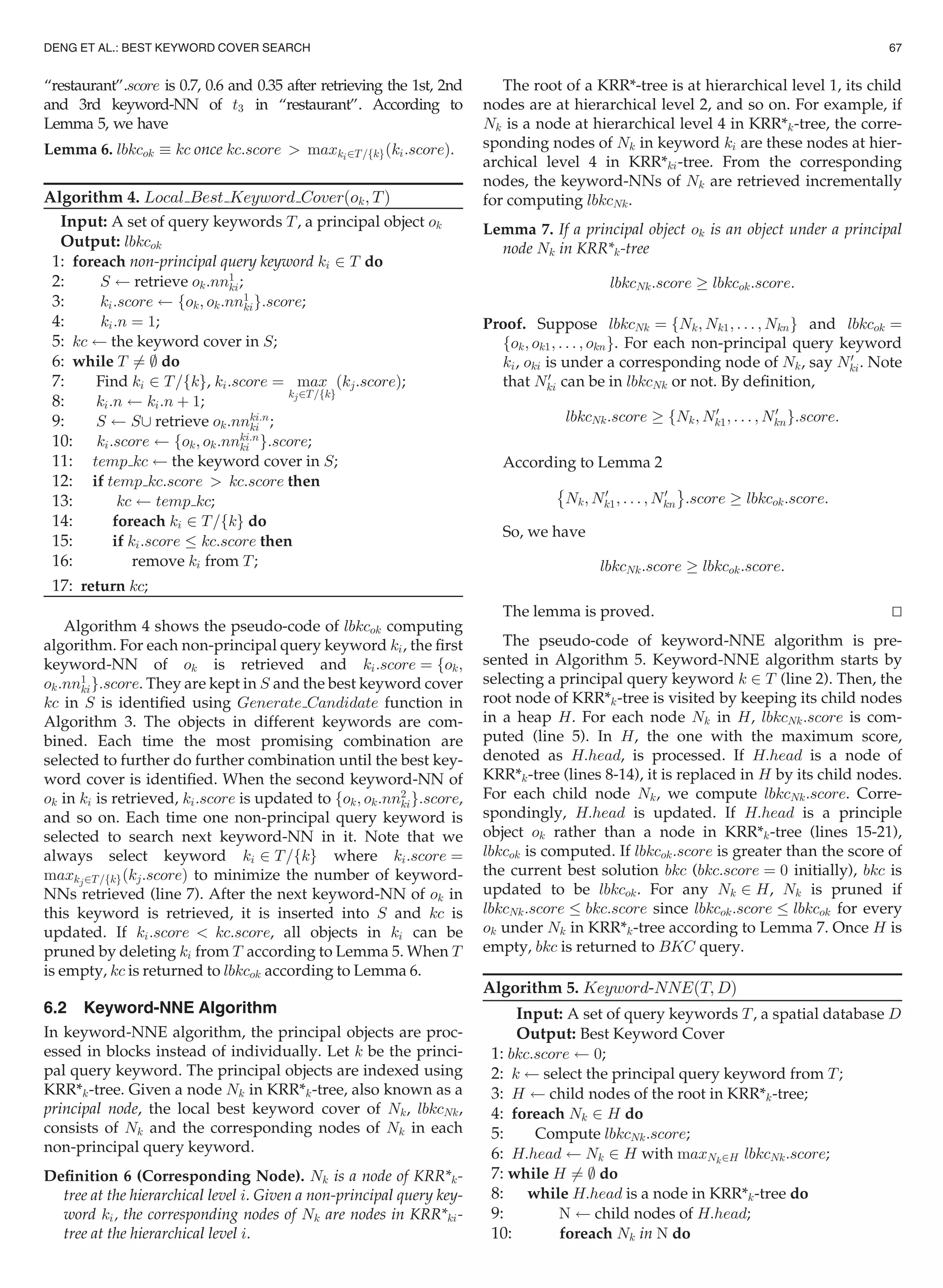
6.1.2 lbkc Computing Algorithm
Computing lbkcok is to incrementally retrieve keyword-
NNs of ok in each non-principal query keyword. An exam-
ple is shown in Fig. 4 where query keywords are “bar”,
“restaurant” and “hotel”. The principal query keyword is
“bar”. Suppose we are computing lbkct3. The first key-
word-NN of t3 in “restaurant” and “hotel” are c2 and s3
respectively. A set S is used to keep t3; s3; c2. Let kc be the
keyword cover in S which has the highest score (the idea
of Apriori algorithm can be used, see Section 5). After
step 1, kc:score ¼ 0:3. In step 2, “hotel” is selected and the
second keyword-NN of t3 in “hotel” is retrieved, i.e., s2.
Since ft3; s2g:score kc:score, s2 can be pruned and more
importantly all objects not accessed in “hotel” can be
pruned according to Lemma 5. In step 3, the second key-
word-NN of t3 in “restaurant” is retrieved, i.e., c3. Since
ft3; c3g:score kc:score, c3 is inserted into S. As a result,
kc is updated to 0:4. Then, the third keyword-NN of t3 in
“restaurant” is retrieved, i.e., c4. Since ft3; c4g:score
kc:score, c4 and all objects not accessed yet in “restaurant”
can be pruned according to Lemma 5. To this point, the
current kc is lbkct3.
Lemma 5. If kc:score fok; ok:nnt
kig, ok:nnt
ki and ok:nnt0
ki
(t0
t) must not be in lbkcok.
Proof. By definition, kc:score lbkcok:score. Since fok;
ok:nnt
kig:score kc:score, we have fok; ok:nnt
kig:score
lbkcok:score and in turn fok; ok:nnt0
kig:score lbkcok:
score. If ok:nnt
ki is in lbkcok, fok; ok:nnt
kig:score ! lbkcok:
score according to Lemma 1, so is ok:nnt0
ki. Thus, ok:nnt
ki
and ok:nnt0
ki must not be in lbkcok. tu
For each non-principal query keyword ki, after retrieving the
first t keyword-NNs of ok in keyword ki, we use ki:score
to denoted fok;ok:nnt
kig:score. For example in Fig. 4,
Fig. 3. Generating candidates.
Fig. 4. An example of lbkc computation.

“restaurant”.score is 0.7, 0.6 and 0.35 after retrieving the 1st, 2nd
and 3rd keyword-NN of t3 in “restaurant”. According to
Lemma 5, we have
Lemma 6. lbkcok kc once kc:score maxki2T=fkgðki:scoreÞ.
Algorithm 4. Local Best Keyword Coverðok; TÞ
Input: A set of query keywords T, a principal object ok
Output: lbkcok
1: foreach non-principal query keyword ki 2 T do
2: S retrieve ok:nn1
ki;
3: ki:score fok; ok:nn1
kig:score;
4: ki:n ¼ 1;
5: kc the keyword cover in S;
6: while T 6¼ ; do
7: Find ki 2 T=fkg, ki:score ¼ max
kj2T=fkg
ðkj:scoreÞ;
8: ki:n ki:n þ 1;
9: S S[ retrieve ok:nnki:n
ki ;
10: ki:score fok; ok:nnki:n
ki g:score;
11: temp kc the keyword cover in S;
12: if temp kc:score kc:score then
13: kc temp kc;
14: foreach ki 2 T=fkg do
15: if ki:score kc:score then
16: remove ki from T;
17: return kc;
Algorithm 4 shows the pseudo-code of lbkcok computing
algorithm. For each non-principal query keyword ki, the first
keyword-NN of ok is retrieved and ki:score ¼ fok;
ok:nn1
kig:score. They are kept in S and the best keyword cover
kc in S is identified using Generate Candidate function in
Algorithm 3. The objects in different keywords are com-
bined. Each time the most promising combination are
selected to further do further combination until the best key-
word cover is identified. When the second keyword-NN of
ok in ki is retrieved, ki:score is updated to fok; ok:nn2
kig:score,
and so on. Each time one non-principal query keyword is
selected to search next keyword-NN in it. Note that we
always select keyword ki 2 T=fkg where ki:score ¼
maxkj2T=fkgðkj:scoreÞ to minimize the number of keyword-
NNs retrieved (line 7). After the next keyword-NN of ok in
this keyword is retrieved, it is inserted into S and kc is
updated. If ki:score kc:score, all objects in ki can be
pruned by deleting ki from T according to Lemma 5. When T
is empty, kc is returned to lbkcok according to Lemma 6.
6.2 Keyword-NNE Algorithm
In keyword-NNE algorithm, the principal objects are proc-
essed in blocks instead of individually. Let k be the princi-
pal query keyword. The principal objects are indexed using
KRR*k-tree. Given a node Nk in KRR*k-tree, also known as a
principal node, the local best keyword cover of Nk, lbkcNk,
consists of Nk and the corresponding nodes of Nk in each
non-principal query keyword.
Definition 6 (Corresponding Node). Nk is a node of KRR*k-
tree at the hierarchical level i. Given a non-principal query key-
word ki, the corresponding nodes of Nk are nodes in KRR*ki-
tree at the hierarchical level i.
The root of a KRR*-tree is at hierarchical level 1, its child
nodes are at hierarchical level 2, and so on. For example, if
Nk is a node at hierarchical level 4 in KRR*k-tree, the corre-
sponding nodes of Nk in keyword ki are these nodes at hier-
archical level 4 in KRR*ki-tree. From the corresponding
nodes, the keyword-NNs of Nk are retrieved incrementally
for computing lbkcNk.
Lemma 7. If a principal object ok is an object under a principal
node Nk in KRR*k-tree
lbkcNk:score ! lbkcok:score:
Proof. Suppose lbkcNk ¼ fNk; Nk1; . . . ; Nkng and lbkcok ¼
fok; ok1; . . . ; okng. For each non-principal query keyword
ki, oki is under a corresponding node of Nk, say N0
ki. Note
that N0
ki can be in lbkcNk or not. By definition,
lbkcNk:score ! fNk; N0
k1; . . . ; N0
kng:score:
According to Lemma 2
È
Nk; N0
k1; . . . ; N0
kn
É
:score ! lbkcok:score:
So, we have
lbkcNk:score ! lbkcok:score:
The lemma is proved. tu
The pseudo-code of keyword-NNE algorithm is pre-
sented in Algorithm 5. Keyword-NNE algorithm starts by
selecting a principal query keyword k 2 T (line 2). Then, the
root node of KRR*k-tree is visited by keeping its child nodes
in a heap H. For each node Nk in H, lbkcNk:score is com-
puted (line 5). In H, the one with the maximum score,
denoted as H:head, is processed. If H:head is a node of
KRR*k-tree (lines 8-14), it is replaced in H by its child nodes.
For each child node Nk, we compute lbkcNk:score. Corre-
spondingly, H:head is updated. If H:head is a principle
object ok rather than a node in KRR*k-tree (lines 15-21),
lbkcok is computed. If lbkcok:score is greater than the score of
the current best solution bkc (bkc:score ¼ 0 initially), bkc is
updated to be lbkcok. For any Nk 2 H, Nk is pruned if
lbkcNk:score bkc:score since lbkcok:score lbkcok for every
ok under Nk in KRR*k-tree according to Lemma 7. Once H is
empty, bkc is returned to BKC query.
Algorithm 5. Keyword-NNEðT; DÞ
Input: A set of query keywords T, a spatial database D
Output: Best Keyword Cover
1: bkc:score 0;
2: k select the principal query keyword from T;
3: H child nodes of the root in KRR*k-tree;
4: foreach Nk 2 H do
5: Compute lbkcNk:score;
6: H:head Nk 2 H with maxNk2H lbkcNk:score;
7: while H 6¼ ; do
8: while H:head is a node in KRR*k-tree do
9: N child nodes of H:head;
10: foreach Nk in N do

11: Compute lbkcNk:score;
12: Insert Nk into H;
13: Remove H:head from H;
14: H:head Nk 2 H with maxNk2HlbkcNk:score;
= Ã H:head is a principal object (i.e., not a
node in KRR*k-tree)Ã=
15: ok H:head;
16: Compute lbkcok:score;
17: if bkc:score lbkcok:score then
18: bkc lbkcok;
19: foreach Nk in Hdo
20: if lbkcNk:score bkc:score then
21: Remove Nk from H;
22: return bkc;
7 WEIGHTED AVERAGE OF KEYWORD RATINGS
To this point, the minimum keyword rating of objects in O is
used in O:score. However, it is unsurprising that a user pre-
fers the weighted average of keyword ratings of objects in O
to measure O:score.
O:score ¼ a Â 1 À
diamðOÞ
max dist

þ ð1 À aÞ Â
W AverageðOÞ
max rating
;
(8)
where W AverageðOÞ is defined as
W AverageðOÞ ¼
P
oki2O wki Ã oki:rating
jOj
; (9)
where wki is the weight associated with the query keyword
ki and
P
ki2T wki ¼ 1. For example, a user may give higher
weight to “hotel” but lower weight to “restaurant” in a
BKC query. Given the score function in Equation (8), the
baseline algorithm and keyword-NNE algorithm can be
used to process BKC query with minor modification. The
core is to maintain the property in Lemmas 1 and in 2 which
are the foundation of the pruning techniques in the baseline
algorithm and the keyword-NNE algorithm.
However, the property in Lemma 1 is invalid given the
score function defined in Equation (9). To maintain this
property, if a combination does not cover a query keyword
ki, this combination is modified by inserting a virtual object
associated with ki. This virtual object does not change the
diameter of the combination, but it has the maximum rating
of ki (for the combination of nodes, a virtual node is inserted
in the similar way). The W AverageðOÞ is redefined to
W AverageÃ
ðOÞ.
W AverageÃ
ðOÞ ¼
E þ F
jTj
:
E ¼
X
oki2O
wki Ã oki:rating:
F ¼
X
kj2T=O:T
wkj Ã Okj:maxrating;
(10)
where T=O:T is the set of query keywords not covered by O,
Okj:maxrating is the maximum rating of objects in Okj. For
example in Fig. 1, suppose the query keywords are
“restaurant”, “hotel” and “bar”. For a combination
O ¼ ft1; c1g, W AverageðOÞ ¼ wt Ã t1:rating þ wc Ã c1:rating
while W AverageÃ
ðOÞ ¼ wt Ã t1:rating þ wc Ã c1:rating þ
ws Ã max ratings where wt; wc and ws are the weights
assigned to “bar”, “restaurant” and “hotel” respectively,
and max ratings is the highest keyword rating of objects in
“hotel”.
Given O:score with W AverageÃ
ðOÞ, it is easy to prove
that the property in Lemma 1 is valid. Note that the purpose
of W AverageÃ
ðOÞ is to apply the pruning techniques in the
baseline algorithm and keyword-NNE algorithm. It does
not affect the correctness of the algorithms. In addition, the
property in Lemma 2 is valid no matter which of
W AverageÃ
ðOÞ and W AverageðOÞ is used in O:score.
8 ANALYSIS
To help analysis, we assume a special baseline algorithm
BF-baseline which is similar to the baseline algorithm but the
best-first KRR*-tree browsing strategy is applied. For each
query keyword, the child nodes of the KRR*-tree root are
retrieved. The child nodes from different query keywords
are combined to generate candidate keyword covers (in the
same way as in the baseline algorithm, see Section 5) which
are stored in a heap H. The candidate kc 2 H with the maxi-
mum score is processed by retrieving the child nodes of kc.
Then, the child nodes of kc are combined to generate more
candidates which replace kc in H. This process continues
until a keyword cover consisting of objects only is obtained.
This keyword cover is the current best solution bkc. Any can-
didate kc 2 H is pruned if kc:score bkc:score. The remain-
ing candidates in H are processed in the same way. Once H
is empty, the current bkc is returned to BKC query. In
BF-baseline algorithm, only if a candidate keyword cover kc
has kc:score BKC:score, it is further processed by retriev-
ing the child nodes of kc and combining them to generate
more candidates.
8.1 Baseline
However, BF-baseline algorithm is not feasible in practice.
The main reason is that BF-baseline algorithm requires to
maintain H in memory. The peak size of H can be very large
because of the exhaustive combination until the first current
best solution bkc is obtained. To release the memory bottle-
neck, the depth-first browsing strategy is applied in the
baseline algorithm such that the current best solution is
obtained as soon as possible (see Section 5). Compared to
the best-first browsing strategy which is global optimal, the
depth-first browsing strategy is a kind of greedy algorithm
which is local optimal. As a consequence, if a candidate key-
word cover kc has kc:score bkc:score, kc is further proc-
essed by retrieving the child nodes of kc and combining
them to generate more candidates. Note that bkc:score
increases from 0 to BKC:score in the baseline algorithm.
Therefore, the candidate keyword covers which are further
processed in the baseline algorithm can be much more than
that in BF-baseline algorithm.
Given a candidate keyword cover kc, it is further proc-
essed in the same way in both the baseline algorithm and
BF-baseline algorithm, i.e., retrieving the child nodes of kc
and combine them to generate more candidates using

Generate Candidate function in Algorithm 3. Since the can-
didate keyword covers further processed in the baseline
algorithm can be much more than that in BF-baseline algo-
rithm, the total candidate keyword covers generated in
the baseline algorithm can be much more than that in
BF-baseline algorithm.
Note that the analysis captures the key characters of the
baseline algorithm in BKC query processing which are inher-
ited from the methods for mCK query processing [17], [18].
The analysis is still valid if directly extending the methods
[17], [18] to process BKC query as introduced in Section 4.
8.2 Keyword-NNE
In keyword-NNE algorithm, the best-first browsing strategy
is applied like BF-baseline but large memory requirement
is avoided. For the better explanation, we can imagine all
candidate keyword covers generated in BF-baseline algo-
rithm are grouped into independent groups. Each group is
associated with one principal node (or object). That is, the
candidate keyword covers fall in the same group if they
have the same principal node (or object). Given a principal
node Nk, let GNk be the associated group. The example in
Fig. 5 shows GNk where some keyword covers such as
kc1; kc2 have score greater than BKC:score, denoted as G1
Nk,
and some keyword covers such as kc3; kc4 have score not
greater than BKC:score, denoted as G2
Nk. In BF-baseline
algorithm, GNk is maintained in H before the first current
best solution is obtained, and every keyword cover in G1
Nk
needs to be further processed.
In keyword-NNE algorithm, the keyword cover in GNk
with the highest score, i.e., lbkcNk, is identified and main-
tained in memory. That is, each principal node (or object)
keeps its lbkc only. The total number of principal nodes (or
objects) is Oðn log nÞ where n is the number of principal
objects. So, the memory requirement for maintaining H is
Oðn log nÞ. The (almost) linear memory requirement makes
the best-first browsing strategy practical in keyword-NNE
algorithm. Due to the best-first browsing strategy, lbkcNk is
further processed in keyword-NNE algorithm only if
lbkcNk:score BKC:score.
8.2.1 Instance Optimality
The instance optimality [6] corresponds to the optimality in
every instance, as opposed to just the worst case or the aver-
age case. There are many algorithms that are optimal in a
worst-case sense, but are not instance optimal. An example
is binary search. In the worst case, binary search is guaran-
teed to require no more than log N probes for N data items.
By linear search which scans through the sequence of data
items, N probes are required in the worst case. However,
binary search is not better than linear search in all instances.
When the search item is in the very first position of the
sequence, a positive answer can be obtained in one probe
and a negative answer in two probes using linear search.
The binary search may still require log N probes.
Instance optimality can be formally defined as follows: for
a class of correct algorithms A and a class of valid input D to
the algorithms, costðA; DÞ represents the amount of a
resource consumed by running algorithm A 2 A on input
D 2 D. An algorithm B 2 A is instance optimal over A and
D if costðB; DÞ ¼ OðcostðA; DÞÞ for 8A 2 A and 8D 2 D.
This cost could be running time of algorithm A over input D.
Theorem 1. Let D be the class of all possible spatial databases
where each tuple is a spatial object and is associated with a key-
word. Let A be the class of any correct BKC processing algo-
rithm over D 2 D. For all algorithms in A, multiple KRR*-
trees, each for one keyword, are explored by combining nodes
at the same hierarchical level until leaf node, and no combina-
tion of objects (or nodes of KRR*-trees) has been pre-processed,
keyword-NNE algorithm is optimal in terms of the number of
candidate keyword covers which are further processed.
Proof. Due to the best-first browsing strategy, lbkcNk is
further processed in keyword-NNE algorithm only if
lbkcNk:score BKC:score. In any algorithm A 2 A, a
number of candidate keyword covers need to be gen-
erated and assessed since no combination of objects
(or nodes of KRR*-trees) has been pre-processed.
Given a node (or object) N, the candidate keyword
covers generated can be organized in a group if they
contain N. In this group, if one keyword cover has
score greater than BKC:score, the possibility exists
that the solution of BKC query is related to this
group. In this case, A needs to process at least one
keyword cover in this group. If A fails to do this, it
may lead to an incorrect solution. That is, no algo-
rithm in A can process less candidate keyword covers
than keyword-NNE algorithm. tu
8.2.2 Candidate Keyword Covers Processing
Every candidate keyword cover in G1
Nk is further processed
in BF-baseline algorithm. In the example in Fig. 5, kc1 is fur-
ther processed, so does every kc 2 G1
Nk. Let us look closer at
kc1 ¼ fNk; Nk1; Nk2g processing. As introduced in Section 4,
each node N in KRR*-tree is defined as Nðx; y; r; lx; ly; lrÞ
which can be represented with 48 bytes. If the disk pagesize
is 4,096 bytes, the reasonable fan-out of KRR*-tree is 40-50.
That is, each node in kc1 (i.e., Nk, Nk1 and Nk2) has 40-50
Fig. 5. BF-baseline versus keyword-NNE.

child nodes. In kc1 processing in BF-baseline algorithm,
these child nodes are combined to generate candidate key-
word covers using Algorithm 3.
In keyword-NNE algorithm, one and only one key-
word cover in G1
Nk, i.e., lbkcNk, is further processed. For
each child node cNk of Nk, lbkccNk is computed. For com-
puting lbkccNk, a number of keyword-NNs of cNk are
retrieved and combined to generate more candidate key-
word covers using Algorithm 3. The experiments on real
data sets illustrate that only 2-4 keyword-NNs in average
in each non-principal query keyword are retrieved in
lbkccNk computation.
When further processing a candidate keyword cover,
keyword-NNE algorithm typically generates much less new
candidate keyword covers compared to BF-baseline algo-
rithm. Since the number of candidate keyword covers
further processed in keyword-NNE algorithm is optimal
(Theorem 1), the number of keyword covers generated in
BF-baseline algorithm is much more than that in keyword-
NNE algorithm. In turn, we conclude that the number of
keyword covers generated in baseline algorithm is much
more than that in keyword-NNE algorithm. This conclusion
is independent of the principal query keyword since the
analysis does not apply any constraint on the selection strat-
egy of principal query keyword.
9 EXPERIMENT
In this section we experimentally evaluate keyword-NNE
algorithm and the baseline algorithm. We use four real data
sets, namely Yelp, Yellow Page, AU, and DE. Specifically,
Yelp is a data set extracted from Yelp Academic Data Set
(www.yelp.com) which contains 7,707 POIs (i.e., points of
interest, which are equivalent to the objects in this work)
with 27 keywords where the average, maximum and mini-
mum number of POIs in each keyword are 285, 1,353 and
120 respectively. Yellow Page is a data set obtained from
yellowpage.com.au in Sydney which contains 30,444 POIs
with 26 keywords where the average, maximum and mini-
mum number of POIs in each keyword are 1,170, 10,284 and
154 respectively. All POIS in Yelp has been rated by custom-
ers from 1 to 10. About half of the POIs in Yellow Page have
been rated by Yelp, the unrated POIs are assigned average
rating 5. AU and US are extracted from a public source.2
AU contains 678,581 POIs in Australia with 187 keywords
where the average, maximum and minimum number of
POIs in each keyword are 3,728, 53,956 and 403 respectively.
US contains 1,541,124 POIs with 237 keywords where the
average, maximum and minimum number of POIs in each
keyword are 6,502, 122,669 and 400. In AU and US, the key-
word ratings from 1 to 10 are randomly assigned to POIs.
The ratings are in normal distribution where the mean
m ¼ 5 and the standard deviation s ¼ 1. The distribution of
POIs in keywords are illustrated in Fig. 6. For each data set,
the POIs of each keyword are indexed using a KRR*-tree.
We are interested in 1) the number of candidate keyword
covers generated, 2) BKC query response time, 3) the maxi-
mum memory consumed, and 4) the average number of
keyword-NNs of each principal node (or object) retrieved
for computing lbkc and the number of lbkcs computed for
answering BKC query. In addition, we test the performance
in the situation that the weighted average of keyword rat-
ings is applied as discussed in Section 7. All algorithms are
implemented in Java 1.7.0. and all experiments have been
performed on a Windows XP PC with 3.0 Ghz CPU and
3 GB main memory.
In Fig. 7, the number of keyword covers generated in
baseline algorithm is compared to that in the algorithms
directly extended from [17], [18] when the number of query
keywords m changes from 2 to 9. It shows that the baseline
algorithm has better performance in all settings. This is con-
sistent with the analysis in Section 5. The test results on Yel-
low Page and Yelp data sets are shown in Fig. 7a which
represents data sets with small number of keywords. The
test results on AU and US data sets are shown in Fig. 7b
which represents data set with large number of keywords.
As observed, when the number of keywords in a data set is
small, the difference between baseline algorithm and the
directly extended algorithms is reduced. The reason is that
the single tree index in the directly extended algorithms has
more pruning power in this case (as discussed in Section 4).
9.1 Effect of mmm
The number of query keywords m has significant impact to
query processing efficiency. In this test, m is changed from
2 to 9 when a ¼ 0:4. Each BKC query is generated by ran-
domly selecting m keyword from all keywords as the query
Fig. 6. The distribution of keyword size in test data sets.
Fig. 7. Baseline, Virtual bR*-tree and bR*-tree.
2. http://s3.amazonaws.com/simplegeo-public/places_dump_20110628.
zip.

keywords. For each setting, we generate and perform 100
BKC queries, and the averaged results are reported.3
Fig. 8
shows the number of candidate keyword covers generated
for BKC query processing. When m increases, the number
of candidate keyword covers generated increases dramati-
cally in the baseline algorithm. In contrast, keyword-NNE
algorithm shows much better scalability. The reason has
been explained in Section 8.
Fig. 9 reports the average response time of BKC query
when m changes. The response time is closely related to the
candidate keyword covers generated during the query proc-
essing. In the baseline algorithm, the response time
increases very fast when m increases. This is consistent with
the fast increase of the candidate keyword covers generated
when m increases. Compared to the baseline algorithm, the
keyword-NNE algorithm shows much slower increase
when m increases.
For processing the BKC queries at the same settings of m
and a, the performances are different on data sets US, AU,
YELP and Yellow Page as shown in Figs. 8 and 9. The reason
is that the average number of objects in one keyword in data
sets US, AU, YELP and Yellow Page are 6,502, 3,728, 1,170
and 285 respectively as shown in Fig. 6; in turn, the average
numbers of objects in one query keyword in the BKC queries
on data set US, AU, YELP and Yellow Page are expected to be
the same. The experimental results show the higher average
number such as on data set US leads to the more candidate
keyword covers and the more processing time.
9.2 Effect of a
This test shows the impact of a to the performance. As
shown in Equation (2), a is an application speciﬁc parameter
to balance the weight of keyword rating and the diameter in
the score function. Compared to m, the impact of a to the
performance is limited. When a ¼ 1, BKC query is
degraded to mKC query where the distance between objects
is the sole factor and keyword rating is ignored. When a
changes from 1 to 0, more weight is assigned to keyword
rating. In Fig. 10, an interesting observation is that with the
decrease of a the number of keyword covers generated in
both the baseline algorithm and keyword-NNE algorithm
shows a constant trend of slight decrease. The reason
behind is that KRR*-tree has a keyword rating dimension.
Objects close to each other geographically may have very
different ratings and thus they are in different nodes of
KRR*-tree. If more weight is assigned to keyword ratings,
KRR*-tree tends to have more pruning power by distin-
guishing the objects close to each other but with different
keyword ratings. As a result, less candidate keyword covers
are generated. Fig. 11 presents the average response time of
queries which are consistent with the number of candidate
keyword covers generated.
BKC query provides robust solutions to meet various
practical requirements while mCK query cannot. Suppose
we have three query keywords in Yelp data set, namely,
“bars”, “hotels and travel”, and “fast food”. When a ¼ 1,
the BKC query (equivalent to mCK query) returns Pita
House, Scottsdale Neighborhood Trolley, and Schlotzskys (the
names of the selected objects in keyword “bars”, “hotels
and travel”, and “fast food” respectively) where the lowest
keyword rating is 2.5 and the maximum distance is 0.045
km. When a ¼ 0:4, the BKC query returns The Attic, Enter-
prise Rent-A-Car and Chick-Fil-A where the lowest keyword
rating is 4.5 and the maximum distance is 0.662 km.
9.3 Maximum Memory Consumption
The maximum memory consumed by the baseline algo-
rithm and keyword-NNE algorithm are reported in Fig. 12
(the average results of 100 BKC queries on each of four
data sets). It shows that the maximum memory consumed
in keyword-NNE algorithm is up to 0.5 MB in all settings of
m while it increases very fast when m increases in the base-
line algorithm. As discussed in Section 8, keyword-NNE
algorithm only maintains the principal nodes (or objects) in
Fig. 9. Response time versus m (a ¼ 0.4).
Fig. 8. Number of candidate keyword covers generated versus m (a ¼ 0.4).
3. In this work, all experimental results are obtained in the same
way.

memory while the baseline algorithm maintains candidate
keyword covers in memory.
9.4 Keyword-NNE
The high performance of keyword-NNE algorithm is due to
that each principal node (or object) only retrieves a few key-
word-NNs in each non-principal query keyword. Suppose
all retrieved keyword-NNs in keyword-NNE algorithm are
kept in a set S. In Fig. 13a, the average size of S is shown.
The data sets are randomly sampled so that the number of
objects in each query keyword in a BKC query is from 100
to 3,000. It illustrates that the impact of the number of
objects in query keywords to the size of S is limited. On the
contrary, it shows that the size of S is clearly inﬂuenced by
m. When m increases from 2 to 9, S increases linearly. In
average, a principal node (or object) only retrieves 2-4 key-
word-NNs in each non-principal query keyword. Fig. 13b
shows the number of lbkcs computed in query processing.
We can see less than 10 percent of principal nodes (or
objects) need to compute their lbkcs in different sizes of data
sets. In other words, 90 percent of the overall principal
nodes (or objects) are pruned during the query processing.
9.5 Weighted Average of Keyword Ratings
The tests compare the weighted average of keyword rating
and the minimum keyword rating to performance. The
average experimental results of 100 BKC queries on each of
four data sets are reported in Fig. 14. We can see the differ-
ence between these two situations is trivial. This is because
the score computation in the situation of the minimum key-
word rating is fundamentally equivalent to that in the situa-
tion of weight average. In the former situation, if a
combination O of objects (or their MBRs) does not cover a
keyword, the rating of this keyword used for computing
O:score is 0 while it is the maximum rating of this keyword
in the latter situation.
10 CONCLUSION
Compared to the most relevant mCK query, BKC query
provides an additional dimension to support more sensible
decision making. The introduced baseline algorithm is
inspired by the methods for processing mCK query. The
baseline algorithm generates a large number of candidate
keyword covers which leads to dramatic performance drop
when more query keywords are given. The proposed key-
word-NNE algorithm applies a different processing strat-
egy, i.e., searching local best solution for each object in a
certain query keyword. As a consequence, the number of
candidate keyword covers generated is signiﬁcantly
reduced. The analysis reveals that the number of candidate
keyword covers which need to be further processed in
Fig. 10. Number of candidate keyword covers generated versus aðm ¼ 4Þ.
Fig. 11. Response time versus aðm ¼ 4Þ.
Fig. 12. Maximum memory consumed versus m (a ¼ 0.4). Fig. 13. Features of keyword-NNE (a ¼ 0.4).

keyword-NNE algorithm is optimal and processing each
keyword candidate cover typically generates much less
new candidate keyword covers in keyword-NNE algorithm
than in the baseline algorithm.
ACKNOWLEDGMENTS
This research was partially supported by Natural Science
Foundation of China (Grant No. 61232006), the Australian
Research Council (Grants No. DP110103423 and No.
DP120102829), and 863 National High-Tech Research Plan
of China (No. 2012AA011001).
REFERENCES
[1] R. Agrawal and R. Srikant, “Fast algorithms for mining associa-
tion rules in large databases,” in Proc. 20th Int. Conf. Very Large
Data Bases, 1994, pp. 487–499.
[2] T. Brinkhoff, H. Kriegel, and B. Seeger, “Efficient processing of
spatial joins using r-trees,” in Proc. ACM SIGMOD Int. Conf. Man-
age. Data, 1993, pp. 237–246.
[3] X. Cao, G. Cong, and C. Jensen, “Retrieving top-k prestige-based
relevant spatial web objects,” Proc. VLDB Endowment, vol. 3, nos.
1/2, pp. 373–384, Sep. 2010.
[4] X. Cao, G. Cong, C. Jensen, and B. Ooi, “Collective spatial key-
word querying,” in Proc. ACM SIGMOD Int. Conf. Manage. Data,
2011, pp. 373–384.
[5] G. Cong, C. Jensen, and D. Wu, “Efficient retrieval of the top-k
most relevant spatial web objects,” Proc. VLDB Endowment, vol. 2,
no. 1, pp. 337–348, Aug. 2009.
[6] R. Fagin, A. Lotem, and M. Naor, “Optimal aggregation algo-
rithms for middleware,” J. Comput. Syst. Sci., vol. 66, pp. 614–656,
2003.
[7] I. D. Felipe, V. Hristidis, and N. Rishe, “Keyword search on
spatial databases,” in Proc. IEEE 24th Int. Conf. Data Eng.,
2008, pp. 656–665.
[8] R. Hariharan, B. Hore, C. Li, and S. Mehrotra, “Processing spatial-
keyword (SK) queries in geographic information retrieval (GIR)
systems,” in Proc. 19th Int. Conf. Sci. Statist. Database Manage.,
2007, pp. 16–23.
[9] G. R. Hjaltason and H. Samet, “Distance browsing in spatial data-
bases,” ACM Trans. Database Syst., vol. 24, no. 2, pp. 256–318, 1999.
[10] Z. Li, K. C. Lee, B. Zheng, W.-C. Lee, D. Lee, and X. Wang, “IR-
Tree: An efficient index for geographic document search,” IEEE
Trans. Knowl. Data Eng., vol. 99, no. 4, pp. 585–599, Apr. 2010.
[11] N. Mamoulis and D. Papadias, “Multiway spatial joins,” ACM
Trans. Database Syst., vol. 26, no. 4, pp. 424–475, 2001.
[12] D. Papadias, N. Mamoulis, and B. Delis, “Algorithms for querying
by spatial structure,” in Proc. Int. Conf. Very Large Data Bases, 1998,
pp. 546–557.
[13] D. Papadias, N. Mamoulis, and Y. Theodoridis, “Processing and
optimization of multiway spatial joins using r-trees,” in Proc. 18th
ACM SIGMOD-SIGACT-SIGART Symp. Principles Database Syst.,
1999, pp. 44–55.
[14] J. M. Ponte and W. B. Croft, “A language modeling approach to
information retrieval,” in Proc. 21st Annu. Int. ACM SIGIR Conf.
Res. Develop. Inf. Retrieval, 1998, pp. 275–281.
[15] J. Rocha-Junior, O. Gkorgkas, S. Jonassen, and K. Nørva

g,
“Efficient processing of top-k spatial keyword queries,” in Proc.
12th Int. Conf. Adv. Spatial Temporal Databases, 2011, pp. 205–222.
[16] S. B. Roy and K. Chakrabarti, “Location-aware type ahead
search on spatial databases: Semantics and efficiency,” in Proc.
ACM SIGMOD Int. Conf. Manage. Data, 2011, pp. 361–372.
[17] D. Zhang, B. Ooi, and A. Tung, “Locating mapped resources in
web 2.0,” in Proc. IEEE 26th Int. Conf. Data Eng., 2010, pp. 521–532.
[18] D. Zhang, Y. Chee, A. Mondal, A. Tung, and M. Kitsuregawa,
“Keyword search in spatial databases: Towards searching by doc-
ument,” in Proc. IEEE Int. Conf. Data Eng., 2009, pp. 688–699.
Ke Deng received the master’s degree in informa-
tion and communication technology from Griffith
University, Australia, in 2001, and the PhD degree
in computer science from the University of
Queensland, Australia, in 2007. His research
background include high-performance database
system, spatio-temporal data management, data
quality control, and business information system.
His current research interest include big spatio-
temporal data management and mining.
Xin Li received the bachelor’s degree from the
School of Information at the Renmin University
of China in 2007, and is currently working tow-
rard the master’s degree in computer science at
the Renmin University of China. His current
research interests include spatial database and
geo-positioning.
Jiaheng Lu received the MS degree from
Shanghai Jiaotong University in 2001 and the
PhD degree from the National University of
Singapore in 2007. He is a professor of com-
puter science at the Renmin University of
China. His research interests include many
aspects of data management. His current
research focuses on developing an academic
search engine, XML data management, and big
data management. He was in the organization
and program committees for various conferen-
ces, including SIGMOD, VLDB, ICDE, and CIKM.
Xiaofang Zhou received the BS and MS degrees
in computer science from Nanjing University,
China, in 1984 and 1987, respectively, and the
PhD degree in computer science from the Univer-
sity of Queensland, Australia, in 1994. He is a pro-
fessor of computer science with the University of
Queensland. He is the head of the Data and
Knowledge Engineering Research Division,
School of Information Technology and Electrical
Engineering. He is also an specially appointed
adjunct professor at Soochow University, China.
From 1994 to 1999, he was a senior research scientist and project
leader in CSIRO. His research is focused on finding effective and effi-
cient solutions to managing integrating, and analyzing very large
amounts of complex data for business and scientific applications. His
research interests include spatial and multimedia databases, high-
performance query processing, web information systems, data mining,
and data quality management. He is a senior member of the IEEE.
For more information on this or any other computing topic,
please visit our Digital Library at www.computer.org/publications/dlib.
Fig. 14. Weighted average versus minimum (a ¼ 0:4Þ.

Best Keyword Cover Search

More Related Content

What's hot

Similar to Best Keyword Cover Search

Recently uploaded

Best Keyword Cover Search