Download as PDF, PPTX

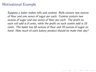
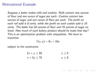
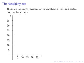
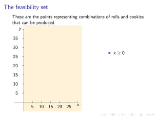
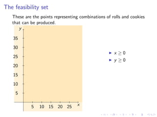
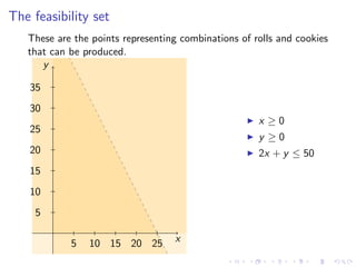
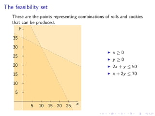
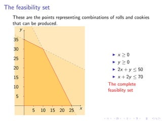

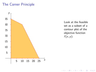
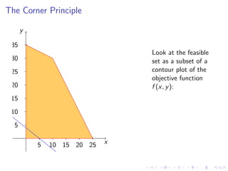

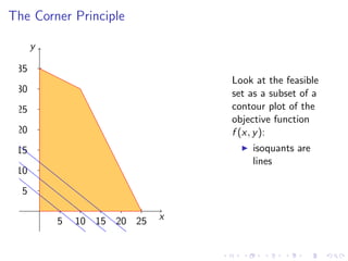
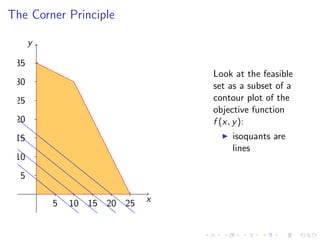


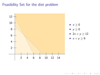
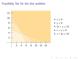
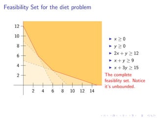

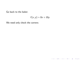
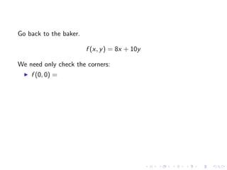
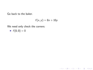
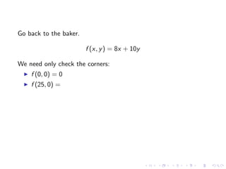

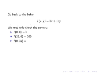
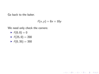
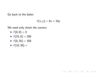
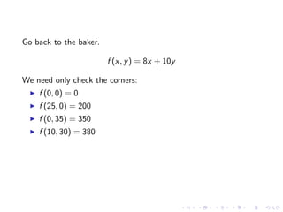
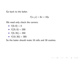
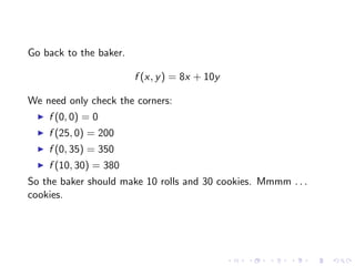
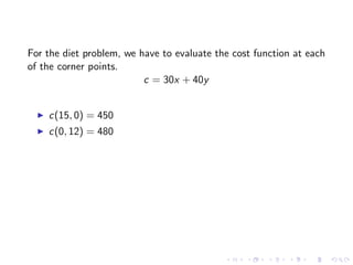
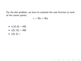
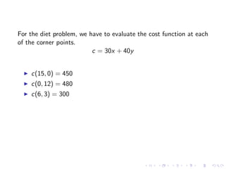
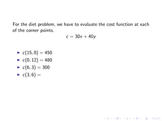


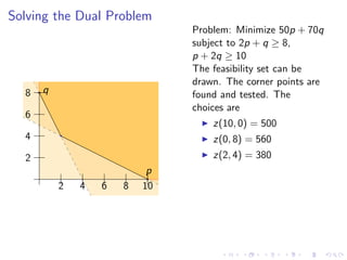
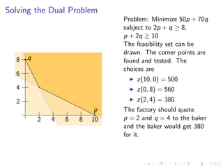
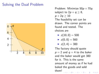

Lesson 29 covers linear programming and the corner principle, emphasizing its application in optimization problems such as those faced by a baker and a nutritionist. The document discusses maximizing profits by determining the best combinations of products under given constraints, as well as evaluating different cost scenarios for meal planning. Key concepts include the feasibility set, evaluation of corner points, and the relationship between linear programming and optimization.