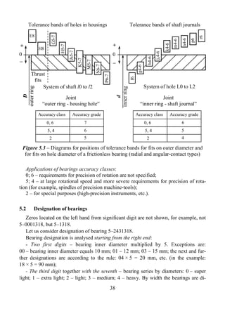
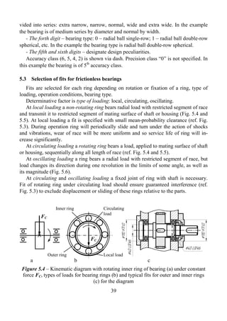
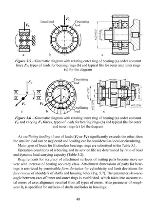
The document outlines the basics of interchangeability and the unified system of tolerances and fits, essential for mechanical engineering students. It covers norms for various connections, measurements, quality control methods, and the significance of standardization in ensuring reliable part production. The content serves as a foundation for further specialized studies in machine design and manufacturing processes.


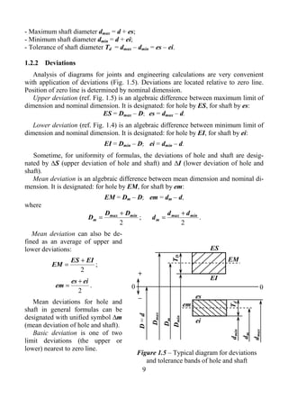


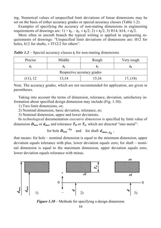


![Table 4.1 – Statistical characteristics of random errors for batch of parts
Statistical
Definition, formula
characteristic
Empirical centre of grouping or arithmetic mean of considered pa-
1 n
xm rameter values, x m = ∑ x i , assumed as a true value of measured
n 1
parameter
Statistical expectation – theoretically constant parameter, character-
M(x)
ises centre of scatter of random errors, M(x) ≈ xm
∆xi Absolute error, ∆xi = xi – xm
Scatter band, v = xmax – xmin, where xmax and xmin – maximum and
v
minimum actual (measured) dimensions, respectively
Standard deviation of random values of parameter from grouping cen-
σ tre, dimension parameter. It is a convenient characteristic for estima-
tion of random errors values
Mean-square error for n measurements, S n =
1 n
∑
n −1 1
( )2
x i − x m . If
number of observations (measurements) is very large, then
Sn
Sn → σ, that is, σ = lim S n (statistical limit). In reality one always
n →∞
calculates not σ, but its approximate value Sn , which is nearer to σ
with n increase
Dispersion, D = σ 2. It characterises degree of scatter of random errors
around scatter centre.
1 n
D Sample variance S n =2
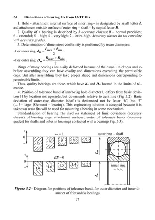
∑ ( xi − x m )2 .
n −1 1
General dispersion σ 2 = lim S n .
2
n →∞
−
(∆x ) 2
1 2 t
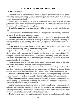
y Probability density, y = e 2σ or у = ,
σ 2π σ
dimension function ([1/mm], [1/µm], etc.)
Probability, integral of the y function, Pα = P(–∆x ≤ ∆x ≤ +∆x) for
confidence interval from (–∆x) to (+∆x). It characterises level of reli-
Pα
ability of obtained result. It is an area under the distribution curve
bounded by abscissa axis and limits of interval
Risk, sum of two quantiles, Pβ = (1 – Pα)·100%,
Pβ
Pβ = 0.27 % at Pα = 0.9973
32](https://image.slidesharecdn.com/basicsofinterchangeability-120508070541-phpapp02/85/Basics-of-interchangeability-32-320.jpg)


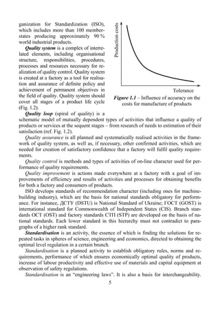
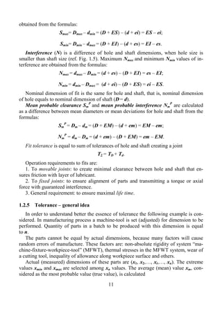
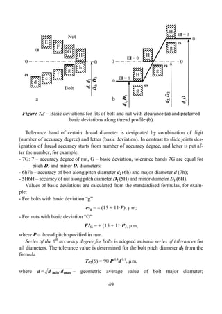
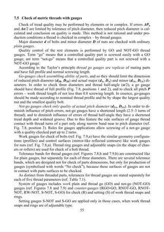
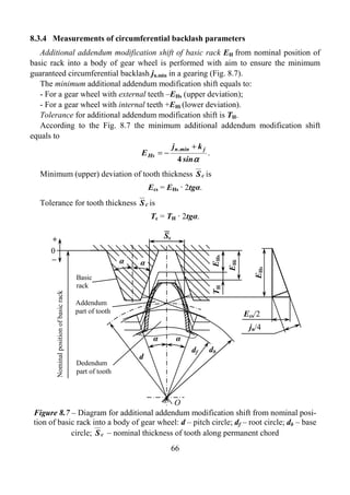
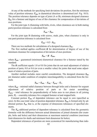
![6 DIMENSION CHAINS
For proper operation of machines or mechanisms it is necessary that their constituent
parts and surfaces of these parts occupy definite positions relative each other that corre-
spond to design purpose.
6.1 Fundamentals of theory of dimension chains
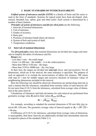
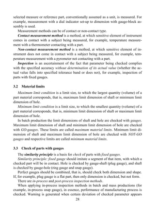
Dimension chain is a system of interconnected dimensions, which determine relative
positions of surfaces of one or several parts and create close contour.
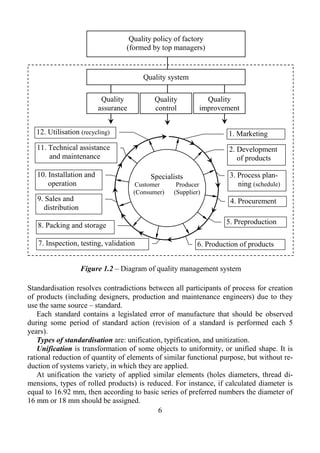
Dimensions included into dimension chain are called links, which are designated in
diagrams with capital letters with indexes, for example, A1, A2, A3, AΣ (Fig. 6.1).
Dimension chains are divided to:
- Related to a part;
- Related to an assembly (ref. Fig. 6.1);
- Linear;
- Angular;
- Design;
- Manufacturing;
- Measuring (metrological).
Linear dimension chains are divided to:
AΣ A3
- Spatial;
- Flat: with parallel links (collinear) (ref. Fig. 6.1)
A1 and with non-parallel links.
a A2 Links of dimension chain are divided to:
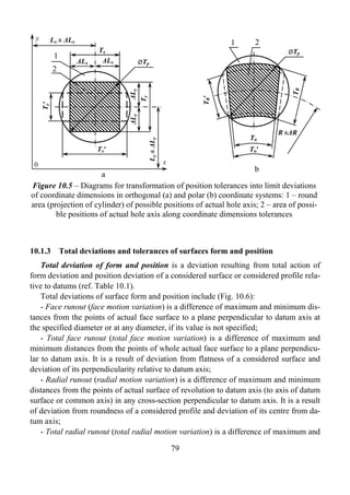
← ← - Initial, [AΣ];
A1 [А∑] A3 - Closing, AΣ;
→
→
A2 - Constituent links: increasing, A2 ; decreasing,
← ←
b A1 , A3 (ref. Fig. 6.1).
Figure 6.1 – Fragment of Constituent (increasing and decreasing) are called
drawing (a) and diagram of those links of dimension chain, change of which re-
dimension chain (b) sults in change of closing link AΣ, but can not and
should not change initial link [AΣ]. Enlargement of
increasing link enlarges value of closing link, and
enlargement of decreasing link reduces value of closing link.
Initial [AΣ] is called that link, to which basic requirement for accuracy is submitted
and which determines quality of an item. It is specified by designer nominal dimension
with tolerance, limit deviations, which should be ensured as a result of solution of di-
mension chain. This term (initial link) is used in design calculations.
42](https://image.slidesharecdn.com/basicsofinterchangeability-120508070541-phpapp02/85/Basics-of-interchangeability-42-320.jpg)
![In manufacturing process of machining or assembling of an item the initial link is
obtained last and thus it closes the dimension chain. Therefore in technological calcula-
tions it is called closing link AΣ. This term (closing link) is used in check calculations.
Calculations and analysis of dimension chains is an obligatory stage of designing
and manufacture of machines, which enhances providing of interchangeability, reduc-
tion of labour expenditures, quality improvements.
Essence of dimension chains calculations is in determination of nominal dimensions,
tolerances and limit deviations for all links under the requirements of design or tech-
nology.
Completeness (closure) of dimension chain is a necessary condition for starting the
calculations
m → n ←
AΣ = ∑ A j − ∑ Aq ,
1 1
→ ←
where A j – increasing links; Aq – decreasing links; m – number of increasing links; n
– number of decreasing links.
For example, for the diagram depicted in Fig. 6.1 the equation of dimension chain is
→ ← ←
AΣ = A2 − A1 + A3 .
When calculating dimension chains 2 types of tasks are solved:
1) Determination of nominal dimension, tolerance and limit deviations for closing
link AΣ from the given nominal dimensions and limit deviations of constituent links –
check calculations;
2) Determination of nominal dimension, tolerance and limit deviations for desired
constituent link from other known dimensions of chain and given initial dimension [AΣ]
– design calculations.
6.2 Procedure for design calculations of dimension chains
1. Plot the diagram of dimension chain from the drawing.
2. Find the initial link [AΣ]. Determine its nominal dimension, limit deviations, tol-
erance [TΣ], middle coordinate of tolerance band (mean deviation).
3. Find constituent links (increasing and decreasing).
4. Compile main equation of dimension chain (closeness equation), calculate nomi-
nal dimensions of all links Ai including the dependent link AX. When selecting a de-
pendent link the condition of minimal production costs is taken into account.
5. Select method and technique to ensure the given accuracy of closing link AΣ.
Methods for ensuring a specified accuracy of closing link:
1) Maximum-minimum method – for complete interchangeability;
43](https://image.slidesharecdn.com/basicsofinterchangeability-120508070541-phpapp02/85/Basics-of-interchangeability-43-320.jpg)
![2) Probabilistic method – for incomplete interchangeability (for example, risk
Pβ = 0.27 % provides low production costs);
3) Other methods: fitting, adjustment, etc.
Techniques for ensuring a specified accuracy of closing link: a) of equal tolerances;
b) of equal accuracy grades.
6. Calculate tolerance for each constituent link Ai:
a) Technique of equal tolerances: Calculate the mean value of tolerance Tmi for each
constituent link:
1) Maximum-minimum method: Tmi = Σ ;
[T ]
m+n
2) Probabilistic method: Tmi =
[TΣ ] ,
m+n
where [TΣ] – tolerance of initial link (specified in a drawing), m – number of increasing
links; n – number of decreasing links.
Taking into account the calculated Tmi values assign the nearest standard tolerance
values Ti for each constituent link Ai (except AX) with determination of accuracy
grades;
b) Technique of equal accuracy grades: Select values of tolerance units ii for each con-
stituent link Ai from the standard by their nominal dimensions. Determine mean level
of accuracy for all constituent links with mean number am calc of tolerance units:
1) Maximum-minimum method: a m calc =
[TΣ ] ;
∑ ii
2) Probabilistic method: a m calc =
[TΣ ] .
∑ i i2
According to the calculations result the nearest standardised value аm and respective
accuracy grade are accepted (ref. Table 2.2). Tolerance Ti for each link Ai (including
AX) is selected from the standard by their nominal dimensions and accuracy grade.
7. Check validity of determined tolerances and perform corrections, if necessary.
Tolerance of closing link TΣ should be less or equal to the tolerance of initial link
TΣ ≤ [TΣ].
Tolerance of closing link is determined from the formulas:
m+n
- TΣ = ∑ Ti , when calculating with maximum-minimum method;
1
m +n
- TΣ = ∑ Ti2 , when calculating with probabilistic method.
1
44](https://image.slidesharecdn.com/basicsofinterchangeability-120508070541-phpapp02/85/Basics-of-interchangeability-44-320.jpg)
![Corrections are made by assigning higher accuracy (smaller number of accuracy
grade) and, hence, smaller tolerance value to one or more constituent links.
8. Assign tolerance bands for each constituent link Ai (except AX) according to the
accuracy grade and type of dimension (for holes – Н basic deviation, for shafts – h, for
others – js).
9. From the standard for each constituent link Ai (except AX) determine limit devia-
tions and calculate mean deviations
∆mi = (∆Si + ∆Ii)/2,
where ∆Si – upper deviation of Ai nominal dimension; ∆Ii – lower deviation.
10. Determine middle coordinate of tolerance band ∆mX of dependent link AX from
the formula
m → n ←
[∆m Σ ] = ∑ ∆m j − ∑ ∆m q ,
1 1
where [∆mΣ] – mean deviation of [AΣ] initial link.
Mean deviation ∆mX can be in the group of increasing links or in the group of de-
ceasing links.
11. According to the nominal dimension AX, accepted accuracy grade and tolerance
TX select in the standard the tolerance band with mean deviation
∆mST = (∆SST + ∆IST)/2 nearest to the calculated deviation ∆mX.
12. In order to check correctness of the selection calculate mean deviation ∆mΣ of
closing link with the ∆mST selected value. Mean deviation ∆mΣ should be as near to the
mean deviation [∆mΣ] of initial link as possible
m → n ←
∆m Σ = ∑ ∆m j − ∑ ∆m q → [∆mΣ].
1 1
13. In order to check correctness of constituent links parameters calculate the upper
∆SΣ and lower ∆IΣ deviations of closing link and limit dimensions AΣmax and AΣmin of
closing link:
∆SΣ = ∆mΣ + 0.5TΣ; ∆IΣ = ∆mΣ – 0.5TΣ;
AΣmax = AΣ + ∆SΣ; AΣmin = AΣ + ∆IΣ,
where AΣ – nominal dimension of closing link equals nominal dimension of initial link
[AΣ].
If the calculated values satisfy conditions AΣmax ≤ [AΣmax] and AΣmin ≥ [AΣmin], the
calculation procedure is completed with selected parameters for all constituent links. If
even one of these conditions is not observed, it is necessary to perform respective cor-
rections in parameters of constituent links and, first of all, in parameters of the depend-
45](https://image.slidesharecdn.com/basicsofinterchangeability-120508070541-phpapp02/85/Basics-of-interchangeability-45-320.jpg)
![ent link following with check calculations again.
When calculating dimension chains with maximum-minimum method only limit de-
viations of constituent links are taken into account. This method ensures complete in-
terchangeability of parts and units. The method is economically reasonable for manu-
facture of items under small-batch and pilot production conditions, for the parts of low
accuracy or for the chains including small number of links. In other cases the tolerances
can be too severe and difficult for manufacture.
Probabilistic method is applied for manufacture of items under large-scale and mass
production conditions. So as in the tuned and steady production process the random
factors are dominant, it is assumed that dispersion of actual dimensions obeys to the
normal distribution law (Gauss law). This means that the parts with mean dimensions
come to the assembling in the quantity much larger than the quantity of parts with di-
mensions near to both limits. Oscillations of closing link dimension will be less as
compared with maximum-minimum method. Probabilistic method allows greatly in-
crease of tolerances of constituent links at the constant tolerance of closing link. For
example, when calculating the mean tolerance Тmi with technique of equal tolerances
(ref. Paragraph 6.2, Point 6) the probabilistic method allows several times increasing
the tolerances for constituent links:
1) Maximum-minimum method: Tm i =
[TΣ ] = 140 ≈ 46.7 µm;
m+n 3
2) Probabilistic method: Tm i =
[TΣ ] = 140 ≈ 80.8 µm.
m+n 3
The effect becomes stronger with increase of number of constituent links.
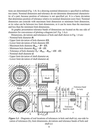
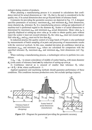
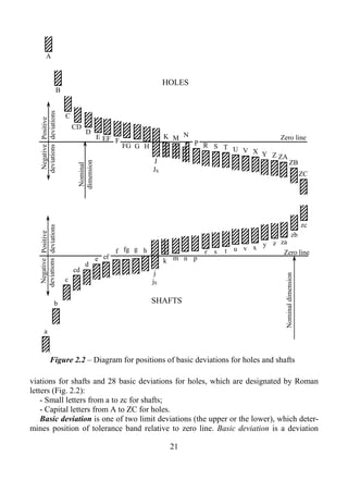
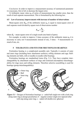
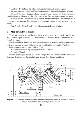
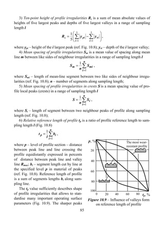
7 INTERCHANGEABILITY OF THREADED JOINTS
Threaded joints are widely applied in machine-building industry and in aeronautics
brunch (Fig. 7.1).
External
thread
Internal
thread
a b c
Figure 7.1 – Bolt (a), nut (b) and threaded joint (c)
46](https://image.slidesharecdn.com/basicsofinterchangeability-120508070541-phpapp02/85/Basics-of-interchangeability-46-320.jpg)


![List of literature used
1. Желєзна, А.М. Основи взаємозамінності, стандартизації та технічних вимірю-
вань [Текст]: навч. посіб. / А.М. Желєзна, В.А. Кирилович. – К.: Кондор, 2004.
– 796 с.
2. Единая система допусков и посадок СЭВ в машиностроении и приборострое-
нии: справочник: в 2 т. – 2-е изд., перераб. и доп. – М.: Изд-во стандартов,
1989. – Т. 1. – 263 с. – Т. 2. – 208 с.
3. Анухин, В.И. Допуски и посадки [Текст]: учеб. пособие. – 4-е изд. / В.И. Ану-
хин. – СПб.: Питер, 2007. – 207 с.
4. Якушев, А.И. Взаимозаменяемость, стандартизация и технические измерения
[Текст]: учеб. для втузов / А.И. Якушев, Л.Н. Воронцов, Н.М. Федотов. – 6-е
изд., перераб. и доп. – М.: Машиностроение, 1987. – 352 с.
5. Болдин, Л.А. Основы взаимозаменяемости и стандартизации в машинострое-
нии [Текст]: учеб. пособие для вузов / Л.А. Болдин. – 2-е изд., перераб. и доп.
– М.: Машиностроение, 1984. – 272 с.
89](https://image.slidesharecdn.com/basicsofinterchangeability-120508070541-phpapp02/85/Basics-of-interchangeability-89-320.jpg)