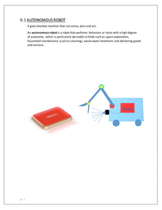
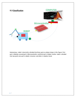
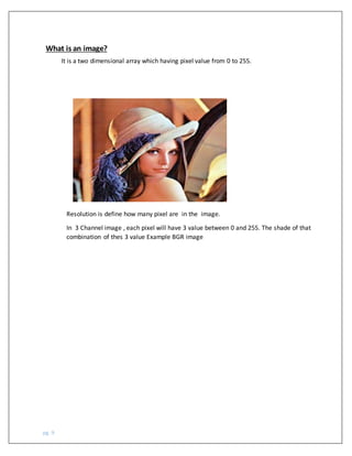
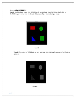
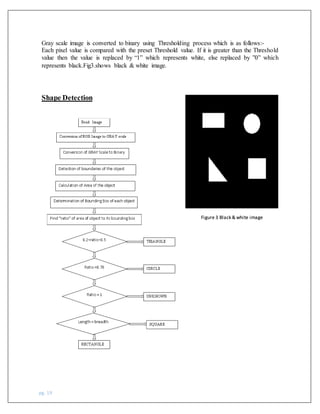
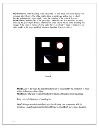
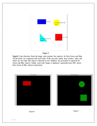
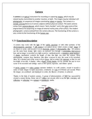
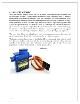
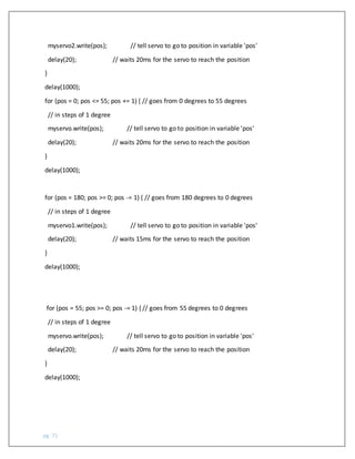
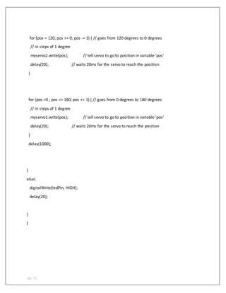
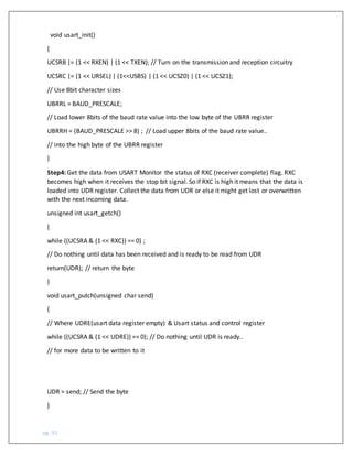
The document discusses an approach for identifying the work of an autonomous robot using image processing techniques, specifically employing MATLAB and microcontroller integration with Arduino for real-time applications. The paper covers various aspects of image processing such as color detection, shape recognition, and the use of serial communication to control robotic actions. Practical implications include automation in industries, enhancing efficiency, and reducing manual labor by performing tasks in challenging environments.
![pg. 8
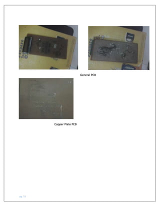
Matlab
MATLAB (matrix laboratory) is a multi-paradigm numerical computing environment
and fourth-generation programming language. A proprietary programming
language developed by MathWorks, MATLAB allows matrix manipulations, plotting
of functions and data, implementation of algorithms, creation of user interfaces, and
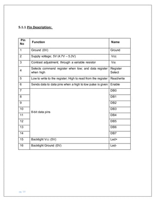
interfacing with programs written in other languages,
including C, C++, Java, Fortran and Python.
Although MATLAB is intended primarily for numerical computing, an optional toolbox uses
the MuPAD symbolic engine, allowing access to symbolic computing abilities. An
additional package, Simulink, adds graphical multi-domain simulation and model-based
design for dynamic and embedded systems.
This paper deals with the implementation of various MATLAB functions present in image
processing toolbox of MATLAB and using the same to create a basic image processor having
different features like, viewing the red, green and blue components of a color image separately,
color detection and various other features (noise addition and removal, edge detection,
cropping, resizing, rotation, histogram adjust, brightness control, etc.) that is used in a basic
image editor along with object detection and tracking.
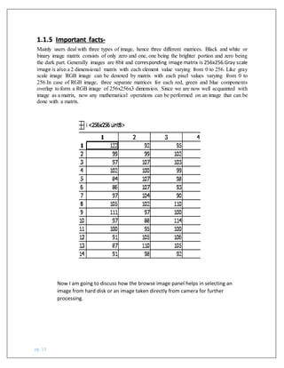
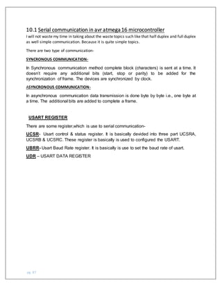
In Matlab we deal with the matrix and we know that the matrix is formed with the ROW and
Column element. Matlab very easily deal with Matrix. And we are seeing with example.
a= [1, 2, 3; 4, 7, 9; 9, 6, 5]
a =
1 2 3
4 7 9
9 6 5
>> a (2:3)=6
a =
1 2 3
6 7 9
6 6 5
>> a(2:3,2:3)=6
a =
1 2 3
6 6 6
6 6 6](https://image.slidesharecdn.com/autonomousrobot-210329065703/85/Autonomous-robot-8-320.jpg)
![pg. 16
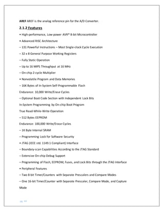
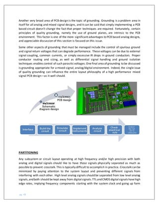
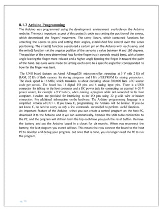
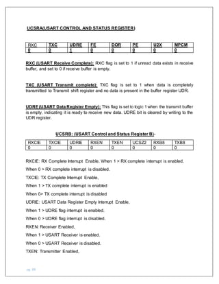
1.1.8 Noise AdditionandRemoval-
Various types of noise get added to an image when a snapshot is taken. In order to get
rid of these noises various types of filters are used. To illustrate this authors have added a noise
to an image externally and then applied various filters to get rid of it and evaluated the results.
Since noises are two dimensional and RGB images are three dimensional, dimensional
mismatch has to be avoided while adding the noises. For this reason
RGB image is converted to gray image and then noise addition and removal is performed.
When we talk about the noise in the image then noise is a also a great problem. It is unwanted
part in image.
Noisyimage
For removing noise we have to apply filter. Filter basicaly is used to remove the unwanted
part.
B=imopen(I,se);% these are only use to remove unwanted part
final= imclose(B,se);% it is also use to remove unwanted part or we can say it fill the part
which is unwanted or blank.
diff_im = medfilt2(diff_im, [3 3]);
%Use a median filter to filter out noise.
Here the medfilt2(,[]) use for removing noise. This command take the median of the element
of the matrix and other point ,what is dimensional you are taking. And this median value apply
for the all noise area or on the pixel.
In the above command we have taken [3X3] dimension, and this dimension will be applicable
for all the entire dimension of image, So we can remove the noise.](https://image.slidesharecdn.com/autonomousrobot-210329065703/85/Autonomous-robot-16-320.jpg)
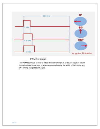
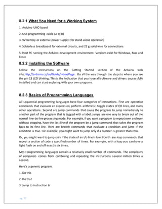
![pg. 23
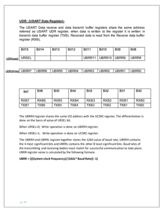
• clc; clear all; close all;
• s=imread('Image1.jpg');
• imshow(s);
• diff_im = imsubtract(s(:,:,1), rgb2gray(s));
• diff_im = medfilt2(diff_im, [8 8]);
• bw = im2bw(diff_im,0.18);
• figure, imshow(bw);
• [L,N] = bwlabel(bw, 8);
• pre=regionprops(L);% here Lcontains the matrix of diffrent pixelof & bw contains the
the number of blob.
• figure, imshow(bw);
• hold on
• for n=1:size(pre,1)
• rectangle('Position',pre(n).BoundingBox,'EdgeColor','r','LineWidth',2);
• End
This program is very helpful in finding the position of object.
Here one conflict occurs, how we can find the position of object in the image, in the
above discussion, I have discussed how we can find the color of object.
You have to follow all these step unless you get binary image and when you will have
the binary image then apply the “regionprops()” command ,this command basically
help us to find where the pixel intensity is greater than the 0 , as we know that if there
is different intensity of related pixel in gray scale image then we apply the one
command that is “bwlabel()” this command can help us, in order to find how many
different type of pixel are present and it contains the matrix for all the different pixel.
After applying the command, we can find the maximum and minimum value of the
row and column respectively. And with the help of it we can draw a bow around it.
1.1.12Howto plota box](https://image.slidesharecdn.com/autonomousrobot-210329065703/85/Autonomous-robot-23-320.jpg)
![pg. 25
Matlab has built-in adaptors to access the camera. At the Matlab command prompt, write
the ‘imaqhwinfo’ instruction and press ‘Enter’ key. This instruction returns information
about all the adaptors available in the system: ans = InstalledAdaptors:
{‘winvideo’}
MATLABVersion: ‘7.0.1 (R14SP1)’
ToolboxName: ‘Image Acquisition
Toolbox’
ToolboxVersion: ‘1.7 (R14SP1)’
The ‘info=imaqhwinfo’ instruction returns information about a specific device accessible
through a particular adaptor.
The output of the ‘info = imaqhwinfo(‘winvideo’)’ instruction is: info
=AdaptorDllName:G:MATLAB701toolboximaqimaqadaptorswin32
mwwinvideoimaq.dll’ AdaptorDllVersion: ‘1.7 (R14SP1)’
AdaptorName: ‘winvideo’
DeviceIDs: {1x0 cell}
DeviceInfo: [1x0 struct]
The output of the ‘dev_info = imaqhwinfo(‘winvideo’, 1)’ instruction is:
dev_info =
DefaultFormat: ‘RGB24_640x480’
DeviceFileSupported: 0
DeviceName: ‘WebCam Vista #2’
DeviceID: 1
ObjectConstructor:
‘videoinput(‘winvideo’, 1)’
SupportedFormats: {1x11 cell}
Again, the ‘obj = videoinput(‘adaptorname’, deviceID,’ format’)’ instruction constructs a
video input object where the ‘adaptorname’ string specifies the name of the device adaptor
that the object ‘obj’ is associated with. ‘deviceID’ is the identifier of the device in numerical
number. If ‘deviceID’ is not specified, the first available device ID is used. The ‘format’ string
specifies the video format for the object. If the format is not specified, the device default
format is used. For example, the output of the ‘obj= videoinput
(‘winvideo’, 1,’RGB24_640×480')’ instruction will be:
1.2.2 How to access camera in Matlab?](https://image.slidesharecdn.com/autonomousrobot-210329065703/85/Autonomous-robot-25-320.jpg)
![pg. 28
Spatial coordinates. Consider a pixel as a square patch. From this perspective, a location
such as (3.3, 2.2) is a spatial coordinate. Here, locations in an image on a plane are described
in terms of ‘x’ and ‘y.’ When the syntax uses ‘x’ and ‘y,’ it refers to the spatial coordinate
system. Fig. 2 shows the coordinate convention of the spatial coordinate system. Notice that
‘y’ increases downward. An image may be defined as a two dimensional f(x, y) function,
where ‘x’ and ‘y’ are spatial coordinates, and the amplitude of ‘f’ at any pair of coordinates
(x, y) is called the intensity or gray level of the image at the point. The finite discrete values
of the coordinates (x, y) and amplitude of ‘f’ are the digital images.
An intensity image is a data matrix whose values have been scaled to represent intensities.
When the elements of an intensity image are of class ‘uint8’or class ‘uint16,’ they have
integervaluesinthe range [0,255] and [0, 65535], respectively.The classof the elements used in
this program is ‘uint8.’](https://image.slidesharecdn.com/autonomousrobot-210329065703/85/Autonomous-robot-28-320.jpg)
![pg. 30
Se = strel (‘disk’, 20); % creates a flat, disk-shaped
structuring element with radius 20
B= imopen (I, se);
%morphological opening Final= imclose (B, se);
%morphological closing
Morphological opening removes those regions of an object which cannot contain the
structuring element, smoothest object contours, breaks thin connections and removes thin
protrusions. Morphological closing also tends to smooth the contours of objects besides
joining narrow breaks and filling long, thin gulfs and holes smaller than the structuring
element:
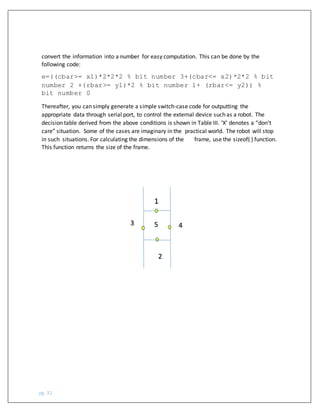
5. Once you obtain the desired part, find the Centre of the ball. The following statement
computes all the connected components in a binary image:
[L, n]= bwlabel(Final),
Here ‘n’ is the total number of connected components and ‘L’ is the label matrix. (Each
connected component is given a unique number.)
The following statement:
[r, c]= find (L= = K) % K= 1, 2 …n returns the row and column indices
for all pixels belonging to the Kth object:
rbar= mean (n);
cbar= mean(c);
Variables ‘rbar’ and ‘cbar’ are the coordinates of the Centre of mass. As you have already
filtered the image, the final image contains only one white region. But in case there is a
computational fault due to excessive noise, you might have two connected components. So
form a loop from ‘1’ to ‘n’ using ‘for’ statement, thus calculating the Centre of mass for all
objects. The syntax is:
for K=1:n
If there are no components in a frame, the control doesn’t enter the loop and ‘rbar’ and ‘cbar’
remain initialized to zero. For checking the output on the computer, use the following
instructions:
imshow (rgb_image);
hold on
plot (cbar, rbar, ‘marker’, ‘ * ’, ‘MarkerEdgeColor’, B );
These statements pop-up a window where a ‘blue’ mark is plotted on the detected Centre of
mass of the red ball. They have been commented out in the main program for testing.](https://image.slidesharecdn.com/autonomousrobot-210329065703/85/Autonomous-robot-30-320.jpg)
![pg. 38
1.3.6 Detectionof the color and performing task-(code)
clc;clear all; close all;
% Capture the video frames using the videoinput function
% You have to replace the resolution & your installed adaptor
name.
vid = videoinput('winvideo',1,'YUY2_320X240');
% Set the properties of the video object
set(vid, 'FramesPerTrigger', Inf);
set(vid, 'ReturnedColorspace', 'rgb')
vid.FrameGrabInterval = 5;
%start the video aquisition here
start(vid)
k=0;
z=1
s=serial('COM3','Baudrate',9600,'databits',8);
fopen(s);
% Set a loop that stop after 100 frames of aquisition
while(vid.FramesAcquired<=200)
% Get the snapshot of the current frame
data = getsnapshot(vid);
% Now to track red objects in real time
% we have to subtract the red component
% from the grayscale image to extract the red components
in the image.
diff_im = imsubtract(data(:,:,1), rgb2gray(data));
%Use a median filter to filter out noise
diff_im = medfilt2(diff_im, [3 3]);
% Convert the resulting grayscale image into a binary image.
diff_im = im2bw(diff_im,0.18);
% Remove all those pixels less than 300px
diff_im = bwareaopen(diff_im,200);
% Label all the connected components in the image.
bw = bwlabel(diff_im, 8);% here L contains the matrix of
diffrent pixel of & bw contains the the number of blob.
% Here we do the image blob analysis.
% We get a set of properties for each labeled region.
stats = regionprops(bw,'BoundingBox', 'Centroid');% here
stats tell about all the properties of the image.
% Display the image](https://image.slidesharecdn.com/autonomousrobot-210329065703/85/Autonomous-robot-38-320.jpg)
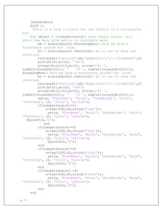
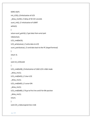
![pg. 89
When 1 >USART Transmitter is enabled.
When 0 > USART Transmitter is disabled.
iii. UCSRC: (USART Control and Status Register C)
The transmitter and receiver are configured with the same data features as
configured in this register for proper data
URSEL UMSEL UPM1 UPM0 USBS UCZ1 UCZ0 UCPOL
0 0 0 0 0 0 0 0
URSEL: USART Register select. This bit must be set due to sharing of I/O location by UBRRH and
UCSRC.
UMSEL: USART Mode Select,
When 1 > Synchronous Operation.
When 0 > Asynchronous Operation UPM [0:1]: USART Parity Mode, Parity mode selection bits.
USBS: USART Stop Select Bit, When 0>1 Stop Bit
When 1 >2 Stop Bits
UCSZ [0:1]: The UCSZ [1:0] bits combined with the UCSZ2 bit in UCSRB sets size of data frame
i.e., the number of data bits. The table shows the bit combinations with respective character
size
UCSZ2 UCSZ1 UCSZ0 Character size
0 0 0 5-bit
0 0 1 6-bit
0 1 0 7-bit
0 1 1 8-bit
1 0 0 Reserved
1 0 1 Reserved
1 1 0 Reserved
1 1 1 9-bit](https://image.slidesharecdn.com/autonomousrobot-210329065703/85/Autonomous-robot-89-320.jpg)
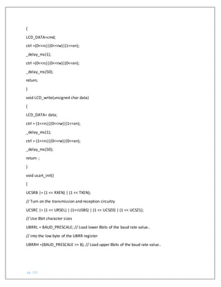


![[ PPT ] NS _ppt 4..ppt microprocesser and microcontroller fundamentals](https://cdn.slidesharecdn.com/ss_thumbnails/gurukulkangriuniversity-121014110754-phpapp02-thumbnail.jpg?width=640&height=640&fit=bounds)