Atoll 3.1.2 automatic cell planning module

© Forsk 2012 Slide 1Confidential – Do not share without prior permission
Automatic Cell Planning Module
Atoll 3.1.2

1. Introduction
2. Parameters Used by ACP
3. Network Reconfiguration Process
4. Site Selection Process
5. Other Topics
Training Programme

1. Introduction
Automatic optimisation tool for GSM, UMTS, CDMA, LTE and WIMAX networks
To improve existing networks by tuning parameters that can be easily changed remotely
• Antenna electrical tilt
• Power (BCCH for GSM, Pilot for UMTS, Reference Signal for LTE, Preamble for WiMAX)
To optimise a network still in the planning phase by:
• Selecting antennas
• Changing the antenna azimuth
• Changing the mechanical downtilt of the antenna
• Changing the antenna height
• Selecting sites among a list of candidate sites
Combined GSM/UMTS/LTE optimisation can be performed

1. Introduction
Principle
Optimisation of quality indicators
By automatic adjustments of network parameters
• Power (BCCH for GSM, Pilot for UMTS/CDMA, RS for LTE and Preamble for WiMAX)
• Antenna parameters:
• Type of antenna
• Azimuth
• Mechanical downtilt
• Electrical downtilt
• Height
GSM
• BCCH coverage
• Dominance of Best Server
UMTS/CDMA
• RSCP (Pilot) coverage
• CPICH Ec/Io
LTE
• Reference Signal coverage
• Reference Signal CINR
WIMAX
• Preamble coverage
• Preamble CINR

1. Introduction
Principle
Optimisation process based on a cost function
The cost function depends on quality figures
• In GSM: the cost decreases when the BCCH coverage and the Best Server’s dominance increase
• In UMTS/CDMA: the cost decreases when the Pilot coverage and Pilot quality increase
• In LTE: the cost decreases when the RS coverage and RS CINR increase
• In WIMAX: the cost decreases when the Preamble coverage and Preamble CINR increase
Iterative algorithm is used
• Each iteration corresponds to one network parameter change
• Then, changes are ranked from the change with the most benefit to the change with the least benefit

1. Introduction
5. Other Topics
Training Programme

2. Parameters used by ACP
Requirements
Existing and valid path loss matrices
Recommendations
Creating a Computation Zone
• Used to define the default area where
the ACP calculates statistics on
performance indicators
Creating a Focus Zone
• Used to define the default area in which
are the cells to be optimised
Computation zone
= Zone used to compute statistics on
performance indicators (by default)
Focus zone
= Area where the optimisation will
be performed (by default)

1. Introduction
5. Other Topics
Training Programme

Creating an Optimisation Setup
Defining Optimisation Parameters and Objectives
Running an Optimisation Process
Viewing Optimisation Results
Analysing Optimisation Results

Creating an Optimisation Setup
To run the optimisation
immediately
To save the defined optimisation
parameters and run the optimisation later

Defining Optimisation Parameters (1/9)
Selection of layers to be optimised
Layer(s) configuration
Several in case of Multi-RAT
networks (GSM+UMTS+LTE)

Selection of zones to be optimised
Zones definition
Possibility to define
zones to be specifically
optimized, using:
• Clutter Classes,
• Hot Spots zones,
• .shp files

Choice between quality or financial cost based optimisation
No cost control: the optimisation is only
based on quality
 Useful when planning a new network
Possibility to limit the financial cost of the
optimisation:
• Maximum financial cost allowed
• Compromise between the financial cost
and the quality
 Useful when improving an existing
network
Definition of the financial cost for:
• Each parameter change
• Each site visit
• etc...

Selection of transmitters/cells to be optimised
Definition of parameters that can be modified by ACP
To define Cells’ Optimisation parameters
(Subcells power in GSM, Pilot power in UMTS, RS power in
LTE and Preamble power in WiMAX)

By default, GSM-UMTS-LTE transmitters sharing the same antenna parameters are linked
An auto-Link function based on site coordinates, antenna height, azimuth and mechanical tilt is provided

Definition of Antenna Groups
To give some directives when reconfiguring the antenna type or the electrical tilt
Multi band “Physical Antenna”
Dual 900 1800 – 65deg17dBi
Multi band “Physical Antenna”
Dual 900 1800 – 36deg20dBi
Antenna Element
65deg17dBi@900
Antenna Element
65deg17dBi@1800

Step 1 : Create “Antenna Element” (using radiating patterns)
• An “Antenna Element” is
defined by one gain, one
beamwidth and one frequency
band
• For a given frequency band, a
given beamwidth and a given
gain, the “Antenna element” is a
group of antenna patterns
obtained with different electrical
tilt values
Antenna patterns table

Step 2 : Create “Physical Antennas” (using Antenna Elements)
To define multiband antennas
Multi band
“Physical
Antenna”
Antenna Elements

Step 3 : Create “Antenna Groups” (using Physical Antennas)
To define groups of Physical Antennas that will be then assigned to transmitters in the reconfiguration tab
Antenna groups to be
assigned to TXs in the
Reconfiguration tab
Created Physical Antennas

Defining Objectives (1/11)
ACP allows you to define Quality and Coverage objectives for each technology
Objectives are assessed over a “Target Zone” (Computation Zone, by default)
Objectives defined by the user Indicators to be optimized

Objective & Zone weighting
Objectives and Zones can be weighted according to their relative importance
Give priorities to specific Zones *
(* Priorities only apply if the “Zone Weighting” option is checked)
Give a priority to each objective

Traffic weighting (per objective)
ACP is able to focus more specifically on areas with a high traffic
Default option: NONE
the traffic is assumed to be uniform
 The quality indicator measured on
each pixel has the same weight
Selection of traffic maps (non-uniform traffic) to weight map pixels
 The quality indicators measured on each pixel can be weighted
by using the traffic density on that pixel

Example: Defining UMTS objectives
Coverage objectives : UMTS RSCP Coverage
Define the
Minimum Pilot
Signal Level to
get on each
pixel of the
“Target Zone”
Coverage to be
respected while
meeting the
RSCP coverage
conditions

Quality objectives : UMTS EcIo
Define the
Minimum Pilot
Quality to get
on each pixel
of the “Target
Zone”
Coverage to be
respected while
meeting the Pilot
Quality
conditions

UMTS Objectives Parameters
For each indicator to optimize, ACP settings (display configuration, shadowing margin…) can be:
• Either, taken from an existing prediction
• Or, defined manually

Summary of the indicators that can be optimized for each technology
GSM
•BCCH coverage
•Dominance of Best
Server
(= Number of potential
servers must be < 4)
UMTS/CDMA
•RSCP (Pilot) coverage
•CPICH Ec/Io
•Pilot Pollution
(= Number of cells in the
Active Set > 3)
LTE
•Reference Signal
coverage (or RSRP)
•Reference Signal CINR
(or RS C/N, RSRQ)
•Overlap
(= Number of potential
servers must be < 4)
WIMAX
•Preamble coverage
•Preamble CINR
•Overlap

Load balancing (Optional)
ACP enables you to create and manage capacity planning objectives
• To prevent load imbalance between sectors and thus avoid the degradation of some KPIs
Example: Optimisation of a UMTS network by ACP without Load Balancing
The Load balancing feature relies on 2 performance indicators:
• The “Average Load” improvement (%), measures how the average load improves from the initial value
• The “Load Balance” (%), measures the dispersion of cells loads
Cell A: Up-tilt (2°)
Cell B: Down-tilt (1°)
• Traffic served
• Cell load
- DL Total Power
- UL Noise Rise
• Interference
• Risk of congestion
Cell Load A = 75% ; Cell Load B = 60%
Solution: Load Balancing !
Cell A Cell A
Cell B Cell B
Cell Load A = 98% ; Cell Load B = 45%
(Statistics on Cell A)

Can be activated in the “Objectives” tab under “Load Balancing”
Recommendation:
Keep the default
configuration
Allows you to select the
layers for which load
balancing is performed

Traffic related to capacity planning can be defined in the “Capacity” tab
Traffic can be
considered as uniform
(evenly spread on each
service area) or,
generated from traffic
maps

ACP is designed to perform load balancing across multiple layers and technologies
For each service used,
traffic is balanced across
all the available layers
and technologies
For each service and
each technology, define
the minimum quality
required by a cell to
provide the service
To increase traffic density
specifically on some
zones. Traffic is scaled
according to the weights
defined in the “Zone
Weighting” tab.

Running an Optimisation Process (1/4)
Graphical display of the optimisation progress
“Graphs” tab: Variation of performance objectives in real time with iterations
The optimisation process can be
paused or stopped early

“Changes” tab: Type and number of changes

“Quality” tab: Coverage and Quality improvements (variations)

“Objectives” tab: To see at a glance if the objective is achieved or not
Select the
objective to be
analysed
(coverage and
quality
indicators)

Viewing Optimisation Results (1/5)
Optimisation results are stored in the optimisation
folder
Results available in 7 tabs
“Statistics” tab: synthesised view of optimisation
results for each objective
Statistics provided for the “Target zone”
• To get statistics on the other zones select “Show
Detailed Zone Results”
Statistics
for each
objective
Global report available
in “Excel” format

“Graph” and “Quality” tabs
Histogram displaying statistics within the
computation zone or the focus zone
Coverage and Quality maps
before and after the optimisation

“Capacity” tab
Provides capacity load statistics for the initial and the optimised network
The graph shows the ratio of cells
with a capacity load that is smaller
than a given capacity load value (%).
Usually, the best result that you can
get is a final curve (blue curve) on
top of the initial curve (red curve).
Statistics based on the values
displayed in the table (on the right)

“Change Details” tab
Analysis of improvements according to the number of changes
Changes are ordered by “profitability”
• The most “profitable” changes will be applied first
Slider to select a subset of all
changes and view the corresponding
performance improvement on the
graph (global improvement and
improvement of each objective)
List of changes ranked from the change
with the most effect to the change with
the least effect
Selected changes are displayed in green

“Commit” tab
To commit changes that you allowed in the “Change Details” tab
Transmitters/cells with
parameter changes are
displayed in green
Initial and final cell
parameters displayed
Revert the network to its state
before the optimisation was run
Apply the set of selected
changes

Analysing Optimisation Results (1/5)
Process
Quick validation of optimisation results using the ACP maps
• First analysis available without having to commit ACP results
• Based on the entire set of proposed changes
Deeper analysis with coverage predictions available in the predictions folder
• After committing ACP results
ACP Maps Available
Quality analysis maps
• Display of Coverage and Quality maps
Coverage analysis
• Status of the coverage according to the defined objectives used in the optimisation
Change analysis
• Analysis of changes: antenna, tilt, azimuth
Best server analysis
• Absolute values of changed parameters

Analysis with ACP Maps
ACP maps are automatically
calculated and inserted into
the folder containing the
optimisation results

Tiptext available for any ACP map
• The exact calculated value is displayed on each pixel
Display properties of ACP maps
• Automatic update of the ACP map after changing colours or range of values

Histogram available on ACP maps
Comparison tool
• Available to compare ACP maps from the same optimisation or from a different optimisation

Analysis with coverage predictions from the predictions folder
Requirement: Commit results of the optimisation
Calculating prediction studies before and after the optimisation
Generating reports on the predictions studies before and after the optimisation in order to check if
network quality figures have been improved
Possibility to “Roll back to Initial State”

1. Introduction
5. Other Topics
Training Programme

Overview
Defining Candidate Sites
Viewing Optimisation Results

Overview (1/2)
Examples of Site Selection process
Scenario 1: using ACP to select the best site among several candidates on a given geographical area
• 3 candidate sites available
• Candidate sites are assigned to a group where the minimum and the maximum site occurrence is set to “1”
 Among the 3 candidates, the ACP is forced to select only one site
Scenario 2: using ACP to deploy the LTE technology on a given area using existing UMTS sites
• About 40 UMTS sites (i.e. 40 candidate sites) available on the target area
• Candidate sites are assigned to a group where the minimum site occurrence is set to “10” and the maximum
to “20”
 Among the 40 candidates, the ACP is forced to select between 10 and 20 sites to reach objectives

Overview (2/2)
General process similar to the site reconfiguration process:
Creating an optimisation setup
Defining “Candidate” sites
Defining objectives and parameters to be optimised
• Note: The “Reconfiguration” mode is available (not mandatory) during the Site Selection process.
Running an optimisation process
Viewing optimisation results
Analysing optimisation results

Defining Candidate Sites (1/3)
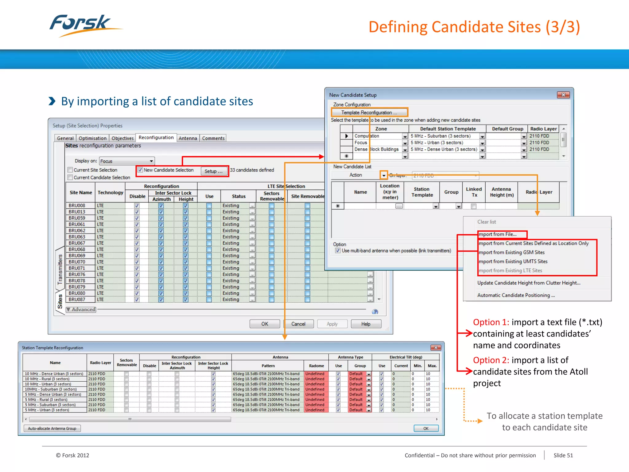
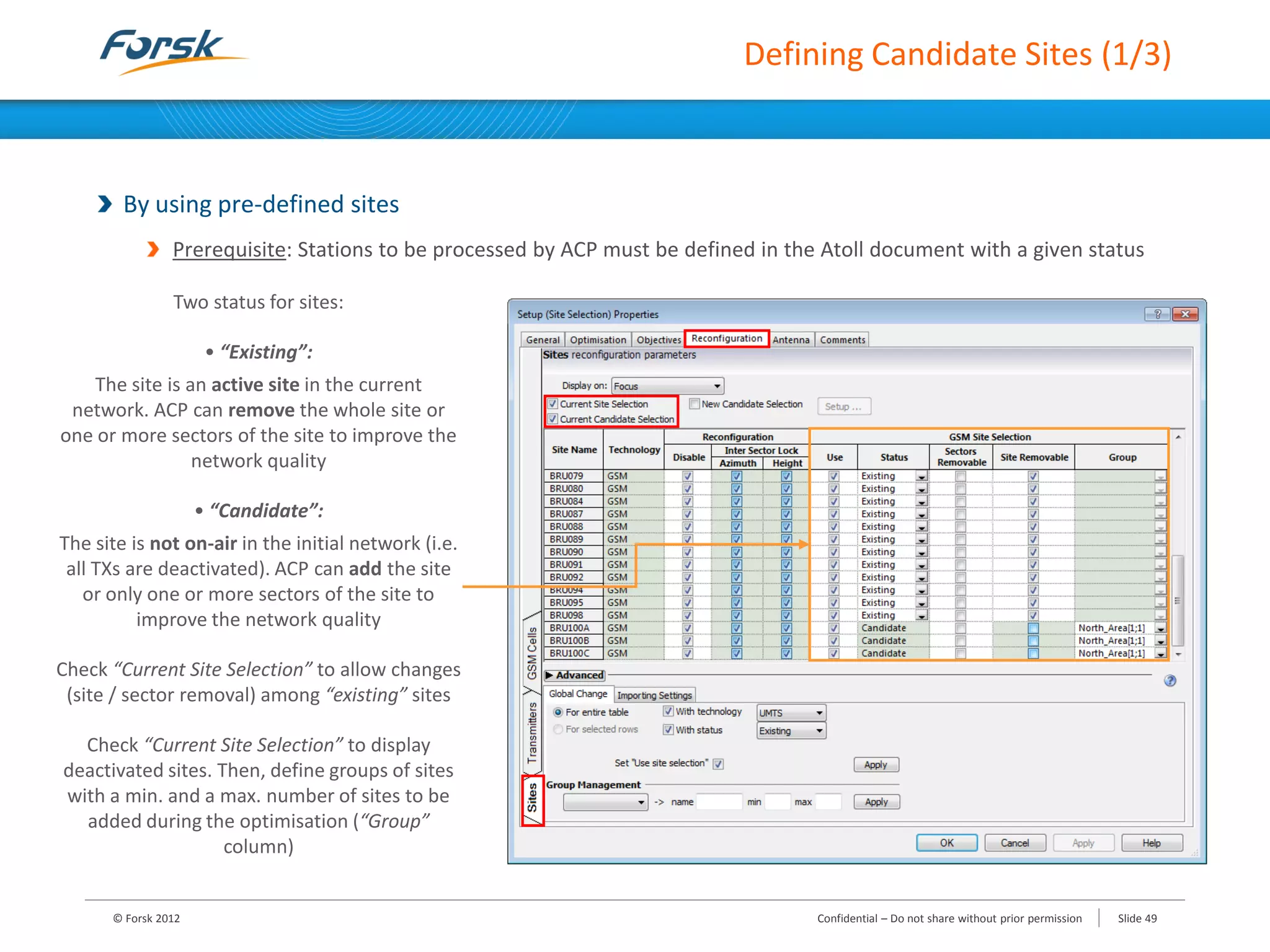
By using pre-defined sites
Prerequisite: Stations to be processed by ACP must be defined in the Atoll document with a given status
Two status for sites:
• “Existing”:
The site is an active site in the current
network. ACP can remove the whole site or
one or more sectors of the site to improve the
network quality
• “Candidate”:
The site is not on-air in the initial network (i.e.
all TXs are deactivated). ACP can add the site
or only one or more sectors of the site to
improve the network quality
Check “Current Site Selection” to allow changes
(site / sector removal) among “existing” sites
Check “Current Site Selection” to display
deactivated sites. Then, define groups of sites
with a min. and a max. number of sites to be
added during the optimisation (“Group”
column)

By using pre-defined sites
“Advanced” tab:
Allows you to apply the same
locking options to a set of sites,
and to manage groups
“Reconfiguration” column:
Select “Disable” to prevent ACP from making
any changes to the Transmitters or to the Cells,
as defined in the Transmitters and the
[Technology] Cells tabs
In case of network reconfiguration, you can
preserve the current angular separation
between antennas, and the relative height
difference between them

By importing a list of candidate sites
Option 1: import a text file (*.txt)
containing at least candidates’
name and coordinates
Option 2: import a list of
candidate sites from the Atoll
project
To allocate a station template
to each candidate site

Viewing Site Selection Results (1/3)
Statistics Report
Statistics and status of the
optimisation (Achieved or
Failed) for each objective
Select “Show Change Statistics” to get
statistics on the sites/sectors added or
removed, and all the changes made
during the optimisation process

Implementation Plan Analysis
Sites/TXs/Cells added or removed
List of changes (antennas, tilts, etc.)
if “Reconfiguration” mode selected

Transmitters/Cells Modifications Analysis
List of candidate TXs/cells to be
added
List of TXs/cells to be removed
List of changes (antennas, tilts,
etc.), if “Reconfiguration” mode
selected

1. Introduction
5. Other Topics
Training Programme

6. Other Topics
Combined GSM/UMTS/LTE Optimisation (in case of several .atl documents)
Data Loading and Validity Control
Saving Settings to Configuration Files
Configuring Default Settings

Combined GSM/UMTS/LTE Optimisation (1/2)
Requirements (in case of several .atl documents)
Several Atoll projects (GSM, UMTS and/or LTE .atl files) that must be opened in the same Atoll session
General process similar to a classic optimisation
Creating the optimisation setup
Defining optimisation parameters
Running the optimisation process
Viewing optimisation results
Analysing optimisation results

Combined GSM/UMTS/LTE Optimisation (2/2)
Procedure (in case of several .atl documents)
Step 1: Create the optimisation setup in one single technology document (a LTE document for ex.)
Step 2: Import other(s) network(s)’ configuration by importing associated project(s)

Data Loading and Validity Control (1/2)
Data used when running an optimisation process
Radio data (antennas, sites, transmitters)
Traffic parameters (services, terminals, etc.)
Geographic maps (DTM, clutter class and clutter height maps)
Traffic maps
Path loss matrices
Loaded when creating an
optimisation setup
Direct access when running the
optimisation process

Data Loading and Validity Control (2/2)
Data validity control when running an optimisation process
Atoll checks the consistency between the optimisation setup, the actual state of the network and path loss
matrices
If inconsistencies => existing optimisation setups are locked and new optimisation process cannot be run
Incoherence with existing setup when:
Data changes are performed after creating the setup (e.g. New transmitter, transmitter deactivated,
different transmitter settings, etc.)
Optimisation results have been committed
Path loss matrices are missing or not valid

Saving Settings to Configuration Files
Save or load a given Setup Configuration
Optimisation settings saved in a .PRJ file
(objectives per clutter class, lists of cells
to be reconfigured, reconfiguration
settings, etc.)
Import the configuration file containing
optimisation settings
Used to apply the same settings when
you create a new optimisation setup

Configuring User Preferences
Trade-off between
speed and quality
Enables you to activate
the “Multi-Storey” and
the “EMF Exposure”
extensions

Setup Template Configuration
Define default values of the
Optimisation Setup

Configuring Path Loss Matrices Storage
Define the folder to be
used by ACP to store
Path Loss Matrices
(used in case of Antenna
Height optimisation)

Thank you

Atoll 3.1.2 automatic cell planning module

More Related Content

What's hot

Similar to Atoll 3.1.2 automatic cell planning module

Recently uploaded

Atoll 3.1.2 automatic cell planning module