This document discusses the concept of asymmetric information in markets. It begins by defining asymmetric information as when one party in a market has more or better information than the other. It then provides examples of markets with asymmetric information such as medical services, insurance, and used cars.
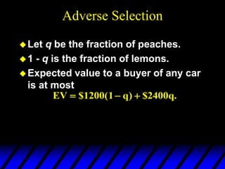
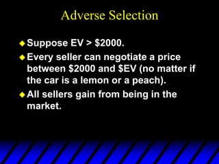
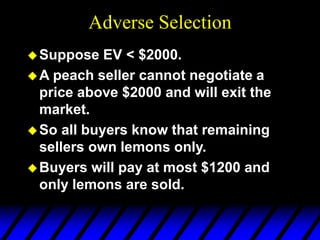
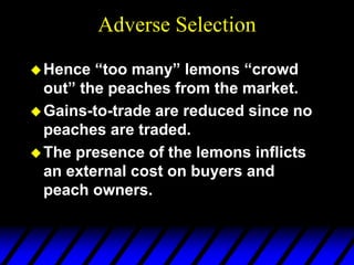
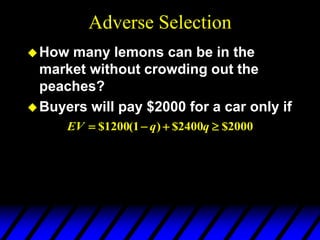
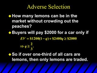
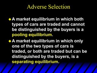
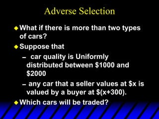
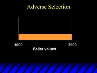
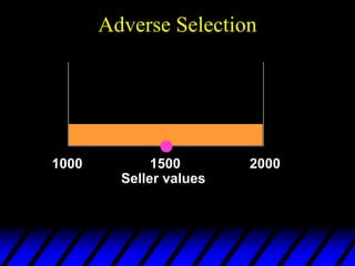
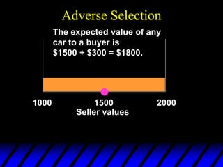
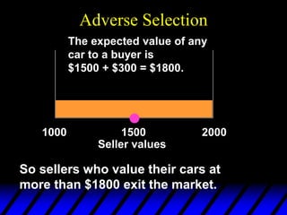
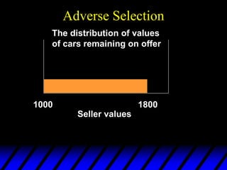
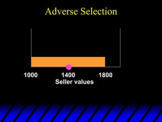
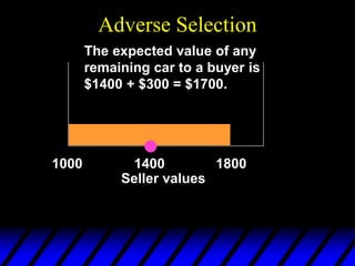
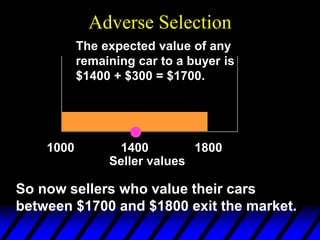
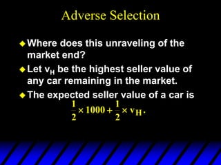
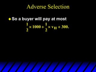
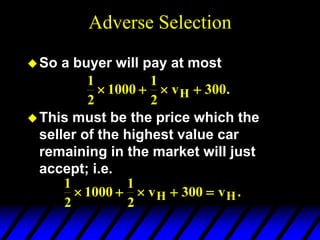
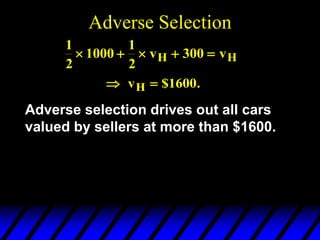
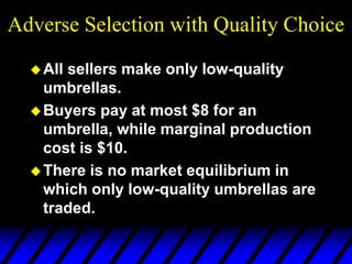
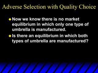
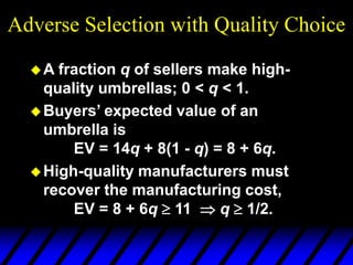
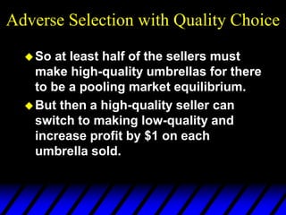
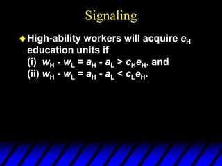
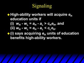
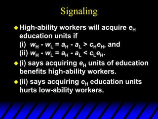
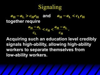
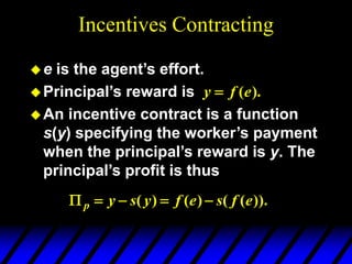
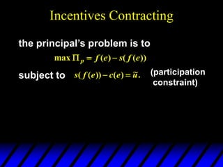
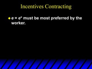
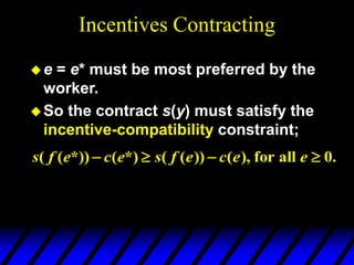
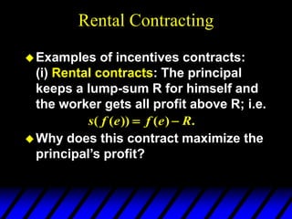
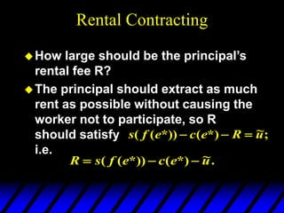
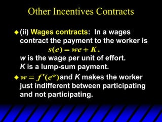
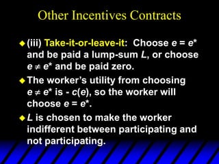
The document goes on to discuss how asymmetric information can negatively impact market functioning through concepts like adverse selection, signaling, moral hazard, and incentives contracting. Specifically, it provides detailed examples of how adverse selection in used car and umbrella markets can lead to market unraveling. It also discusses how signaling through education can help mitigate adverse selection but does not necessarily improve market efficiency. Finally, it briefly outlines how moral hazard and incentives contracting relate to asymmetric information problems.


![TRABAJO_DE_INVEST___VARIABLE_EL_CREDITO__Walter__7_(3)[1].pptx](https://cdn.slidesharecdn.com/ss_thumbnails/trabajodeinvestvariableelcreditowalter731-250108204036-1f8edab7-thumbnail.jpg?width=640&height=640&fit=bounds)


