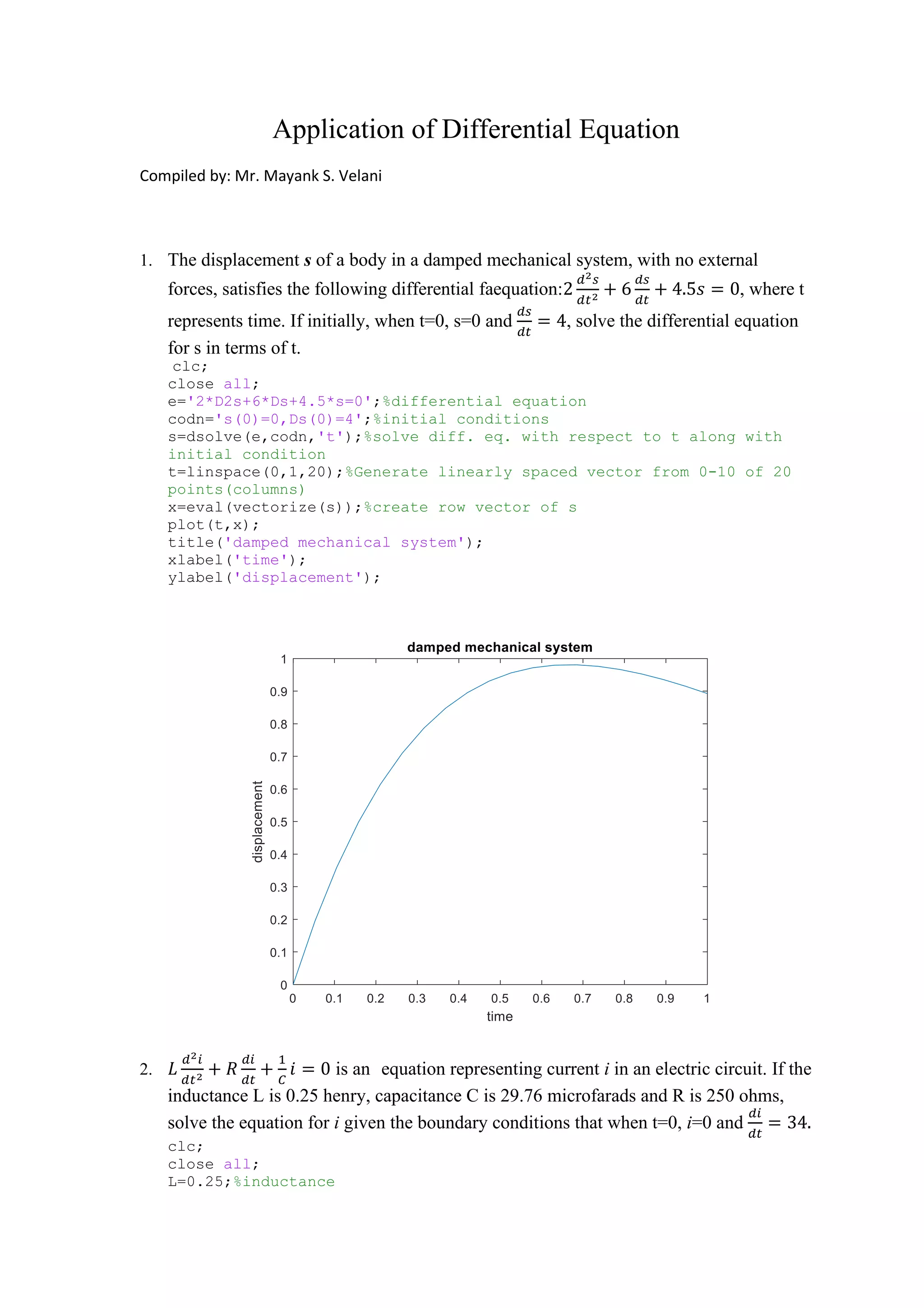
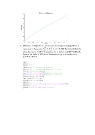
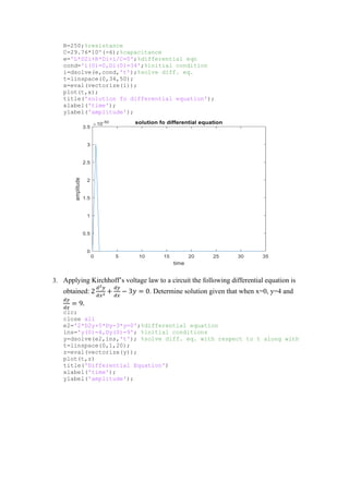
1. The displacement s of a damped mechanical system satisfies a differential equation with initial conditions of s=0 and ds/dt=4. The equation is solved for s in terms of time t. 2. A differential equation representing current i in an electric circuit is solved given initial conditions when t=0 of i=0 and di/dt=34. 3. A differential equation obtained from applying Kirchhoff's voltage law to a circuit is solved given initial conditions of y=4 and dy/dx=9 when x=0.

1. Application of Differential Equation
Compiled by: Mr. Mayank S. Velani
1. The displacement s of a body in a damped mechanical system, with no external
forces, satisfies the following differential faequation:2
𝑑2𝑠
𝑑𝑡2
+ 6
𝑑𝑠
𝑑𝑡
+ 4.5𝑠 = 0, where t
represents time. If initially, when t=0, s=0 and
𝑑𝑠
𝑑𝑡
= 4, solve the differential equation
for s in terms of t.
clc;
close all;
e='2*D2s+6*Ds+4.5*s=0';%differential equation
codn='s(0)=0,Ds(0)=4';%initial conditions
s=dsolve(e,codn,'t');%solve diff. eq. with respect to t along with
initial condition
t=linspace(0,1,20);%Generate linearly spaced vector from 0-10 of 20
points(columns)
x=eval(vectorize(s));%create row vector of s
plot(t,x);
title('damped mechanical system');
xlabel('time');
ylabel('displacement');
2. 𝐿
𝑑2𝑖
𝑑𝑡2
+ 𝑅
𝑑𝑖
𝑑𝑡
+
1
𝐶
𝑖 = 0 is an equation representing current i in an electric circuit. If the
inductance L is 0.25 henry, capacitance C is 29.76 microfarads and R is 250 ohms,
solve the equation for i given the boundary conditions that when t=0, i=0 and
𝑑𝑖
𝑑𝑡
= 34.
clc;
close all;
L=0.25;%inductance

2. R=250;%resistance
C=29.76*10^(-6);%capacitance
e='L*D2i+R*Di+i/C=0';%differential eqn
cond='i(0)=0,Di(0)=34';%initial condition
i=dsolve(e,cond,'t');%solve diff. eq.
t=linspace(0,34,50);
x=eval(vectorize(i));
plot(t,x);
title('solution fo differential equation');
xlabel('time');
ylabel('amplitude');
3. Applying Kirchhoff’s voltage law to a circuit the following differential equation is
obtained: 2
𝑑2𝑦
𝑑𝑥2
+
𝑑𝑦
𝑑𝑥
− 3𝑦 = 0. Determine solution given that when x=0, y=4 and
𝑑𝑦
𝑑𝑥
= 9.
clc;
close all
e2='2*D2y+5*Dy-3*y=0';%differential equation
ins='y(0)=4,Dy(0)=9'; %initial conditions
y=dsolve(e2,ins,'t'); %solve diff. eq. with respect to t along with
t=linspace(0,1,20);
z=eval(vectorize(y));
plot(t,z)
title('Differential Equation')
xlabel('time');
ylabel('amplitude');

3. 1. The motion of the pointer of a galvanometer about its position of equilibrium is
represented by the equation 𝐼
𝑑2𝑦
𝑑𝑥2
+ 𝐾
𝑑𝑦
𝑑𝑥
+ 𝐹𝑦 = 0. If I, the moment of inertia
about the pivot is 5x10−3
, K resistance due to friction is 2x10−2
and the F,
force on the spring is 0.20, solve the equation for y in terms of t when
y(0)=0.3, y’(0)= 0.
clc;
clear all;
close all;
I=5*10^(-3);%inertia of pointer
k=2*10^(-2);%resistance due to friction
F=0.02;%force on spring
eqn='I*D2y+k*Dy+F*y=0';%motion of pointer
ins='y(0)=0.3,Dy(0)=0';%initial condition
y=dsolve(eqn,ins,'t');
t=linspace(0,10,20);
z=eval(vectorize(y));
plot(t,z);
title('motion of the pointer of galvanometer');
xlabel('time');
ylabel('angular velocity theta');

4. 2. According to drag equation, the velocity of an object moving through a fluid
can be modeled by the equation
𝑑𝑢
𝑑𝑥
= −𝑘𝑢2
where k is a constant and k=0.82
and u(0)=40.
clc;
close all
e2='Du+0.82*u^2=0';%drag eqn
ins='u(0)=40';%initial velocity
u=dsolve(e2,ins,'t');
t=linspace(0,1,20);
z=eval(vectorize(u));
plot(t,z)
title('velocity of an object moving through a fluid ')
xlabel('time');
ylabel('Velocity');

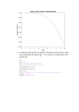
5. 3. Glucose is added intravenously to the blood stream at the rate of q units per minute and
the body removes glucose from the blood stream at the rate proportional to the amount
present. Assume A is the amount of glucose in the blood stream at time t and that the
rate of change amount of glucose is
𝑑𝑦
𝑑𝑥
= 𝑞 − 𝑘𝑦. Initial condition y(0)=0 and assume
k=0.1 and q=0.05.
clc;
clear all;
close all;
tspan=[0 10];%time interval
y0=0;%amount of glucose at initial
q=0.05;
k=0.1;
[t,y]=ode45(@(t,y)q-k*y,tspan,y0);%rate of change of amount of
glucose
plot(t,y);
title('glucose in blood stream');
xlabel('time(minutes)');
ylabel('amount of glucose');

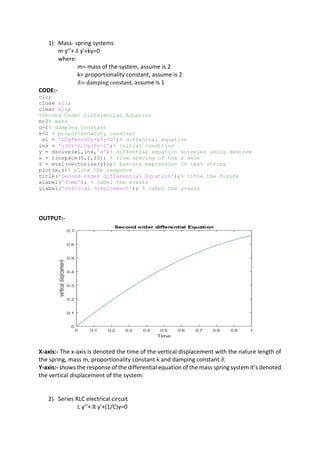
6. 4. A corporation invests part of its receipts at a rate of y=5500 rupees per year in a fund
for future corporate expansion. The fund earns 2 percent interest per year compounded
continuously. The rate of growth of the amount y in the fund is
𝑑𝑦
𝑑𝑥
= 𝑟𝑦 − 𝑝 . Solve
the differential equation for y as a function of time where y=0 at t=0.
clc;
clear all;
close all;
tspan=[0 4];%time interval
y0=0;%initial investment
p=5500;%amount
r=2;%interest per year
[t,y]=ode45(@(t,y)r*y+p,tspan,y0);%rate of growth of amount
plot(t,y);
title('Growth of investment');
xlabel('time(years)');
ylabel('Amount(Rupees)');

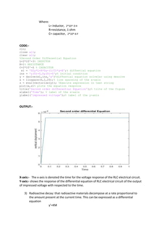
7. 5. The limiting capacity of the habitat of a wildlife herd is 750. The growth of the habitat
is
𝑑𝑦
𝑑𝑥
is proportional to the unutilized opportunity for growth as described by the
differential equation
𝑑𝑦
𝑑𝑥
= 𝑘(750 − 𝑦). When t=0, the population of the heard is 100
and k=0.8. Find the population heard over 4 years.
clc;
clear all;
close all;
tspan=[0 4];%time interval
k=0.8;
y0=100;%initial population
[t,y]=ode113(@(t,y)k*(750-y),tspan,y0);%rate of gwoth of
wildlife herd
plot(t,y);
title('Population of wildlife herd');
xlabel('time(years)');
ylabel('Population');

8. 6. An apple pie with an initial temperature of 170 ℃ is removed from the oven and
left to cool in the room with an air temperature of 20℃. Given that temperature
of pie initially decreases at the rate of 3 ℃/min . obtain the rate of cooling with
respect to t. Assume Newton’s law of cooling. Assume k=0.2.
𝑑𝑦
𝑑𝑥
= −𝑘(𝑦 − 20), 𝑦(0) = 170; 𝑦(0) = −3
clc;
clear all;
close all;
tspan=[0 15];%time interval
k=0.2;
y0=170;%initial teperature
[t,y]=ode45(@(t,y)-k*y+20*k,tspan,y0);%newton's law of cooling
plot(t,y);
title('Newton Law of cooling');
xlabel('time');
ylabel('temperature');

9. 1) Mass- spring systems
m y’’+ 𝛿 y'+ky=0
where:
m= mass of the system, assume is 2
k= proportionality constant, assume is 2
𝛿= damping constant, assume is 1
CODE:-
clc;
close all;
clear all;
%Second Order Differential Equation
m=2% mass
u=1% damping constant
k=2 % proportionality constant
e1 = 'D2y*m+u*Dy+k*y=0';% diffential equation
ins = 'y(0)=0,Dy(0)=1';% initial condition
y = dsolve(e1,ins,'x')% diffential equation solveler using desolve
x = linspace(0,1,20); % line spacing of the x axis
z = eval(vectorize(y));% Execute expression in text string
plot(x,z)% plote the responce
title('Second order differential Equation');% title the figure
xlabel('Time'); % label the x-axis
ylabel('vertical displcement'); % label the y-axis
OUTPUT:-
X-axis:- The x-axis is denoted the time of the vertical displacement with the nature length of
the spring, mass m, proportionality constant k and damping constant 𝛿.
Y-axis:- shows the response of the differential equation of the mass spring system it’s denoted
the vertical displacement of the system.
2) Series RLC electrical circuit
L y’’+ R y'+(1/C)y=0

10. Where:
L= inductor, 2*10^-3 H
R=resistance, 1 ohm
C= capacitor, 2*10^-6 F
CODE:-
clc;
close all;
clear all;
%Second Order Differential Equation
L=2*10^-3% INDUCTOR
R=1% RESISTANCE
C=2*10^-6 % CAPACITOR
e1 = 'D2y*L+R*Dy+(1/C)*y=E';% diffential equation
ins = 'y(0)=0,Dy(0)=0';% initial condition
y = dsolve(e1,ins,'x')%diffential equation solveler using desolve
x = linspace(0,1,20);% line spaceing of the x-axis
z = eval(vectorize(y)); %Execute expression in text string
plot(x,z)% plote the equation responce
title('Second order differential Equation');% tilte of the figure
xlabel('Time'); % label of the x-axis
ylabel('impressed voltage');% label of the y-axis
OUTPUT:-
X-axis:- The x-axis is denoted the time for the voltage response of the RLC electrical circuit.
Y-axis:- shows the response of the differential equation of RLC electrical circuit of the output
of impressed voltage with respected to the time.
3) Radioactive decay: that radioactive materials decompose at a rate proportional to
the amount present at the current time. This can be expressed as a differential
equation
y’=KM

11. Where:
M=mass of radioactive material
K= constant
CODE:-
clc;
close all;
clear all;
%First Order Differential Equation_1
k=1;% constant
e1 = 'Dy=k*y'; %differential equation
cond = 'y(0)=1';% initial condition
y = dsolve(e1,cond,'x')%diffential equation solveler using desolve
x = linspace(0,1,20); % line spacing of the x-axis
z = eval(vectorize(y));%Execute expression in text string
plot(x,z)% plot the responce of the equation
title('First order differential Equation_1'); % title of the figure
xlabel('Time'); % label of the x-axis
ylabel('material decompose rate'); % label of the y-axis
OUTPUT:-
X-axis:- The x-axis is denoted the time for the decomposition of the radioactive material time
for the decomposition rate.
Y-axis:- shows the response of the differential equation at different values for the
decomposition rate with respect to time.
4) Stephen howking discover that black holes emit a small amount of radiation, causing
them to slowly evaporate over time. According to hawking, the mass M of a black hole
obeys the differential equation.
y’= -(k/y^2)
Where k= 1.26*10^23 Kg/year

12. CODE:-
close all;
clear all;
%First Order Differential Equation_1
k=1.26*10^23;% constant
e1 = 'Dy=-(k/y^2)';% diffrential equation
cond = 'y(0)=1'; % initial condition
y = dsolve(e1,cond,'x')%diffential equation solveler using desolve
x = linspace(0,1,20);% line spaceing of the x-axis
z = eval(vectorize(y));%Execute expression in text string
plot(x,z)% plot the responce of equation
title('First order differential Equation_1');% title of the figure
xlabel('year'); % label of the x-axis
ylabel('Radiation');% label of the y-axis
OUTPUT:-
X-axis:- Rang of x-axis is multiplying factor of the year the x-axis denoted the year with respect
to emit the radiation by black hole.
Y-axis:- shows the response of the differential equation the differential equation is denotes
the rate of the emit radiation with respect to year.
5) According to the drag equation the velocity of an object moving through a fluid can
be modelled by the equation.
y’= -k*y^2
Assume initial velocity =30 m/sec

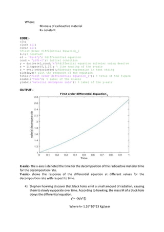
13. CODE:-
close all;
clear all;
%First Order Differential Equation_1
k=1.26*10^23;% constant
e1 = 'Dy=-(k*y^2)'; % differential equation
cond = 'y(0)=30'; % initial condition
y = dsolve(e1,cond,'x'))%diffential equation solveler using desolve
x = linspace(0,1,20);% line spacing of the x-axis
z = eval(vectorize(y));%Execute expression in text string
plot(x,z) % plot the responce of equation
title('First order differential Equation_1'); % title of the figure
xlabel('time'); % label of the x-axis
ylabel('velocity'); % label of the y-axis
ylim([-2 32]) % limit of the y-axis
OUTPUT:-
X-axis:- The x-axis is denoted the time in second for the velocity of the object.
Y-axis:- The y-axis is represent the velocity of the moving object with respect to time.
→ Ode45 command
→ Solve the differential equation using ode45 matlab command

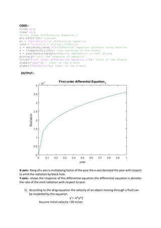
14. 1) Water is being drained from a spout in the bottom of a cylindrical tank. According to
Torricelli’s law the volume V of water left in the tank obeys the differential equation.
y’= -k* sqrt(y)
CODE:-
clc;
close all;
clear all;
f = @(x,y) -x*sqrt(y);% differential equation
y0 = 1; % initial condition
[xa,ya] = ode45(f,[0 1],y0) %diffential equation solver using ode45
plot(xa,ya)% plot the response of equation
title('First order differential Equation_1');% title of the figure
xlabel('time'); % label of the x-axis
ylabel('volume'); %label of the y-axis
OUTPUT:-
X-axis:- The x-axis is the denoted the time in sec with respect the volume of the cylindrical
tank.
Y-axis:- shows the response of the differential equation and it’s denote the volume of a
cylindrical tank.
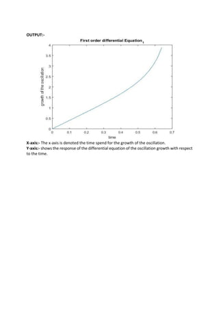
2) Population growth
y’=x*exp(y)
CODE:-
clc;

15. close all;
clear all;
f = @(x,y) x*exp(y);%differential equation
y0 = 1; %initial condition
[xa,ya] = ode45(f,[0 1],y0)%diffential equation solver using ode45
plot(xa,ya)% plot the response
title('First order differential Equation_1');% title of the figure
xlabel('time'); % label of the x-axis
ylabel('population growth'); % label of the y-axis
OUTPUT:-
X-axis:- x-axis is the denoted the time passing for the growth of the population.
Y-axis:- shows the response of the differential equation for the population growth is shown
with respect to time.
3) Temperature change rate with respect to time
y’=0.08(72-y)
CODE:-
clc;
close all;
clear all;
f = @(x,y) 0.08*(72-y);% %differential equation
y0 = 98.6;% initial condition
[xa,ya] = ode45(f,[0 1],y0))%diffential equation solver using ode45
plot(xa,ya)% plot the response of the equation

16. title('First order differential Equation_1');% title of the figure
xlabel('time'); % label of the x-axis
ylabel('Temperature'); % label of the y-axis
OUTPUT:-
X-axis:- x-axis denotes the time for the changing the temperature.
Y-axis:- shows the response of the differential equation of the temperature value with respect
to time.
4) A one company start the selling of the laptop. The laptop they will sold after a x
month. There are 1000 laptop selling possibility.
y’=x(1000-y)
CODE:-
clc;
close all;
clear all;
f = @(x,y) x*(1000-y);% diffential equation
y0 = 0;% initial condition
[xa,ya] = ode45(f,[0 12],y0)% diffential equation solver
plot(xa,ya)% plote the responce of the diffential equation
title('First order differential Equation_1');% title of the figure
xlabel('time in month'); % label to the x axis
ylabel('laptop selling'); % label to the y axis

17. OUTPUT:-
X-axis:- The x-axis is denote the time in terms of month in selling of the laptop.
Y-axis:- shows the response of the differential equation. Also the y axis is given the
information of the selling of the laptop with respect to time.
5) in simple harmonic oscillation obeying the Hooke’s acceleration always being in the
opposite direction of positive leads to an exponential function.
y’=k*exp(y*x)+ k*exp(-(y*x))
CODE:-
clc;
close all;
clear all;
k=2% constant value
f = @(x,y) k*exp(y*x)+ k*exp(-(y*x));% %differential equation
y0 = 0;% initial condition
[xa,ya] = ode45(f,[0 1],y0)%diffential equation solver using ode45
plot(xa,ya)% plot the response of the equation
title('First order differential Equation_1');% title of the figure
xlabel('time'); % label of the x-axis
ylabel('growth of the oscillation'); % label of the y-axis

18. OUTPUT:-
X-axis:- The x-axis is denoted the time spend for the growth of the oscillation.
Y-axis:- shows the response of the differential equation of the oscillation growth with respect
to the time.