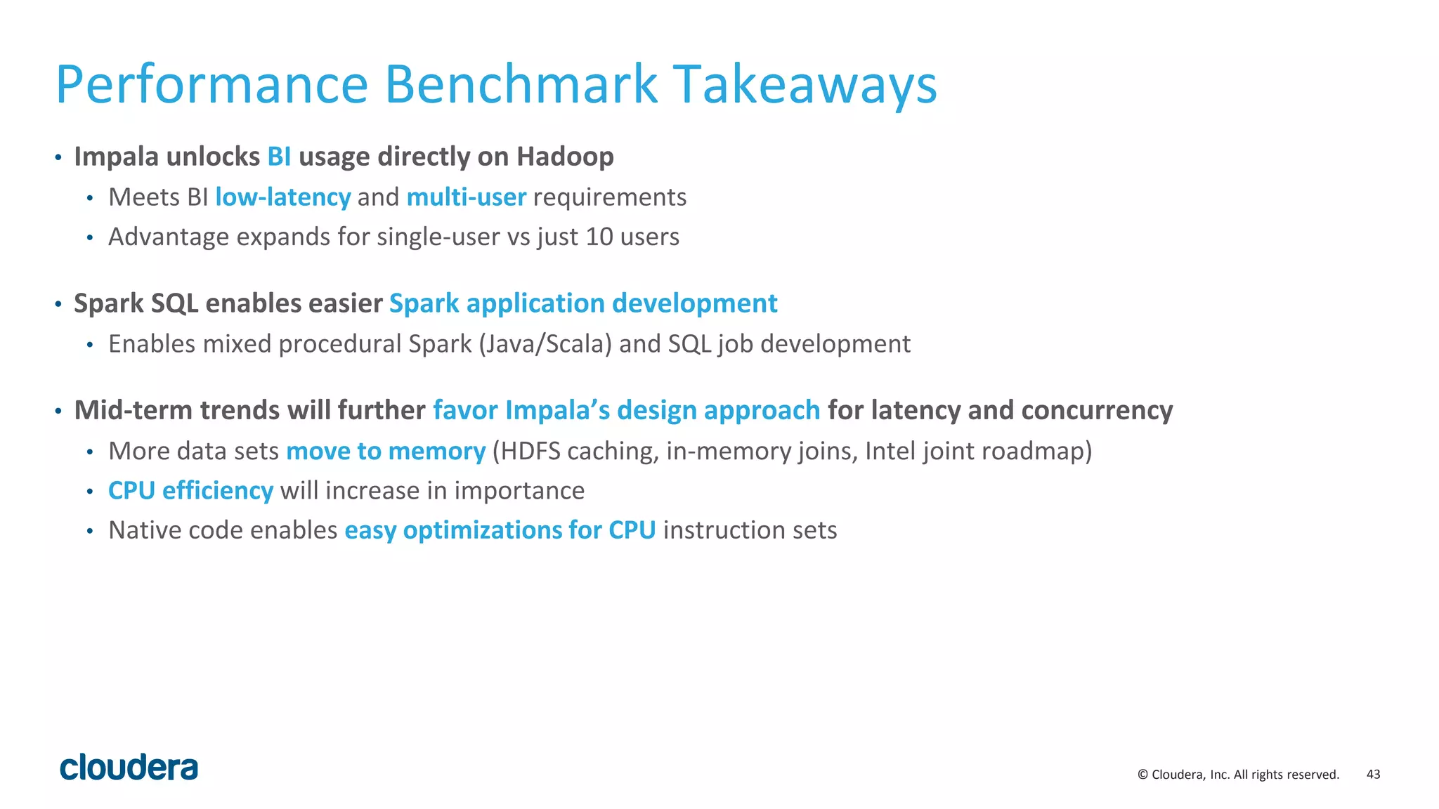
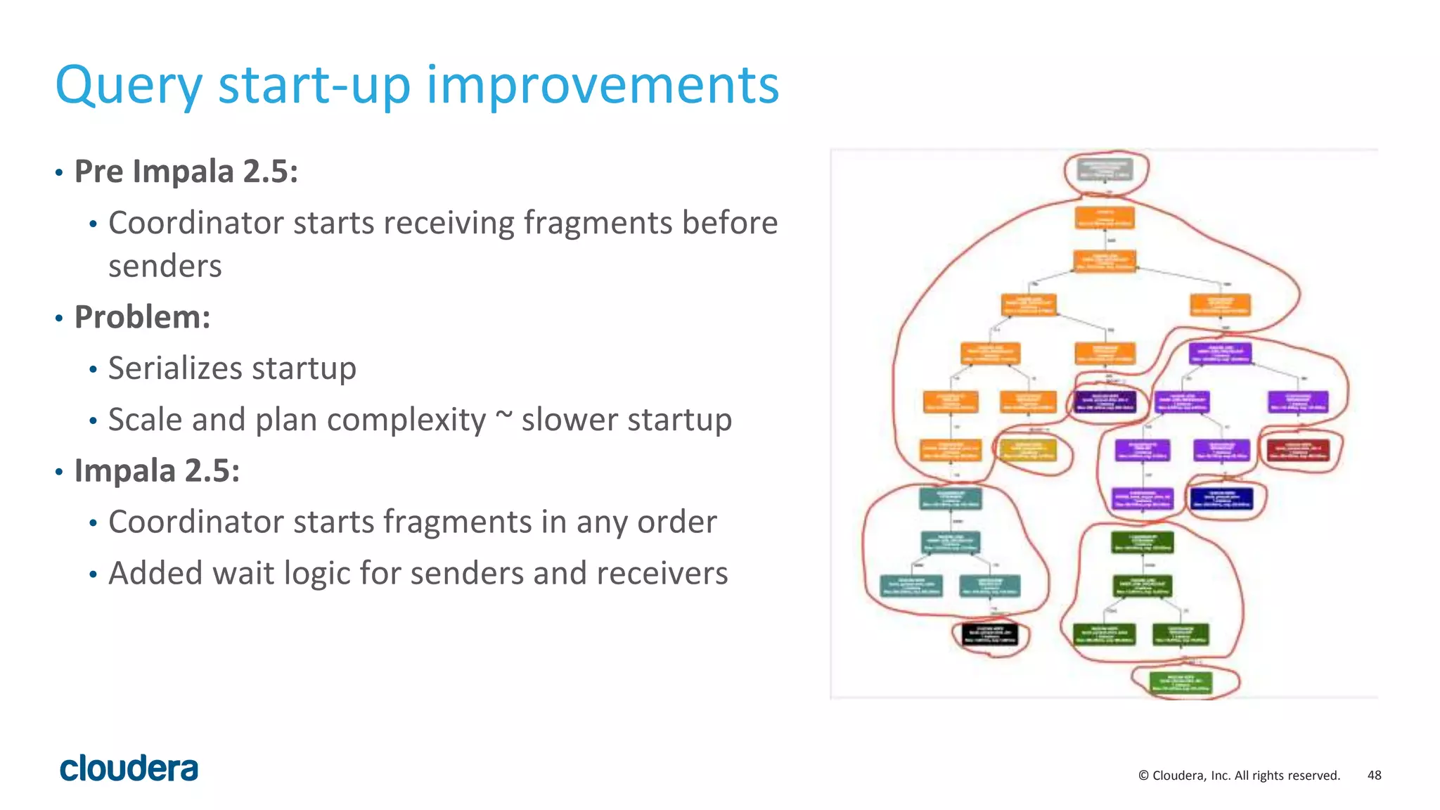
Downloaded 50 times

![25© Cloudera, Inc. All rights reserved.
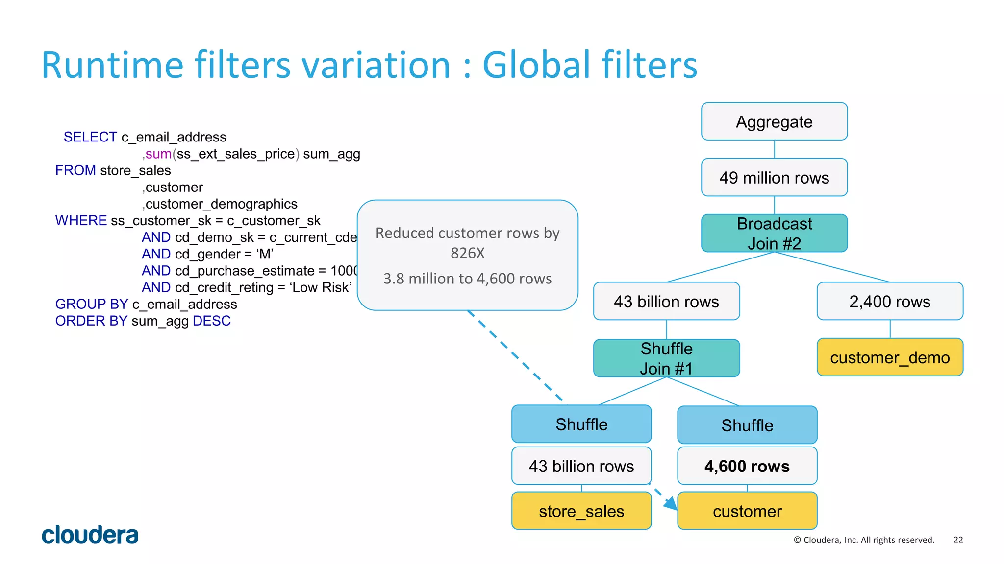
Runtime filters: real-world results
• Runtime filters can be highly effective. Some benchmark queries are more than 30
times faster in Impala 2.5.0.
• As always, depends on your queries, your schemas and your cluster environment.
• By default, runtime filters are enabled in limited ‘local’ mode in Impala 2.5.0. They
can be enabled fully by setting RUNTIME_FILTER_MODE=GLOBAL.
• Other runtime filter parameters include :
• RUNTIME_BLOOM_FILTER_SIZE: [1048576]
• RUNTIME_FILTER_WAIT_TIME_MS: [0]](https://image.slidesharecdn.com/hugmeetupimpala2-160504223558/75/Apache-Impala-incubating-2-5-Performance-Update-25-2048.jpg)
![29© Cloudera, Inc. All rights reserved.
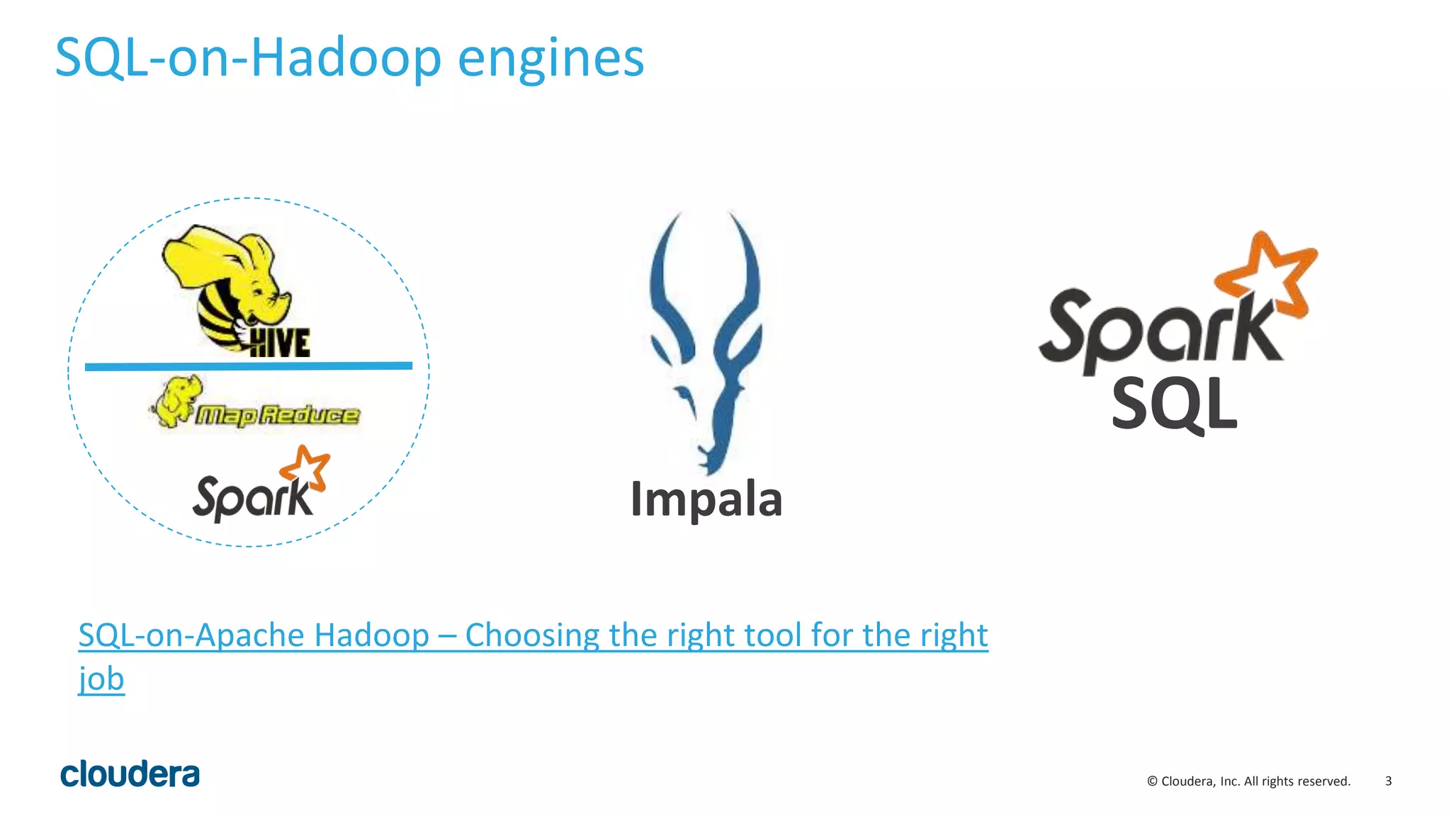
Codegen for Order by & Top-N
void* ExprContext::GetValue(Expr* e, TupleRow* row) {
switch (e->type_.type) {
case TYPE_BOOLEAN: {
..
..
}
case TYPE_TINYINT: {
..
..
}
case TYPE_INT: {
..
.
int Compare(TupleRow* lhs, TupleRow* rhs) const {
for (int i = 0; i < sort_cols_lhs_.size(); ++i) {
void* lhs_value = sort_cols_lhs_[i]->GetValue(lhs);
void* rhs_value = sort_cols_rhs_[i]->GetValue(rhs);
if (lhs_value == NULL && rhs_value != NULL) return nulls_first_[i];
if (lhs_value != NULL && rhs_value == NULL) return -nulls_first_[i];
int result = RawValue::Compare(lhs_value, rhs_value,
sort_cols_lhs_[i]->root()->type());
if (!is_asc_[i]) result = -result;
if (result != 0) return result;
// Otherwise, try the next Expr
}
return 0; // fully equivalent key
}](https://image.slidesharecdn.com/hugmeetupimpala2-160504223558/75/Apache-Impala-incubating-2-5-Performance-Update-29-2048.jpg)
![30© Cloudera, Inc. All rights reserved.
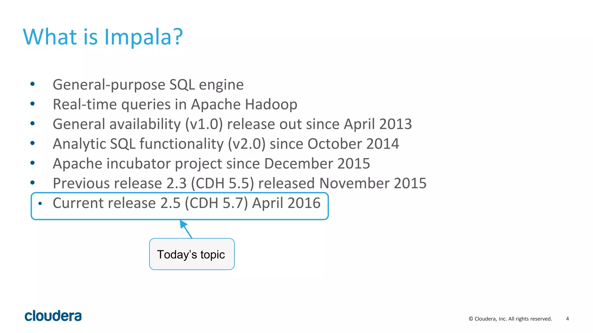
Codegen for Order by & Top-N
int CompareCodgened(TupleRow* lhs, TupleRow* rhs) const {
int64_t lhs_value = sort_columns[i]->GetBigIntVal(lhs); // i = 0
int64_t rhs_value = sort_columns[i]->GetBigIntVal(rhs); // i = 1
int result = lhs_value > rhs_value ? 1 :
(lhs_value < rhs_value ? -1 : 0);
if (result != 0) return result;
// Otherwise, try the next Expr
return 0; // fully equivalent key
}
Codegen code
• Perfectly unrolls “for each grouping column” loop
• No switching on input type(s)
• Removes branching on ASCENDING/DESCENDING,
NULLS FIRST/LAST
Original code
int Compare(TupleRow* lhs, TupleRow* rhs) const {
for (int i = 0; i < sort_cols_lhs_.size(); ++i) {
void* lhs_value = sort_cols_lhs_[i]->GetValue(lhs);
void* rhs_value = sort_cols_rhs_[i]->GetValue(rhs);
if (lhs_value == NULL && rhs_value != NULL) return nulls_first_[i];
if (lhs_value != NULL && rhs_value == NULL) return -nulls_first_[i];
int result = RawValue::Compare(lhs_value, rhs_value,
sort_cols_lhs_[i]->root()->type());
if (!is_asc_[i]) result = -result;
if (result != 0) return result;
// Otherwise, try the next Expr
}
return 0; // fully equivalent key
}](https://image.slidesharecdn.com/hugmeetupimpala2-160504223558/75/Apache-Impala-incubating-2-5-Performance-Update-30-2048.jpg)
![31© Cloudera, Inc. All rights reserved.
Codegen for Order by & Top-N
int CompareCodgened(TupleRow* lhs, TupleRow* rhs) const {
int64_t lhs_value = sort_columns[i]->GetBigIntVal(lhs); // i = 0
int64_t rhs_value = sort_columns[i]->GetBigIntVal(rhs); // i = 1
int result = lhs_value > rhs_value ? 1 :
(lhs_value < rhs_value ? -1 : 0);
if (result != 0) return result;
// Otherwise, try the next Expr
return 0; // fully equivalent key
}
Codegen code
• Perfectly unrolls “for each grouping column” loop
• No switching on input type(s)
• Removes branching on ASCENDING/DESCENDING,
NULLS FIRST/LAST
Original code
int Compare(TupleRow* lhs, TupleRow* rhs) const {
for (int i = 0; i < sort_cols_lhs_.size(); ++i) {
void* lhs_value = sort_cols_lhs_[i]->GetValue(lhs);
void* rhs_value = sort_cols_rhs_[i]->GetValue(rhs);
if (lhs_value == NULL && rhs_value != NULL) return nulls_first_[i];
if (lhs_value != NULL && rhs_value == NULL) return -nulls_first_[i];
int result = RawValue::Compare(lhs_value, rhs_value,
sort_cols_lhs_[i]->root()->type());
if (!is_asc_[i]) result = -result;
if (result != 0) return result;
// Otherwise, try the next Expr
}
return 0; // fully equivalent key
}
10x more efficient
code](https://image.slidesharecdn.com/hugmeetupimpala2-160504223558/75/Apache-Impala-incubating-2-5-Performance-Update-31-2048.jpg)
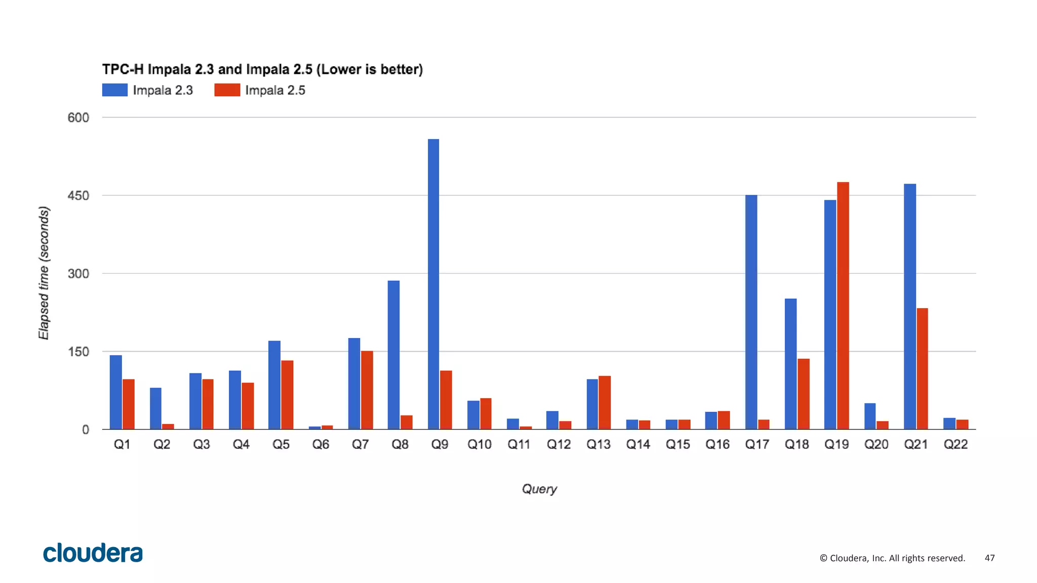
![38© Cloudera, Inc. All rights reserved.
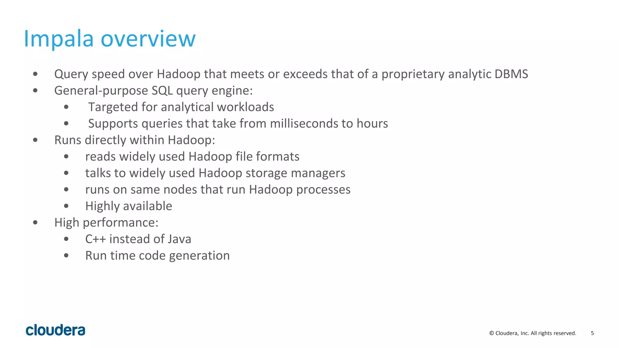
Optimization for partition keys scan
• Use metadata to avoid table accesses for partition key scans:
• select min(month), max(year) from functional.alltypes;
• month, year are partition keys of the table
• Enabled by query option OPTIMIZE_PARTITION_KEY_SCANS
• Applicable:
• min(), max(), ndv() and aggregate functions with distinct keyword
• partition keys only
01:AGGREGATE [FINALIZE]
| output: min(month),max(year)
|
00:UNION
constant-operands=24
03:AGGREGATE [FINALIZE]
| output: min:merge(month), max:merge(year)
|
02:EXCHANGE [UNPARTITIONED]
|
01:AGGREGATE
| output: min(month), max(year)
|
00:SCAN HDFS [functional.alltypes]
partitions=24/24 files=24 size=478.45KB
Plan without optimization Plan with optimization](https://image.slidesharecdn.com/hugmeetupimpala2-160504223558/75/Apache-Impala-incubating-2-5-Performance-Update-38-2048.jpg)


The document discusses performance improvements in Apache Impala 2.5, including runtime filters, improved cardinality estimation and join ordering, faster query startup times, and expanded use of LLVM code generation. Runtime filters allow filtering of unnecessary rows during query execution based on predicates, improving performance significantly for some queries. Cardinality estimation and join ordering were enhanced to produce more accurate estimates. Code generation was extended to support additional data types and operators like order by and top-n. Benchmark results showed speedups of over 30x for some queries in Impala 2.5 compared to earlier versions.