The document provides information about contact details for Hemant Trivedi and then discusses analysis of variance (ANOVA) techniques, including one-way, two-way, and three or more way ANOVA. It provides an example of using ANOVA to determine the best type of packaging among three options. The document also includes information about chi square tests, including their applications and a formula. It provides two examples for chi square test exercises. Finally, it discusses fundamentals of variables, types of tests, hypotheses, and choosing a significance level.

1. Contact
Hemant Trivedi
59-A, A-Road, Bhupalpura, Udaipur (Rajasthan)
E-mail: trivedihemant@yahoo.com
Mobile: 9414162917

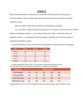
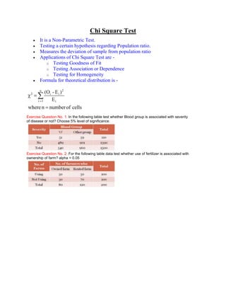
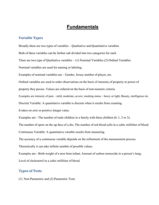
2. ANOVA
When measurement data are influenced by several kind of effects operating simultaneously or
when more than two means of independent samples are involved, analysis of variance technique
(ANOVA) is used.
One way ANOVA (One criteria on the basis of which data is classified).
Two way ANOVA (Data is classified on the basis of two criteria) or Three or more way ANOVA.
Estimate of population variance i. e. mean square between the sample is calculated, estimate of
population variance i. e. mean square within the sample is calculated, ratio of the two variance is
calculated and inference is drawn.
— Example: Manufacturer wants to know which type of packaging is best among three types of packaging.
— study compared the effects of four 1-month point-of-purchase promotions on sales.
A
The unit sales for five stores using all four promotions in different months follow.
Calculate the F-ratio. At 0.01 level of significance do the promotions produce different effects on sales

3. Chi Square Test
It is a Non-Parametric Test.
Testing a certain hypothesis regarding Population ratio.
Measures the deviation of sample from population ratio
Applications of Chi Square Test are -
o Testing Goodness of Fit
o Testing Association or Dependence
o Testing for Homogeneity
Formula for theoretical distribution is -
Exercise Question No. 1: In the following table test whether Blood group is associated with severity
of disease or not? Choose 5% level of significance.
Exercise Question No. 2: For the following table data test whether use of fertilizer is associated with
ownership of farm? alpha = 0.05

4. Fundamentals
Variable Types
Broadly there are two types of variables – Qualitative and Quantitative variables
Both of these variables can be further sub divided into two categories for each
There are two type of Qualitative variables – (1) Nominal Variables (2) Ordinal Variables
Nominal variables are used for naming or labeling.
Examples of nominal variables are – Gender, Jersey number of player, etc.
Ordinal variables are used to order observations on the basis of intensity of property or power of
property they posses. Values are ordered on the basis of non-numeric criteria.
Examples are intensity of pain – mild, moderate, severe; smoking status – heavy or light; Beauty, intelligence etc.
Discrete Variable: A quantitative variable is discrete when it results from counting.
It takes on zero or positive integer value.
Examples are - The number of male children in a family with three children (0, 1, 2 or 3),
The number of spots on the up-face of a die; The number of red blood cells in a cubic milliliter of blood
Continuous Variable: A quantitative variable results from measuring.
The accuracy of a continuous variable depends on the refinement of the measurement process.
Theoretically it can take infinite number of possible values.
Examples are - Birth weight of a new born infant; Amount of carbon monoxide in a person’s lung;
Level of cholesterol in a cubic milliliter of blood.
Types of Tests
(1) Non-Parametric and (2) Parametric Tests

5. Non-Parametric tests - Assumes that variables are measured on nominal or ordinal scale.
These tests do not make any assumption about the shape of the population from which the samples are
drawn hence also known as “distribution free tests” or more commonly “Non-parametric tests”.
Examples : Sign test, Chi square test, Kruskal – Wallis test, Rank correlation, etc.
Parametric Tests - One that is based on certain parameters. Our samples were either large or comes
form normally distributed population. Examples are - Student’s t-test, F-test, Z-test , etc.
Hypothesis
There are two types of statistical hypothesis – (1) Null hypothesis (2) Alternate hypothesis
Null Hypothesis is hypothesis of no difference and is generally represented by H0 and alternative
hypothesis is just opposite of null hypothesis and is represented by Ha.
e.g. H0 = Sample mean = Population mean
Choosing level of Significance
A statistical hypothesis test provides a process for accepting or rejecting null hypothesis (H0) OR
rejecting or accepting alternative hypothesis (H1), while knowing the error rate associated with decision.
The null hypothesis (H0) is either true or false and there are two possible decision accept or reject null
hypothesis (H0) creating four possible outcomes to a statistical hypothesis test.
Decision H0 is true H0 is false
Accept H0 Correct Decision Type II error ( )
Reject H0 Type I error ( ) Correct Decision
A type I error occurs when a true null hypothesis is rejected or when a false alternative hypothesis is

6. accepted i.e. a random variation has been mistaken for a “real” difference
Type I error is called level of significance and it is decided prior to experiment.
A significance level of say 1% implies that the researcher is running the risk of being wrong in accepting
or rejecting the hypothesis in 1 out of every 100 occasions.
It is possible to test a hypothesis at any level of significance.
A type II error occurs when a null hypothesis is accepted when alternative hypothesis is true.
(1 – is known as power of test
Test for Difference of Means
To test whether there is significant difference between means of two samples or between sample
and population mean test for difference of means is applied. Here also there are four situations viz.
1. When sample is large and to test difference between means of sample and population
2. When sample is large and to test difference between means of two independent samples
3. When sample is small and to test difference between means of sample and population
4. When sample is small and to test difference between means of two independent samples.
5. Paired t - test
The formulas for these test are taught to you in the class. Given below are the problems related to
these situations. Solve them.
When sample is large and to test difference between means of sample and population
Exercise Question No. 3
In a survey on hearing levels of school children with normal hearing it was found
that in the frequency 500 cycles per second, 62 children tested in the sound proof
room has a mean hearing threshold of 15.5 decibels with a standard deviation of
6.5. 76 comparable children who were tested in the field had a mean threshold of
20.0 decibels with a standard deviation of 7.1. Test if there is any difference between
the hearing levels recorded in the sound proof room in the field.
When sample is large and to test difference between means of two independent samples
Exercise Question No. 4
A potential buyer want to purchase bulbs in bulk and he wants to decide bulb of which
company A or B he should purchase?

7. Which of the two brands is of better quality?
When sample is small and to test difference between means of sample and population
Exercise Question No. 5
A health survey in a few village revealed that the normal serum protein value of children in that
locality is 7.0 g/100 ml. A group of 16 children who received high protein food for a period of 6
months had serum protein value is given in the table. Can we consider that the mean serum
protein level of those who were fed on high protein diet is different from that of the general
population?
When sample is small and to test difference between means of two
independent samples
Exercise Question No. 6
— a feeding trial 17 children were given high protein food supplement to their normal
In
diet and 15 comparable children were kept under normal diet. They were kept on this
feeding for 7 months. At the end of this study the change in the (initial – final) Hb level
of two groups was assessed (data given in table). Does it provides any evidence to say that the
change in the Hb level of the children who received high protein food is different from the
control group?

8. Paired Sample t-test
Exercise Question No. 7
Twelve pre-school children were given a supplement of multi-purpose food for a
period of four months. Their skin fold thickness (in mm) was measured before the
commencement of the programme and also at the end. Test if there is any change in
skin fold thickness.

9. Time Series Analysis
The term “Time Series” is used to refer to any group of statistical information accumulated over
regular interval.
A time series is an arrangement of statistical data in a chronological order in occurrence with its
time of
occurrence.
Examples are
— series relating to prices,
— production and consumption of various commodities,
— agriculture and industrial production,
— national income and foreign exchange reserves,
— investments, sales and profits of business houses,
— bank deposits and clearings,
— prices and dividends of shares in a stock exchange markets
Time series analysis is used to detect pattern of change in statistical information over regular
interval of time.
We project these patterns to arrive at an estimate for the future
There are four kinds of variation or change involved in time-series analysis
— Secular trend
— Cyclical fluctuation
— Seasonal variation
— Irregular or random variations
Secular trend
— The value of variable tends to increase or decrease over a long period of time.
— E.g. The steady increase in the cost of living recorded by Consumer Price Index.

10. — For an individual year cost of living varies a great deal but if we examine a long
term period we see that the trend is towards steady increase.
Cyclical fluctuation
— Business cycle.
— Business cycle hits a peak above the trend line.
— Business activity hitting a low point below the trend line.
— The time between hitting peaks and falling to low points is at least 1 year and it can
be as many as 15-20 years.
— Cyclical movements do not follow any regular pattern but move in somewhat
unpredictable manner.
Seasonal variation
— Seasonal variation involves pattern of change within a year that tend to be repeated
from year to year.
— E.g. a physician can expect a substantial increase in the number of flu cases every
winter.
Sale of ice cream
— Sale of crackers in festive season.
— Because of regular pattern, they are useful in forecasting the future.
Irregular variations
— In many situations the value of a variable is completely unpredictable, changing in a
random manner. Irregular variation describes such movements.
— Results of some unexpected events.
In most of the instances a time series will contain several of these components.
Thus, overall variation in a single time series can be described in terms of these four
different kinds of variations.
Trend Analysis
Of the four components of time series secular trend represents the long term direction
of the series.
— To describe the trend component we can fit a trend line by the method of least
squares.
— Reasons for studying secular trends
— Historical patterns
— Projecting past patterns or trends into future

11. — Eliminate the trend component
— Trends can be linear or curvilinear.
— Fitting the linear trend
Equation for estimating a straight line
Y = a + bX where a = intercept; b = slope of line; Y = dependent variable and X = Time
Equation for estimating a and b when time is coded
Equation for a
Example