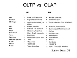
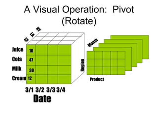
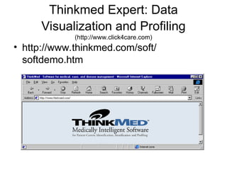
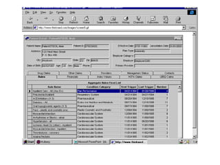
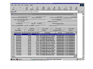
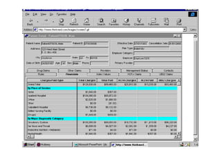
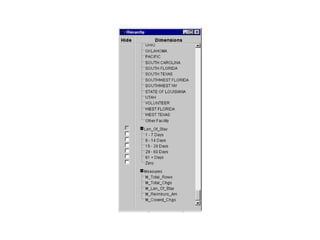
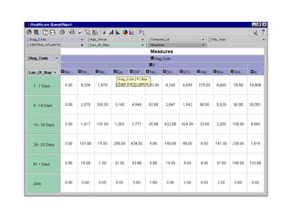
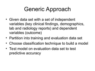
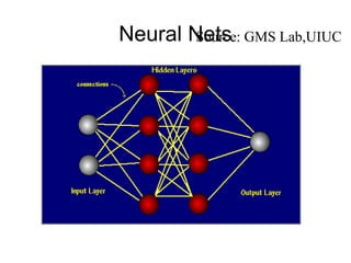
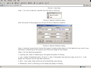
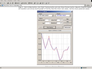
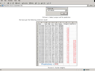
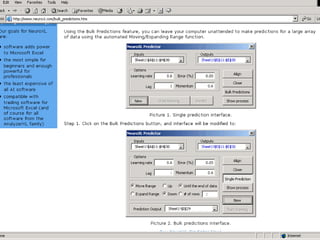
The document outlines the fundamentals of Online Analytical Processing (OLAP) and compares it to Online Transaction Processing (OLTP), highlighting OLAP's ability to support ad-hoc querying and provide multidimensional views of data for business analysts. It discusses various OLAP server types, including MOLAP, ROLAP, and HOLAP, and their respective advantages and disadvantages, as well as tools for data extraction, transformation, load (ETL), and reporting. Additionally, it covers data mining methods and approaches to knowledge discovery in databases, alongside the importance of data visualization in analyzing complex relationships.

1. OLAP fundamentals

2. OLAP Conceptual Data Model
 Goal of OLAP is to support ad-hoc querying for the
business analyst
 Business analysts are familiar with spreadsheets
 Extend spreadsheet analysis model to work with
warehouse data
 Multidimensional view of data is the foundation of
OLAP

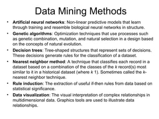
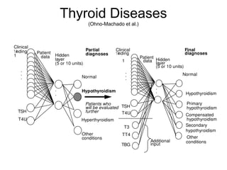
3. OLTP vs. OLAP
 On-Line Transaction Processing (OLTP):
– technology used to perform updates on operational
or transactional systems (e.g., point of sale systems)
 On-Line Analytical Processing (OLAP):
– technology used to perform complex analysis of the
data in a data warehouse
OLAP is a category of software technology that enables analysts,
managers, and executives to gain insight into data through fast,
consistent, interactive access to a wide variety of possible views
of information that has been transformed from raw data to reflect
the dimensionality of the enterprise as understood by the user.
[source: OLAP Council: www.olapcouncil.org]

4. OLTP vs. OLAP
• Clerk, IT Professional
• Day to day operations
• Application-oriented (E-R
based)
• Current, Isolated
• Detailed, Flat relational
• Structured, Repetitive
• Short, Simple transaction
• Read/write
• Index/hash on prim. Key
• Tens
• Thousands
• 100 MB-GB
• Trans. throughput
• Knowledge worker
• Decision support
• Subject-oriented (Star, snowflake)
• Historical, Consolidated
• Summarized, Multidimensional
• Ad hoc
• Complex query
• Read Mostly
• Lots of Scans
• Millions
• Hundreds
• 100GB-TB
• Query throughput, response
User
Function
DB Design
Data
View
Usage
Unit of work
Access
Operations
# Records accessed
#Users
Db size
Metric
OLTP
OLTP OLAP
OLAP
Source: Datta, GT

5. Approaches to OLAP Servers
• Multidimensional OLAP (MOLAP)
– Array-based storage structures
– Direct access to array data structures
– Example: Essbase (Arbor)
• Relational OLAP (ROLAP)
– Relational and Specialized Relational DBMS to store and
manage warehouse data
– OLAP middleware to support missing pieces
• Optimize for each DBMS backend
• Aggregation Navigation Logic
• Additional tools and services
– Example: Microstrategy, MetaCube (Informix)

6. MOLAP

7. Multidimensional Data
10
10
47
47
30
30
12
12
Juice
Juice
Cola
Cola
Milk
Milk
Cream
Cream
N
Y
N
Y
L
A
L
A
S
F
S
F
Sales
Sales
Volume
Volume
as a
as a
function
function
of time,
of time,
city and
city and
product
product
3/1 3/2 3/3 3/4
3/1 3/2 3/3 3/4
Date
Date

8. Operations in Multidimensional Data
Model
• Aggregation (roll-up)
– dimension reduction: e.g., total sales by city
– summarization over aggregate hierarchy: e.g., total sales by city
and year -> total sales by region and by year
• Selection (slice) defines a subcube
– e.g., sales where city = Palo Alto and date = 1/15/96
• Navigation to detailed data (drill-down)
– e.g., (sales - expense) by city, top 3% of cities by average
income
• Visualization Operations (e.g., Pivot)

9. A Visual Operation: Pivot
(Rotate)
10
10
47
47
30
30
12
12
Juice
Juice
Cola
Cola
Milk
Milk
Cream
Cream
N
Y
N
Y
L
A
L
A
S
F
S
F
3/1 3/2 3/3 3/4
3/1 3/2 3/3 3/4
Date
Date
Month
Month
Region
Region
Product
Product

10. Thinkmed Expert: Data
Visualization and Profiling
(http://www.click4care.com)
• http://www.thinkmed.com/soft/
softdemo.htm

11. ThinkMed Expert
• Processing of consolidated patient
demographic, administrative and claims
information using knowledge-based rules
• Goal is to identify patients at risk in order
to intervene and affect financial and
clinical outcomes

12. Vignette
• High risk diabetes program
• Need to identify
– patients that have severe disease
– patients that require individual attention and
assessment by case managers
• Status quo
– rely on provider referrals
– rely on dollar cutoffs to identify expensive
patients

13. Vignette
• ThinkMed approach
– Interactive query facility with filters to identify
patients in the database that have desired
attributes
• patients that are diabetic and that have cardiac,
renal, vascular or neurological conditions (use of
codes or natural language boolean queries)
• visualize financial data by charge type

20. Administrative DSS using
WOLAP

27. ROLAP

28. Relational DBMS as Warehouse
Server
• Schema design
• Specialized scan, indexing and join
techniques
• Handling of aggregate views (querying and
materialization)
• Supporting query language extensions
beyond SQL
• Complex query processing and optimization
• Data partitioning and parallelism

29. MOLAP vs. OLAP
• Commercial offerings of both types are
available
• In general, MOLAP is good for smaller
warehouses and is optimized for canned
queries
• In general, ROLAP is more flexible and
leverages relational technology on the data
server and uses a ROLAP server as
intermediary. May pay a performance penalty
to realize flexibility

30. Tools: Warehouse Servers
 The RDBMS dominates:
 Oracle 8i/9i
 IBM DB2
 Microsoft SQL Server
 Informix (IBM)
 Red Brick Warehouse (Informix/IBM)
 NCR Teradata
 Sybase…

31. Tools: OLAP Servers
 Support multidimensional OLAP queries
 Often characterized by how the underlying data stored
 Relational OLAP (ROLAP) Servers
 Data stored in relational tables
 Examples: Microstrategy Intelligence Server, MetaCube
(Informix/IBM)
 Multidimensional OLAP (MOLAP) Servers
 Data stored in array-based structures
 Examples: Hyperion Essbase, Fusion (Information Builders)
 Hybrid OLAP (HOLAP)
 Examples: PowerPlay (Cognos), Brio, Microsoft Analysis
Services, Oracle Advanced Analytic Services

32. Tools: Extraction,
Transformation, & Load (ETL)
 Cognos Accelerator
 Copy Manager, Data Migrator for SAP,
PeopleSoft (Information Builders)
 DataPropagator (IBM)
 ETI Extract (Evolutionary Technologies)
 Sagent Solution (Sagent Technology)
 PowerMart (Informatica)…

33. Tools: Report & Query
 Actuate e.Reporting Suite (Actuate)
 Brio One (Brio Technologies)
 Business Objects
 Crystal Reports (Crystal Decisions)
 Impromptu (Cognos)
 Oracle Discoverer, Oracle Reports
 QMF (IBM)
 SAS Enterprise Reporter…

34. Tools: Data Mining
 BusinessMiner (Business Objects)
 Decision Series (Accrue)
 Enterprise Miner (SAS)
 Intelligent Miner (IBM)
 Oracle Data Mining Suite
 Scenario (Cognos)…

35. Data Mining: A brief overview
Discovering patterns in data

36. Intelligent Problem Solving
• Knowledge = Facts + Beliefs + Heuristics
• Success = Finding a good-enough answer
with the resources available
• Search efficiency directly affects success

37. Focus on Knowledge
• Several difficult problems do not have
tractable algorithmic solutions
• Human experts achieve high level of
performance through the application of
quality knowledge
• Knowledge in itself is a resource.
Extracting it from humans and putting it
in computable forms reduces the cost of
knowledge reproduction and exploitation

38. Value of Information
• Exponential growth in information storage
• Tremendous increase in information
retrieval
• Information is a factor of production
• Knowledge is lost due to information
overload

39. KDD vs. DM
• Knowledge discovery in databases
– “non-trivial extraction of implicit, previously
unknown and potentially useful knowledge
from data”
• Data mining
– Discovery stage of KDD

40. Knowledge discovery in databases
• Problem definition
• Data selection
• Cleaning
• Enrichment
• Coding and organization
• DATA MINING
• Reporting

41. Problem Definition
• Examples
– What factors affect treatment compliance?
– Are there demographic differences in drug
effectiveness?
– Does patient retention differ among doctors
and diagnoses?

42. Data Selection
• Which patients?
• Which doctors?
• Which diagnoses?
• Which treatments?
• Which visits?
• Which outcomes?

43. Cleaning
• Removal of duplicate records
• Removal of records with gaps
• Enforcement of check constraints
• Removal of null values
• Removal of implausible frequent values

44. Enrichment
• Supplementing operational data with
outside data sources
– Pharmacological research results
– Demographic norms
– Epidemiological findings
– Cost factors
– Medium range predictions

45. Coding and Organizing
• Un-Normalizing
• Rescaling
• Nonlinear transformations
• Categorizing
• Recoding, especially of null values

46. Reporting
• Key findings
• Precision
• Visualization
• Sensitivity analysis

47. Why Data Mining?
 Claims analysis - determine which medical procedures
are claimed together.
 Predict which customers will buy new policies.
 Identify behavior patterns of risky customers.
 Identify fraudulent behavior.
 Characterize patient behavior to predict office visits.
 Identify successful medical therapies for different
illnesses.

48. Data Mining Methods
• Verification
– OLAP flavors
– Browsing of data or querying of data
– Human assisted exploration of data
• Discovery
– Using algorithms to discover rules or patterns

49. Data Mining Methods
• Artificial neural networks: Non-linear predictive models that learn
through training and resemble biological neural networks in structure.
• Genetic algorithms: Optimization techniques that use processes such
as genetic combination, mutation, and natural selection in a design based
on the concepts of natural evolution.
• Decision trees: Tree-shaped structures that represent sets of decisions.
These decisions generate rules for the classification of a dataset.
• Nearest neighbor method: A technique that classifies each record in a
dataset based on a combination of the classes of the k record(s) most
similar to it in a historical dataset (where k 1). Sometimes called the k-
nearest neighbor technique.
• Rule induction: The extraction of useful if-then rules from data based on
statistical significance.
• Data visualization: The visual interpretation of complex relationships in
multidimensional data. Graphics tools are used to illustrate data
relationships.

50. Types of discovery
• Association
– identifying items in a collection that occur together
• popular in marketing
• Sequential patterns
– associations over time
• Classification
– predictive modeling to determine if an item
belongs to a known group
• treatment at home vs. at the hospital
• Clustering
– discovering groups or categories

51. Association: A simple example
• Total transactions in a hardware store = 1000
• number which include hammer = 50
• number which include nails = 80
• number which include lumber = 20
• number which include hammer and nails = 15
• number which include nails and lumber = 10
• number which include hammer, nails and
lumber = 5

52. Association Example
• Support for hammer and nails = .015
(15/1000)
• Support for hammer, nails and lumber = .005
(5/1000)
• Confidence of “hammer ==>nails” =.3 (15/50)
• Confidence of “nails ==> hammer”=15/80
• Confidence of “hammer and nails ===>
lumber” = 5/15
• Confidence of “lumber ==> hammer and
nails” = 5/20

53. Association: Summary
• Description of relationships observed in
data
• Simple use of bayes theorem to identify
conditional probabilities
• Useful if data is representative to take
action
– market basket analysis

54. Bayesian Analysis
Bayesian
Analysis
New Information
Prior Probabilities
Posterior
Probabilities

55. A Medical Test
A doctor must treat a patient who has a tumor. He
knows that 70 percent of similar tumors are benign. He
can perform a test, but the test is not perfectly
accurate. If the tumor is malignant, long experience
with the test indicates that the probability is 80 percent
that the test will be positive, and 10 percent that it will
be negative; 10 percent of the tests are inconclusive. If
the tumor is benign, the probability is 70 percent that
the test will be negative, 20 percent that it will be
positive; again, 10 percent of the tests are
inconclusive. What is the significance of a positive or
negative test?

56. .7 Benign
.3 Malignant
.2 Test positive
.1 Inconclusive
.7 Test negative
.8 Test positive
.1 Inconclusive
.1 Test negative

57. Test Positive
Test inconclusive
Test negative
Benign
Malignant
Benign
Malignant
Benign
Malignant

58. .7 Benign
.3 Malignant
.2 Test Positive
.1 Test inconclusive
.7 Test negative
.8 Test positive
.1 Test inconclusive
.1 Test negative
Benign
.14/.38 = .368
Malignant
.27/.38 = .632
Path probability
.14
.07
.49
.24
.03
.03
Path probability
.14
.24
.07
.03
.49
.03
Benign
.07/.10 = .7
Malignant
.03/.10 = .3
Benign
.49/.52 = .942
Malignant
.03/.52 = .058
Test positive
.14 + .24 = .38
Test inconclusive
.07 + .03 = .10
Test negative
.49 + .03 = .52

59. Decision pro

60. Rule-based Systems
A rule-based system consists of a data
base containing the valid facts, the rules
for inferring new facts and the rule
interpreter for controlling the inference
process
• Goal-directed
• Data-directed
• Hypothesis-directed

61. Classification
• Identify the characteristics that indicate the
group to which each case belongs
– pneumonia patients: treat at home vs. treat in
the hospital
– several methods available for classification
• regression
• neural networks
• decision trees

62. Generic Approach
• Given data set with a set of independent
variables (key clinical findings, demographics,
lab and radiology reports) and dependent
variables (outcome)
• Partition into training and evaluation data set
• Choose classification technique to build a model
• Test model on evaluation data set to test
predictive accuracy

63. Multiple Regression
• Statistical Approach
– independent variables: problem
characteristics
– dependent variables: decision
• the general form of the relationship has to be
known in advance (e.g., linear, quadratic, etc.)

64. Neural Nets
Source: GMS Lab,UIUC

65. Neural Nets
Source: GMS Lab,UIUC

66. Neural networks
• Nodes are variables
• Weights on links by training the network
on the data
• Model designer has to make choices
about the structure of the network and
the technique used to determine the
weights
• Once trained on the data, the neural
network can be used for prediction

67. Neural Networks: Summary
• widely used classification technique
• mostly used as a black box for
predictions after training
• difficult to interpret the weights on the
links in the network
• can be used with both numeric and
categorical data

68. Myocardial Infarction Network
(Ohno-Machado et al.)
0.8
Myocardial Infarction
“Probability” of MI
1
1
2 1
50
Male
Age
Smoker
ECG: ST
Pain
Intensity
4
Pain
Duration Elevation

69. Thyroid Diseases
(Ohno-Machado et al.)
Hidden
layer
Patient
data
Partial
diagnoses
TSH
T4U
Clinical
¼
nding
1
.
.
.
.
.
(5 or 10 units)
Normal
Hyperthyroidism
Hypothyroidism
Other
conditions
Patients who
will be evaluated
further
Hidden
layer
Patient
data
Final
diagnoses
TSH
T4U
Clinical
¼
nding
1
.
.
.
T3
TT4
TBG
.
.
(5 or 10 units)
Normal
Primary
hypothyroidism
Compensated
hypothyroidism
Secondary
hypothyroidism
Hypothyroidism
Other
conditions
Additional
input

81. Model Comparison
(Ohno-Machado et al.)
Modeling Examples Explanation
Effort Needed Provided
Rule-based Exp. Syst. high low high
Bayesian Nets high low moderate
Classification Trees low high “high”
Neural Nets low high low
Regression Models high moderate moderate

82. Summary
Neural Networks are
• mathematical models that resemble nonlinear regression
models, but are also useful to model nonlinearly
separable spaces
• “knowledge acquisition tools” that learn from examples
• Neural Networks in Medicine are used for:
– pattern recognition (images, diseases, etc.)
– exploratory analysis, control
– predictive models

83. Case for Change(PriceWaterhouseCoopers 2003)
• Creating the future hospital system
– Focus on high-margin, high-volume, high-
quality services
– Strategically price services
– Understand demands on workers
– Renew and replace aging physical structures
– Provide information at the fingertips
– Support physicians through new technologies

84. Case for Change(PriceWaterhouseCoopers 2003)
• Creating the future payor system
– Pay for performance
– Implement self-service tools to lower costs
and shift responsibility
– Target high-volume users through
predictive modeling
– Move to single-platform IT and data
warehousing systems
– Weigh opportunities, dilemmas amid public
and private gaps