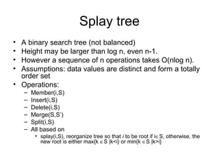
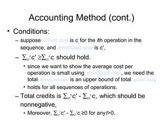
Amortized analysis allows analyzing the average performance of a sequence of operations on a data structure, even if some operations are expensive. There are three main methods for amortized analysis: aggregate analysis, accounting method, and potential method. The accounting method assigns differing amortized costs to operations. When the amortized cost is higher than actual cost, the difference is stored as credit. Later operations may use accumulated credits when their amortized cost is lower than actual cost. The potential method associates potential energy with the data structure as a whole. The amortized cost of an operation is the actual cost plus the change in potential. If potential never decreases, the total amortized cost bounds the total

1. Amortized Analysis (chap. 17)
• Not just consider one operation, but a sequence of
operations on a given data structure.
• Average cost over a sequence of operations.
• Probabilistic analysis:
– Average case running time: average over all possible inputs for
one algorithm (operation).
– If using probability, called expected running time.
• Amortized analysis:
– No involvement of probability
– Average performance on a sequence of operations, even some
operation is expensive.
– Guarantee average performance of each operation among the
sequence in worst case.

2. Three Methods of Amortized Analysis
• Aggregate analysis:
– Total cost of n operations/n,
• Accounting method:
– Assign each type of operation an (different) amortized cost
– overcharge some operations,
– store the overcharge as credit on specific objects,
– then use the credit for compensation for some later
operations.
• Potential method:
– Same as accounting method
– But store the credit as “potential energy” and as a whole.

3. Example for amortized analysis
• Stack operations:
– PUSH(S,x), O(1)
– POP(S), O(1)
– MULTIPOP(S,k), min(s,k)
• while not STACK-EMPTY(S) and k>0
• do POP(S)
• k=k-1
• Let us consider a sequence of n PUSH, POP,
MULTIPOP.
– The worst case cost for MULTIPOP in the sequence is
O(n), since the stack size is at most n.
– thus the cost of the sequence is O(n2
). Correct, but not
tight.

4. Aggregate Analysis
• In fact, a sequence of n operations on an
initially empty stack cost at most O(n). Why?
Each object can be POP only once (including in MULTIPOP) for each time
it is PUSHed. #POPs is at most #PUSHs, which is at most n.
Thus the average cost of an operation is O(n)/n = O(1).
Amortized cost in aggregate analysis is defined to be average cost.

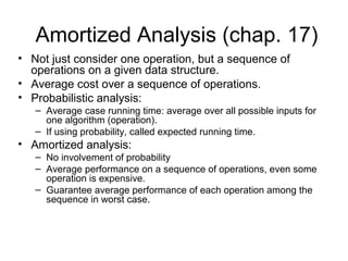
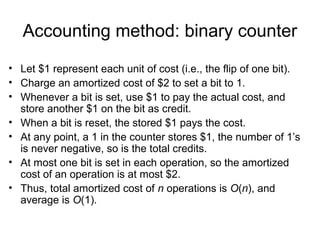
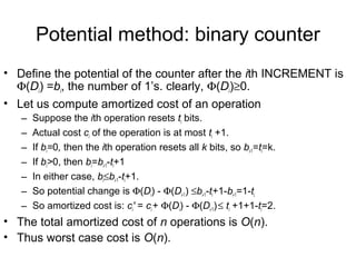
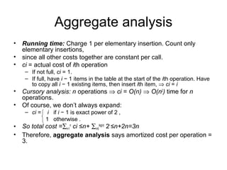
5. Another example: increasing a binary counter
• Binary counter of length k, A[0..k-1] of bit
array.
• INCREMENT(A)
1. i0
2. while i<k and A[i]=1
3. do A[i]0 (flip, reset)
4. ii+1
5. if i<k
6. then A[i]1 (flip, set)

6. Analysis of INCREMENT(A)
• Cursory analysis:
– A single execution of INCREMENT takes
O(k) in the worst case (when A contains all
1s)
– So a sequence of n executions takes O(nk)
in worst case (suppose initial counter is 0).
– This bound is correct, but not tight.
• The tight bound is O(n) for n
executions.

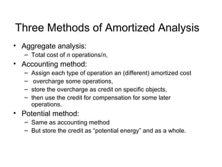
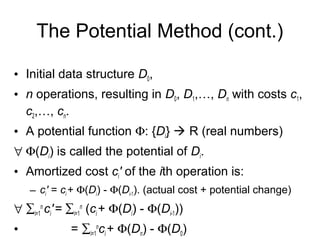
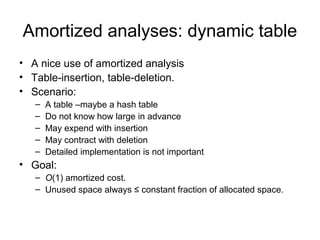
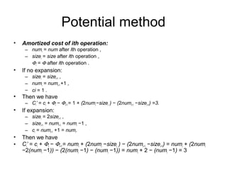
7. Amortized (Aggregate) Analysis of INCREMENT(A)
Observation: The running time determined by #flips
but not all bits flip each time INCREMENT is called.
A[0] flips every time, total n times.
A[1] flips every other time, n/2 times.
A[2] flips every forth time, n/4 times.
….
for i=0,1,…,k-1, A[i] flips n/2i
 times.
Thus total #flips is ∑i=0
k-1
n/2i

< n∑i=0
∞
1/2i
=2n.

8. Amortized Analysis of INCREMENT(A)
• Thus the worst case running time is O(n)
for a sequence of n INCREMENTs.
• So the amortized cost per operation is
O(1).

9. Amortized Analysis: Accounting Method
• Idea:
– Assign differing charges to different operations.
– The amount of the charge is called amortized cost.
– amortized cost is more or less than actual cost.
– When amortized cost > actual cost, the difference is
saved in specific objects as credits.
– The credits can be used by later operations whose
amortized cost < actual cost.
• As a comparison, in aggregate analysis, all
operations have same amortized costs.

10. Accounting Method (cont.)
• Conditions:
– suppose actual cost is ci for the ith operation in the
sequence, and amortized cost is ci',
– ∑i=1
n
ci' ≥∑i=1
n
ci should hold.
• since we want to show the average cost per
operation is small using amortized cost, we need the
total amortized cost is an upper bound of total actual cost.
• holds for all sequences of operations.
– Total credits is ∑i=1
n
ci' - ∑i=1
n
ci , which should be
nonnegative,
• Moreover, ∑i=1
t
ci' - ∑i=1
t
ci ≥0 for anyt>0.

11. Accounting Method: Stack Operations
• Actual costs:
– PUSH :1, POP :1, MULTIPOP: min(s,k).
• Let assign the following amortized costs:
– PUSH:2, POP: 0, MULTIPOP: 0.
• Similar to a stack of plates in a cafeteria.
– Suppose $1 represents a unit cost.
– When pushing a plate, use one dollar to pay the actual cost of the push and
leave one dollar on the plate as credit.
– Whenever POPing a plate, the one dollar on the plate is used to pay the actual
cost of the POP. (same for MULTIPOP).
– By charging PUSH a little more, do not charge POP or MULTIPOP.
• The total amortized cost for n PUSH, POP, MULTIPOP is O(n), thus O(1)
for average amortized cost for each operation.
• Conditions hold: total amortized cost ≥total actual cost, and amount of
credits never becomes negative.

12. Accounting method: binary counter
• Let $1 represent each unit of cost (i.e., the flip of one bit).
• Charge an amortized cost of $2 to set a bit to 1.
• Whenever a bit is set, use $1 to pay the actual cost, and
store another $1 on the bit as credit.
• When a bit is reset, the stored $1 pays the cost.
• At any point, a 1 in the counter stores $1, the number of 1’s
is never negative, so is the total credits.
• At most one bit is set in each operation, so the amortized
cost of an operation is at most $2.
• Thus, total amortized cost of n operations is O(n), and
average is O(1).

13. The Potential Method
• Same as accounting method:
something prepaid is used later.
• Different from accounting method
– The prepaid work not as credit, but as
“potential energy”, or “potential”.
– The potential is associated with the data
structure as a whole rather than with
specific objects within the data structure.

14. The Potential Method (cont.)
• Initial data structure D0,
• n operations, resulting in D0, D1,…, Dn with costs c1,
c2,…, cn.
• A potential function Φ: {Di}  R (real numbers)
∀ Φ(Di) is called the potential of Di.
• Amortized cost ci' of the ith operation is:
– ci' = ci + Φ(Di) - Φ(Di-1). (actual cost + potential change)
∀ ∑i=1
n
ci'= ∑i=1
n
(ci + Φ(Di) - Φ(Di-1))
• = ∑i=1
n
ci + Φ(Dn) - Φ(D0)

15. The Potential Method (cont.)
• If Φ(Dn) ≥ Φ(D0), then total amortized cost is an upper
bound of total actual cost.
• But we do not know how many operations, so Φ(Di) ≥
Φ(D0) is required for any i.
• It is convenient to define Φ(D0)=0,and so Φ(Di) ≥0, for all i.
• If the potential change is positive (i.e., Φ(Di) - Φ(Di-1)>0),
then ci' is an overcharge (so store the increase as
potential),
• otherwise, undercharge (discharge the potential to pay the
actual cost).

16. Potential method: stack operation
• Potential for a stack is the number of objects in the stack.
• So Φ(D0)=0, and Φ(Di) ≥0
• Amortized cost of stack operations:
– PUSH:
• Potential change: Φ(Di)- Φ(Di-1) =(s+1)-s =1.
• Amortized cost: ci' = ci + Φ(Di) - Φ(Di-1)=1+1=2.
– POP:
• Potential change: Φ(Di)- Φ(Di-1) =(s-1) –s= -1.
• Amortized cost: ci' = ci + Φ(Di) - Φ(Di-1)=1+(-1)=0.
– MULTIPOP(S,k): k'=min(s,k)
• Potential change: Φ(Di)- Φ(Di-1) = –k'.
• Amortized cost: ci' = ci + Φ(Di) - Φ(Di-1)=k'+(-k')=0.
• So amortized cost of each operation is O(1), and total amortized cost of n
operations is O(n).
• Since total amortized cost is an upper bound of actual cost, the worse case
cost of n operations is O(n).

17. Potential method: binary counter
• Define the potential of the counter after the ith INCREMENT is
Φ(Di) =bi, the number of 1’s. clearly, Φ(Di)≥0.
• Let us compute amortized cost of an operation
– Suppose the ith operation resets ti bits.
– Actual cost ci of the operation is at most ti +1.
– If bi=0, then the ith operation resets all k bits, so bi-1=ti=k.
– If bi>0, then bi=bi-1-ti+1
– In either case, bi≤bi-1-ti+1.
– So potential change is Φ(Di) - Φ(Di-1) ≤bi-1-ti+1-bi-1=1-ti.
– So amortized cost is: ci' = ci+ Φ(Di) - Φ(Di-1)≤ ti +1+1-ti=2.
• The total amortized cost of n operations is O(n).
• Thus worst case cost is O(n).

18. Amortized analyses: dynamic table
• A nice use of amortized analysis
• Table-insertion, table-deletion.
• Scenario:
– A table –maybe a hash table
– Do not know how large in advance
– May expend with insertion
– May contract with deletion
– Detailed implementation is not important
• Goal:
– O(1) amortized cost.
– Unused space always ≤ constant fraction of allocated space.

19. Dynamic table
• Load factor α = num/size, where num = #
items stored, size = allocated size.
• If size = 0, then num = 0. Call α = 1.
• Never allow α > 1.
• Keep α >a constant fraction  goal (2).

20. Dynamic table: expansion with insertion
• Table expansion
• Consider only insertion.
• When the table becomes full, double its
size and reinsert all existing items.
• Guarantees that α ≥ 1/2.
• Each time we actually insert an item into
the table, it’s an elementary insertion.

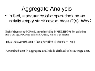
21. Copyright © The McGraw-Hill Companies, Inc. Permission required for reproduction or display.
Num[t] ele. insertion
1 ele. insertion
Initially, num[T ] = size[T ] = 0.

22. Aggregate analysis
• Running time: Charge 1 per elementary insertion. Count only
elementary insertions,
• since all other costs together are constant per call.
• ci = actual cost of ith operation
– If not full, ci = 1.
– If full, have i − 1 items in the table at the start of the ith operation. Have
to copy all i − 1 existing items, then insert ith item, ⇒ ci = i
• Cursory analysis: n operations ⇒ ci = O(n) ⇒ O(n2
) time for n
operations.
• Of course, we don’t always expand:
– ci = i if i − 1 is exact power of 2 ,
1 otherwise .
• So total cost =∑i=1
n
ci ≤n+ ∑i=0
log(n)
2i
≤n+2n=3n
• Therefore, aggregate analysis says amortized cost per operation =
3.

23. Accounting analysis
• Charge $3 per insertion of x.
– $1 pays for x’s insertion.
– $1 pays for x to be moved in the future.
– $1 pays for some other item to be moved.
• Suppose we’ve just expanded, size = m before next expansion, size
= 2m after next expansion.
• Assume that the expansion used up all the credit, so that there’s no
credit stored after the expansion.
• Will expand again after another m insertions.
• Each insertion will put $1 on one of the m items that were in the
table just after expansion and will put $1 on the item inserted.
• Have $2m of credit by next expansion, when there are 2m items to
move. Just enough to pay for the expansion, with no credit left over!

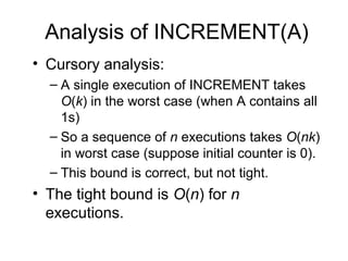
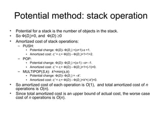
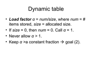
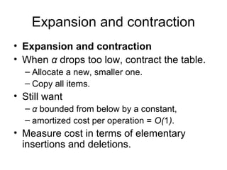
24. Potential method
• Potential method
∀ Φ(T ) = 2 ・ num[T ] − size[T ]
• Initially, num = size = 0⇒ Φ = 0.
• • Just after expansion, size = 2 ・ num ⇒ Φ =
0.
• Just before expansion, size = num ⇒ Φ = num
⇒ have enough potential to pay for moving all
items.
• Need Φ ≥ 0, always.
• Always have
– size ≥ num ≥ ½ size ⇒ 2 ・ num ≥ size ⇒ Φ ≥ 0 .

25. Potential method
• Amortized cost of ith operation:
– numi = num after ith operation ,
– sizei = size after ith operation ,
Φi = Φ after ith operation .
• If no expansion:
– sizei = sizei−1 ,
– numi = numi−1 +1 ,
– ci = 1 .
• Then we have
– Ci’ = ci + Φi − Φi−1 = 1 + (2numi −sizei ) − (2numi−1 −sizei−1) =3.
• If expansion:
– sizei = 2sizei−1 ,
– sizei−1 = numi−1 = numi −1 ,
– ci = numi−1 +1 = numi.
• Then we have
• Ci’ = ci + Φi − Φi−1 = numi + (2numi −sizei ) − (2numi−1 −sizei−1) = numi + (2numi
−2(numi −1)) − (2(numi −1) − (numi −1)) = numi + 2 − (numi −1) = 3

26. Copyright © The McGraw-Hill Companies, Inc. Permission required for reproduction or display.

27. Expansion and contraction
• Expansion and contraction
• When α drops too low, contract the table.
– Allocate a new, smaller one.
– Copy all items.
• Still want
– α bounded from below by a constant,
– amortized cost per operation = O(1).
• Measure cost in terms of elementary
insertions and deletions.

28. Obvious strategy
• Double size when inserting into a full table (when α = 1, so that after
insertion α would become <1).
• Halve size when deletion would make table less than half full (when
α = 1/2, so that after deletion α would become >= 1/2).
• Then always have 1/2 ≤ α ≤ 1.
• Suppose we fill table.
– Then insert ⇒ double
– 2 deletes ⇒ halve
– 2 inserts ⇒ double
– 2 deletes ⇒ halve
– ・ ・ ・
– Cost of each expansion or contraction is Θ(n), so total n operation will
be Θ(n2
).
• Problem is that: Not performing enough operations after expansion
or contraction to pay for the next one.

29. Simple solution
• Double as before: when inserting with α = 1 ⇒ after doubling, α = 1/2.
• Halve size when deleting with α = 1/4 ⇒ after halving, α = 1/2.
• Thus, immediately after either expansion or contraction, have α = 1/2.
• Always have 1/4 ≤ α ≤ 1.
• Intuition:
• Want to make sure that we perform enough operations between
consecutive expansions/contractions to pay for the change in table
size.
• Need to delete half the items before contraction.
• Need to double number of items before expansion.
• Either way, number of operations between expansions/contractions is
at least a constant fraction of number of items copied.

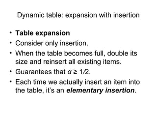
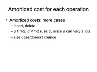
30. Potential function
∀Φ(T) = 2num[T] − size[T] if α ≥ ½
size[T]/2 −num[T] ifα < ½ .
• T empty ⇒ Φ = 0.
• α ≥ 1/2 ⇒ num ≥ 1/2size ⇒ 2num ≥ size
⇒ Φ ≥ 0.
• α < 1/2 ⇒ num < 1/2size ⇒ Φ ≥ 0.

31. intuition
• measures how far from α = 1/2 we are.
– α = 1/2 ⇒ Φ = 2num−2num = 0.
– α = 1 ⇒ Φ = 2num−num = num.
– α = 1/4 ⇒ Φ = size /2 − num = 4num /2 − num = num.
• Therefore, when we double or halve, have enough potential to pay for
moving all num items.
• Potential increases linearly between α = 1/2 and α = 1, and it also increases
linearly between α = 1/2 and α = 1/4.
• Since α has different distances to go to get to 1 or 1/4, starting from 1/2,
rate of increase differs.
• For α to go from 1/2 to 1, num increases from size /2 to size, for a total
increase of size /2. Φ increases from 0 to size. Thus, Φ needs to increase
by 2 for each item inserted. That’s why there’s a coefficient of 2 on the
num[T ] term in the formula for when α ≥ 1/2.
• For α to go from 1/2 to 1/4, num decreases from size /2 to size /4, for a total
decrease of size /4. Φ increases from 0 to size /4. Thus, Φ needs to
increase by 1 for each item deleted. That’s why there’s a coefficient of −1 on
the num[T ] term in the formula for when α < 1/2.

32. • Amortized costs: more cases
– insert, delete
– α ≥ 1/2, α < 1/2 (use αi, since α can vary a lot)
– size does/doesn’t change
Amortized cost for each operation

33. Splay tree
• A binary search tree (not balanced)
• Height may be larger than log n, even n-1.
• However a sequence of n operations takes O(nlog n).
• Assumptions: data values are distinct and form a totally
order set
• Operations:
– Member(i,S)
– Insert(i,S)
– Delete(i,S)
– Merge(S,S’)
– Split(i,S)
– All based on
• splay(i,S), reorganize tree so that i to be root if i∈S, otherwise, the
new root is either max{k ∈S |k<i} or min{k ∈S |k>i}

34. Splay tree (cont.)
• For examples,
– merge(S,S’)
• Call Splay(∞, S) and then make S’ the right child
– Delete(i,S), call Splay(i,S), remove I, then
merge(left(i), right(i)).
– Similar for others.
– Constant number of splays called.

35. Splay tree (cont.)
• Splay operation is based on basic
rotate(x) operation (either left or right).
• Three cases:
– y is the parent of x and x has not grandparent
• rotate(x)
– x is the left (or right) child of y and y is the left
(or right) child of z,
• rotate(y) and then rotate(x)
– x is the left (or right) child of y and y is the
right (or left) child of z,
• rotate(x) and then rotate(x)

36. Splay tree (cont.)
• Credit invariant: Node x always has at
least log µ(x) credits on deposit.
– Where µ(S)=log (|S|) and µ(x)=µ(S(x))
• Lemma:
– Each operation splay(x,S) requires no more
than 3(µ(S)-µ(x))+1 credits to perform the
operation and maintain the credit invariant.
• Theorem:
– A sequence of m operations involving n inserts
takes time O(mlog(n)).

37. Summary
• Amortized analysis
– Different from probabilistic analysis
• Three methods and their differences
• how to analyze