Download to read offline
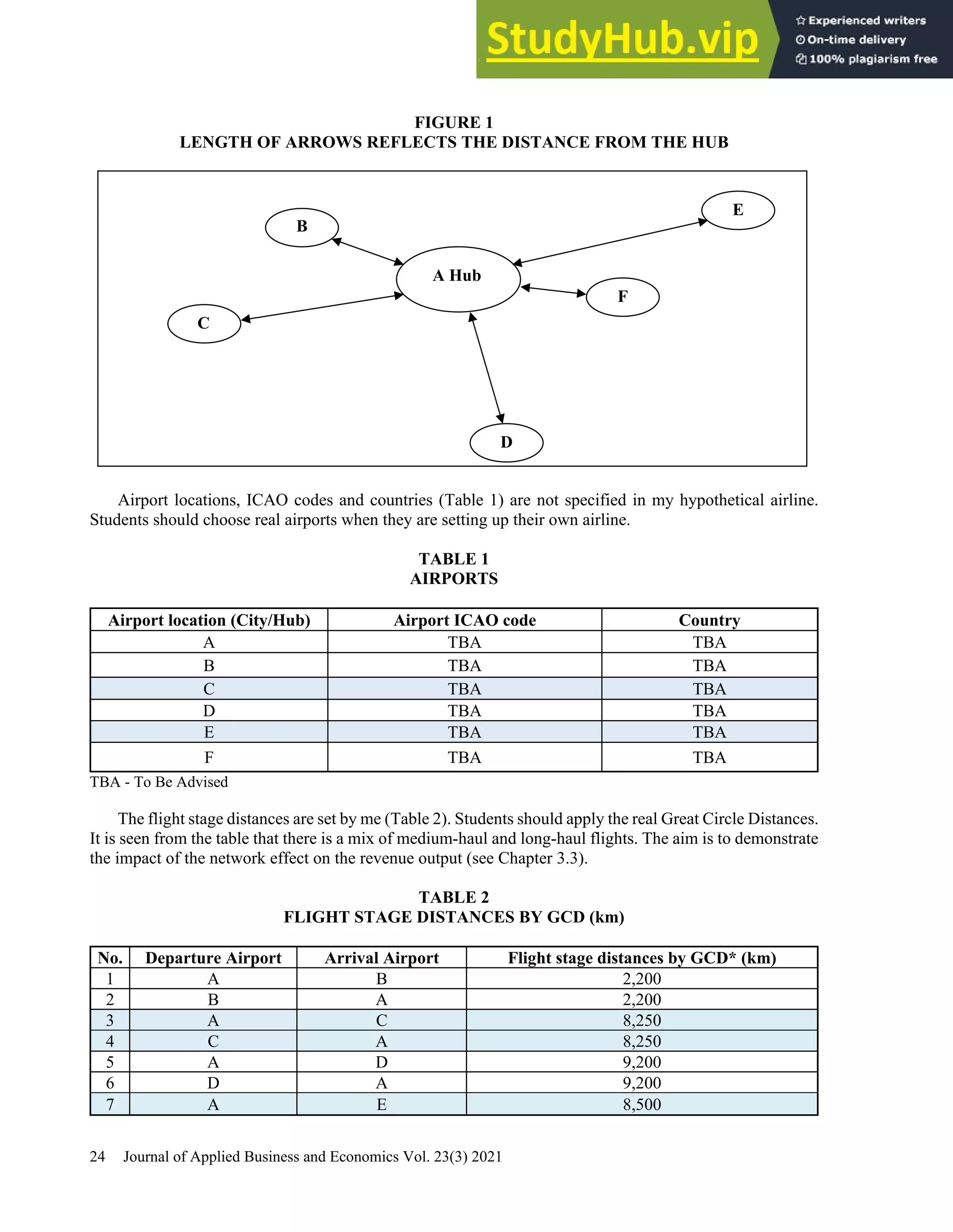
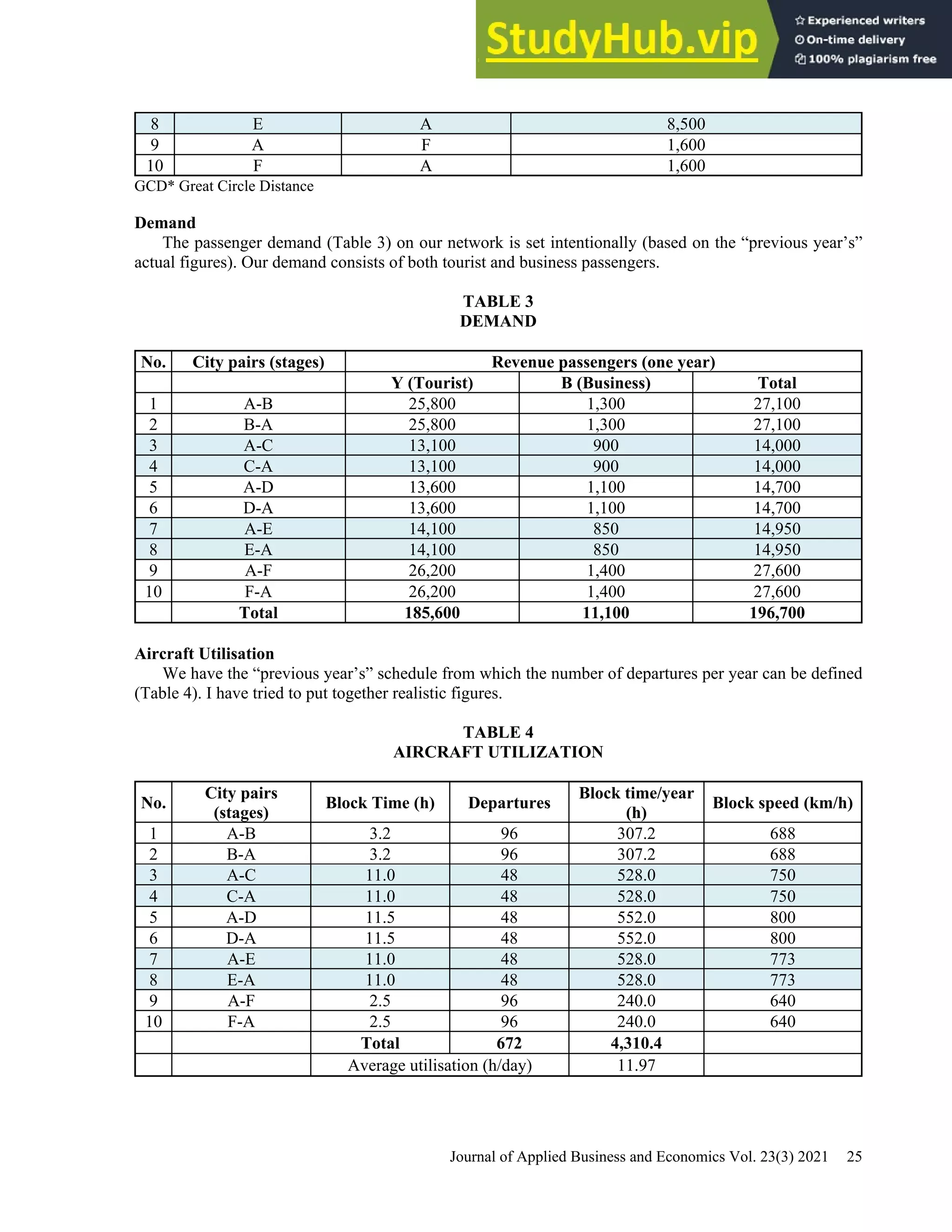
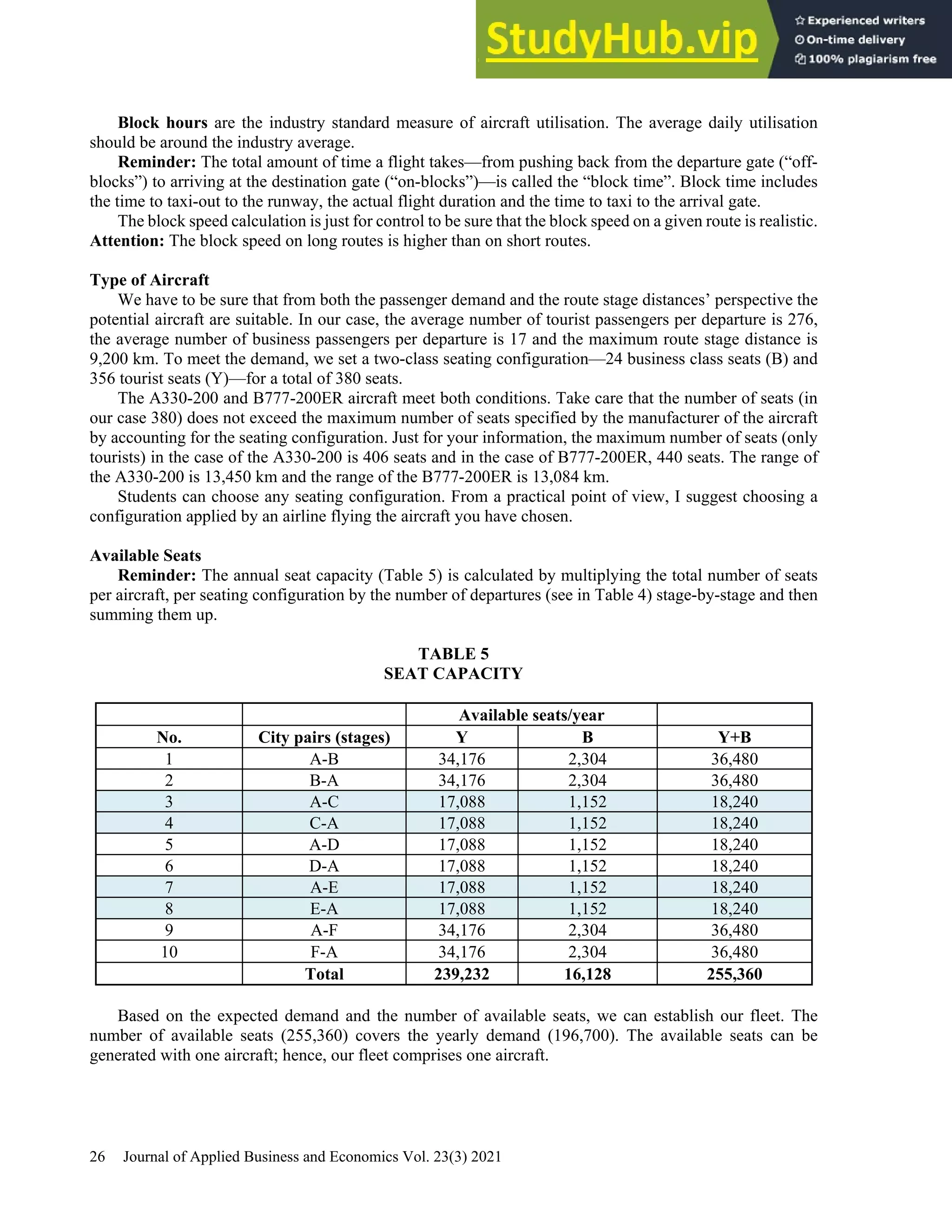
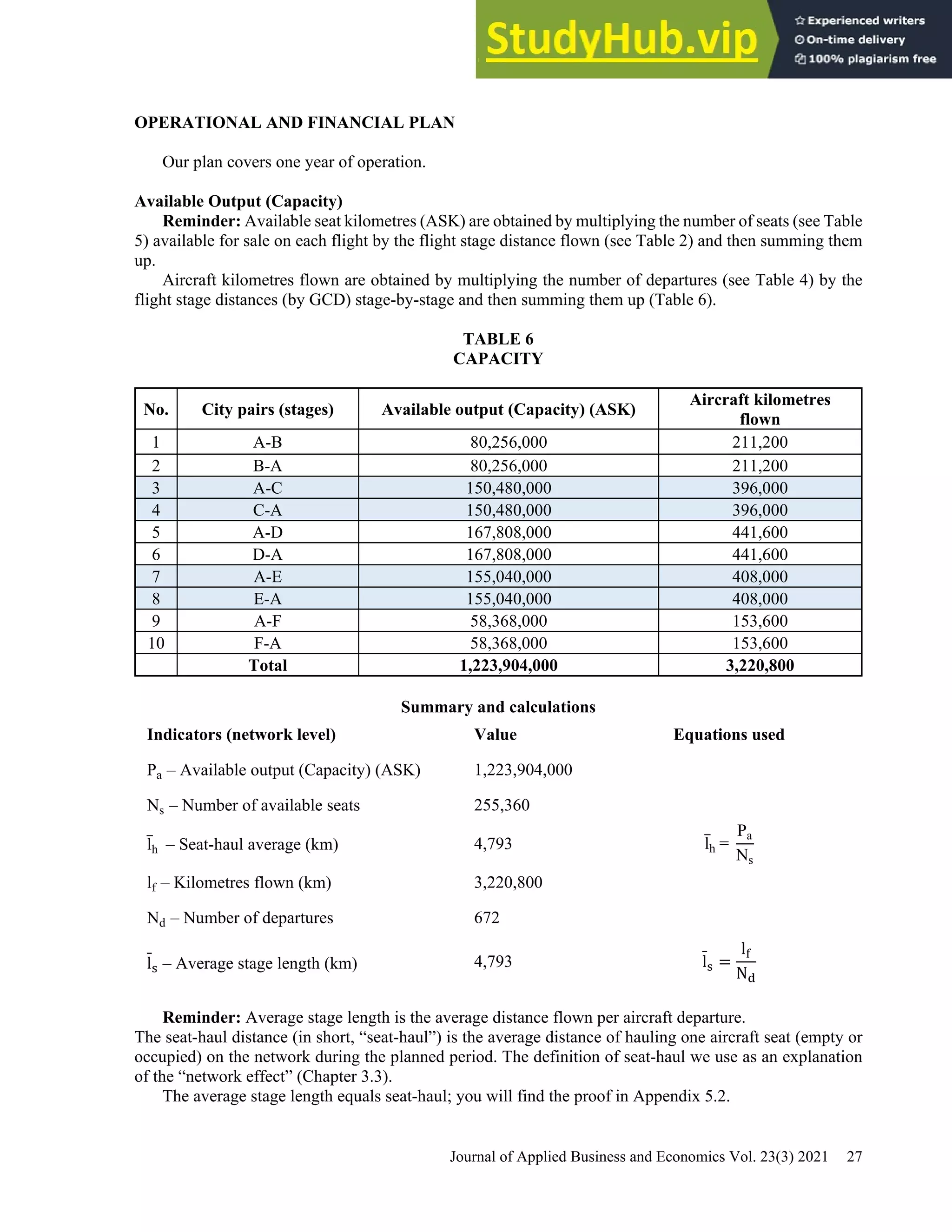
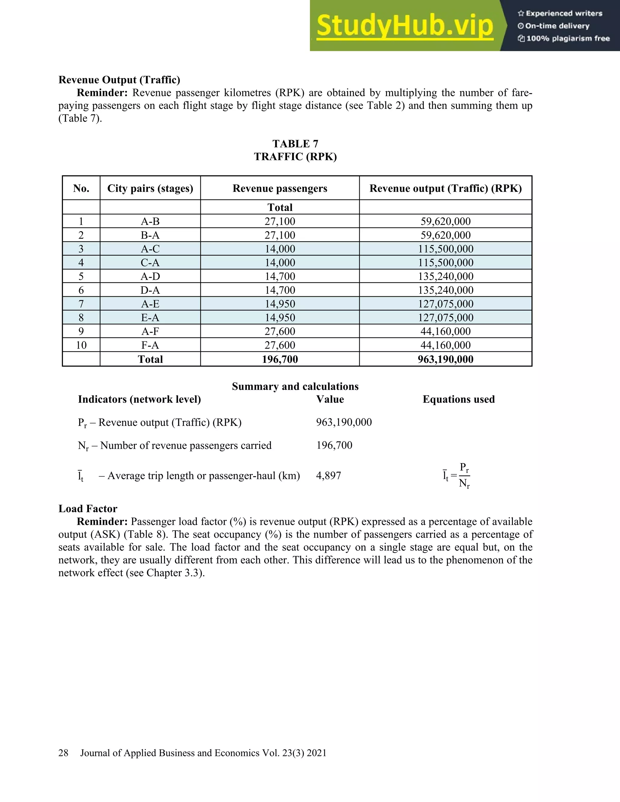
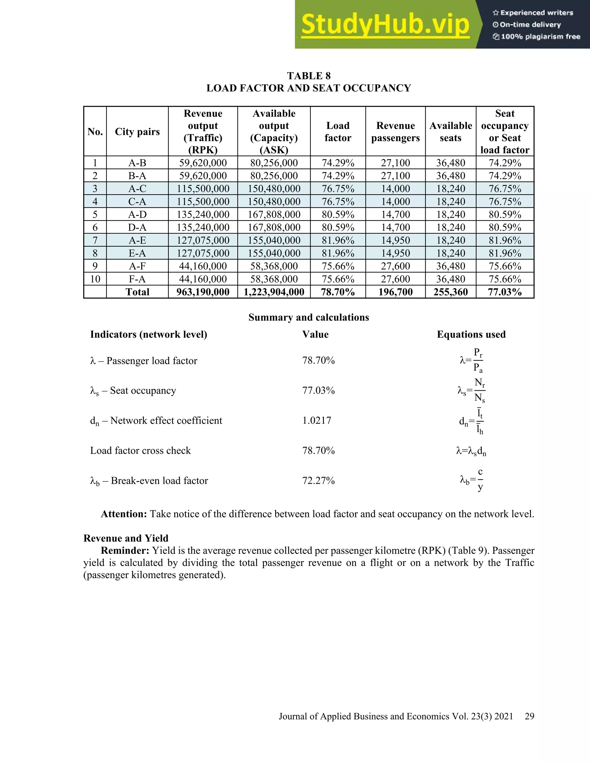
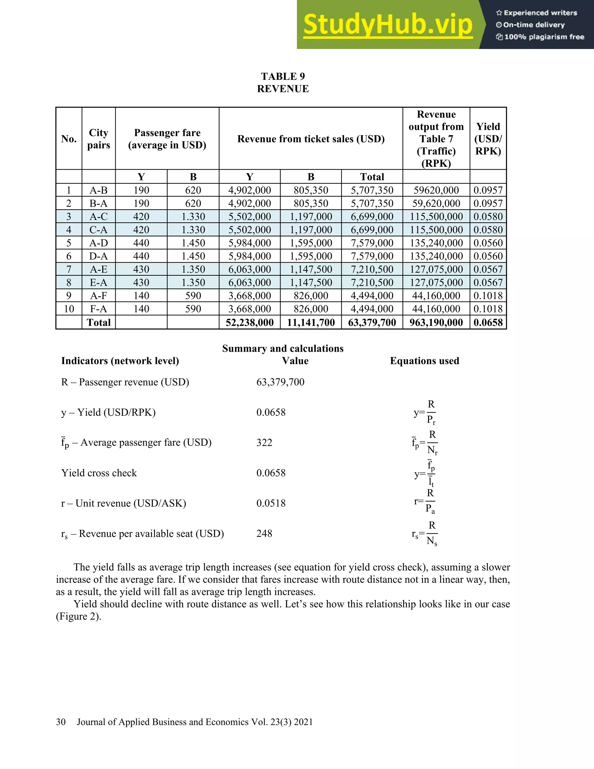
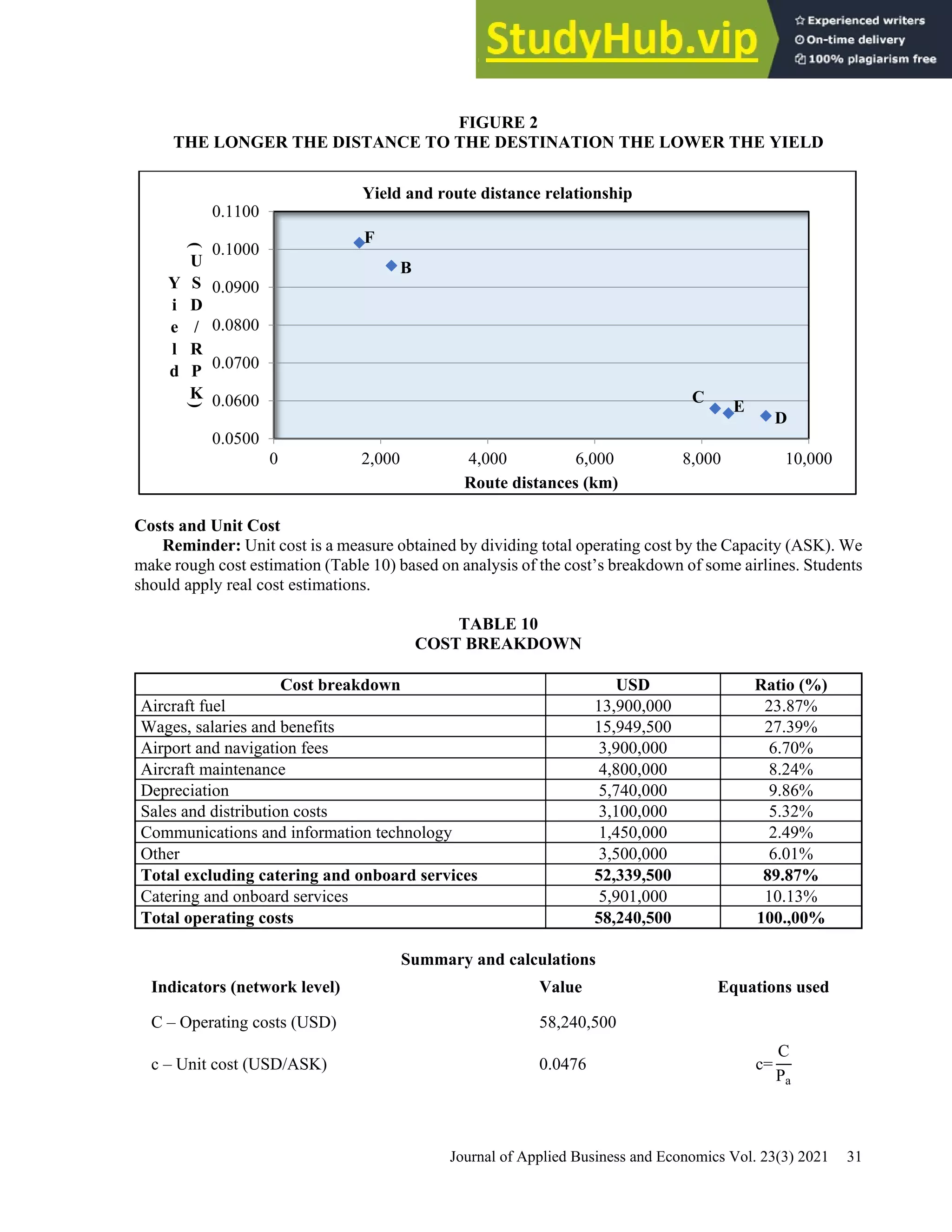
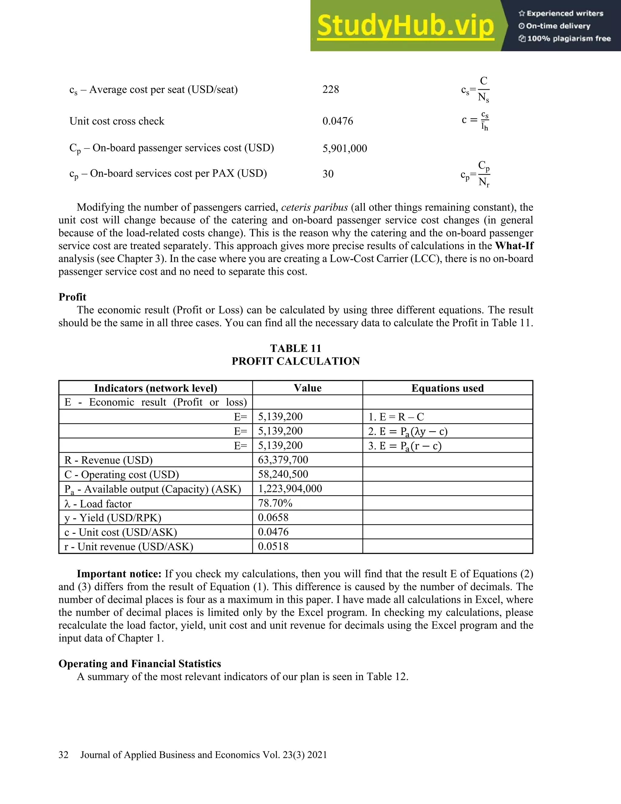
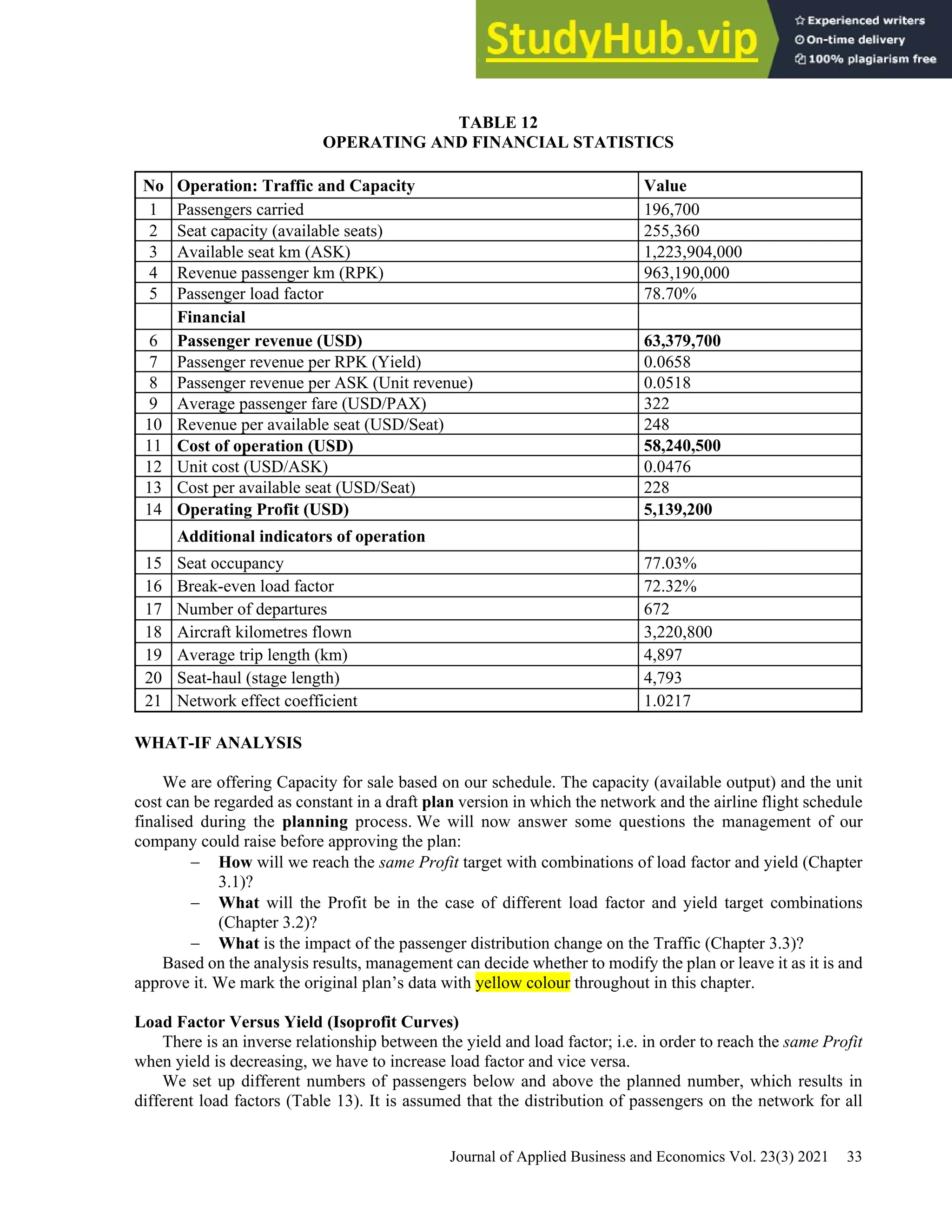
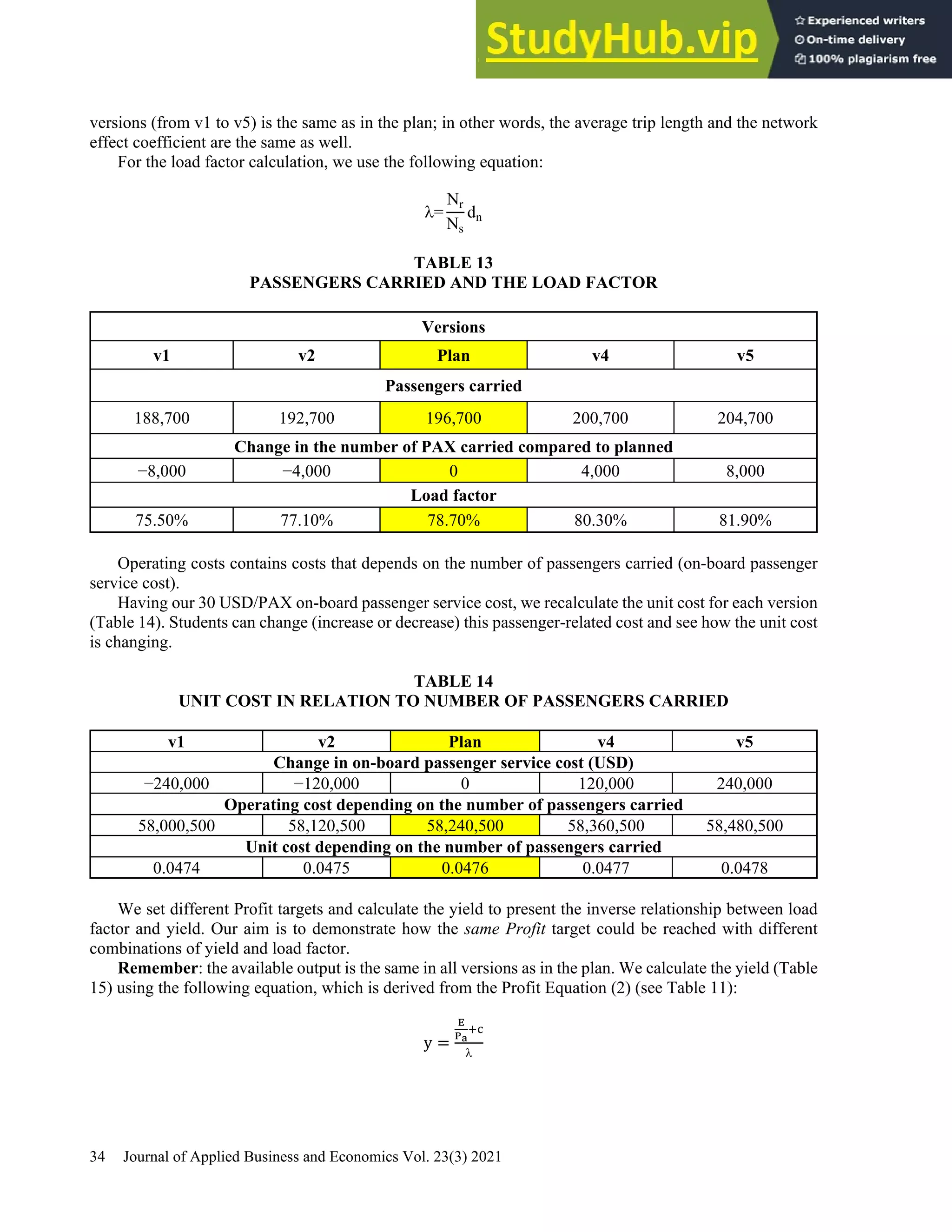
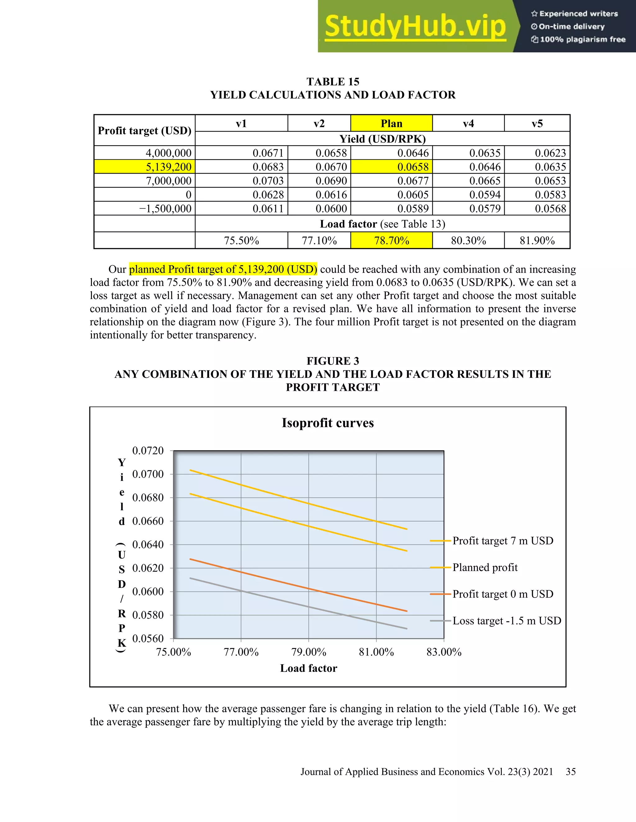
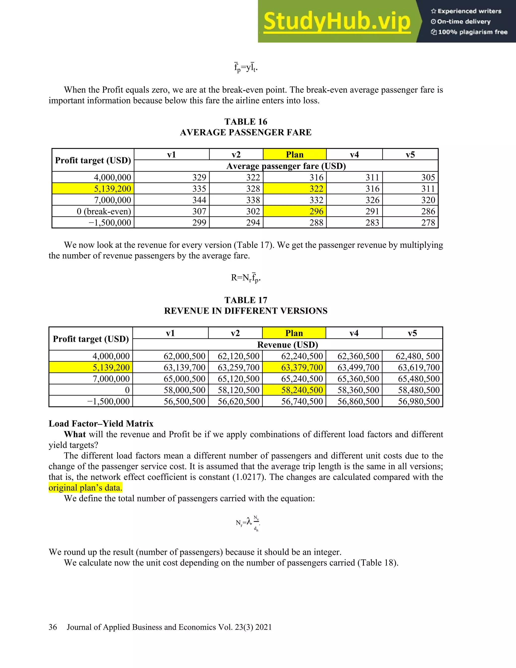
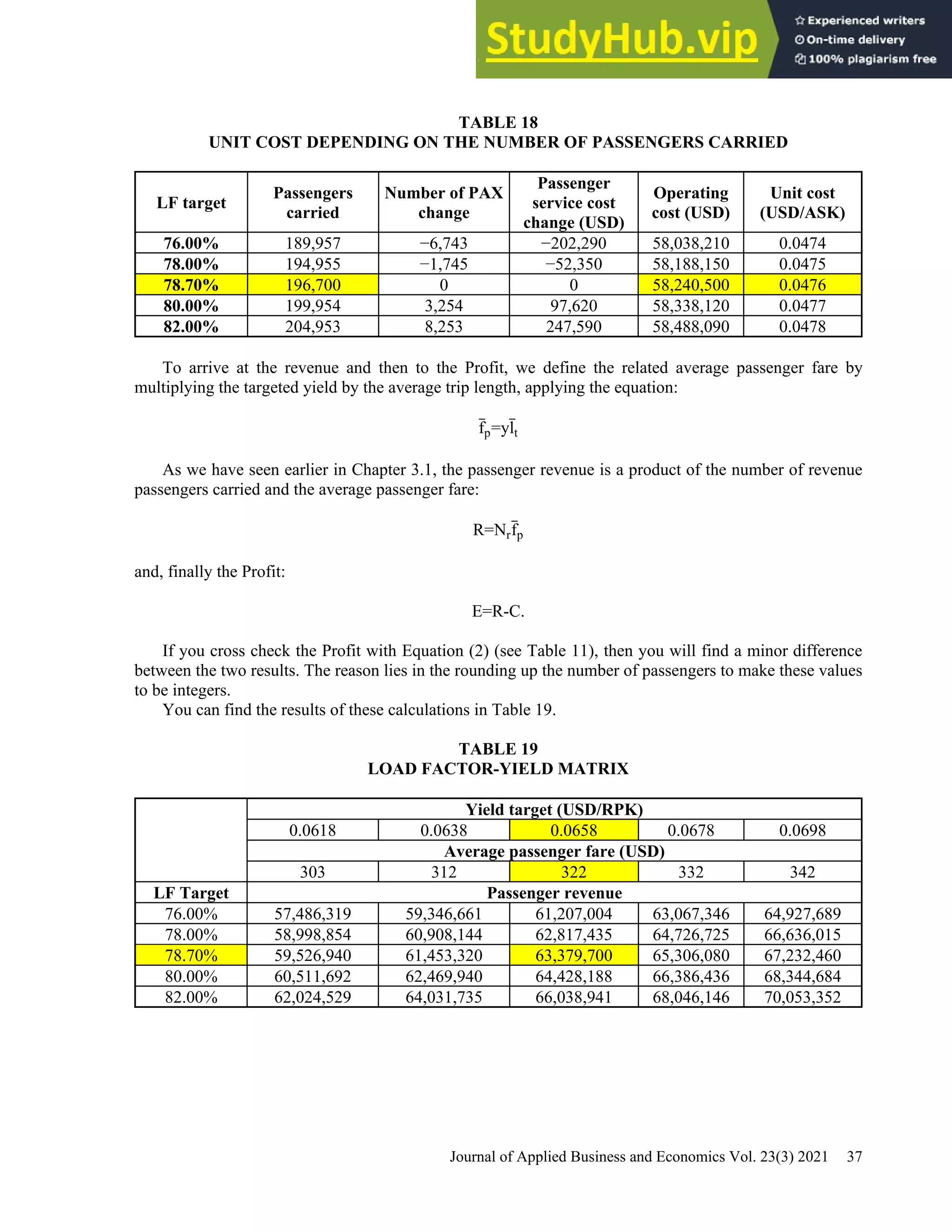
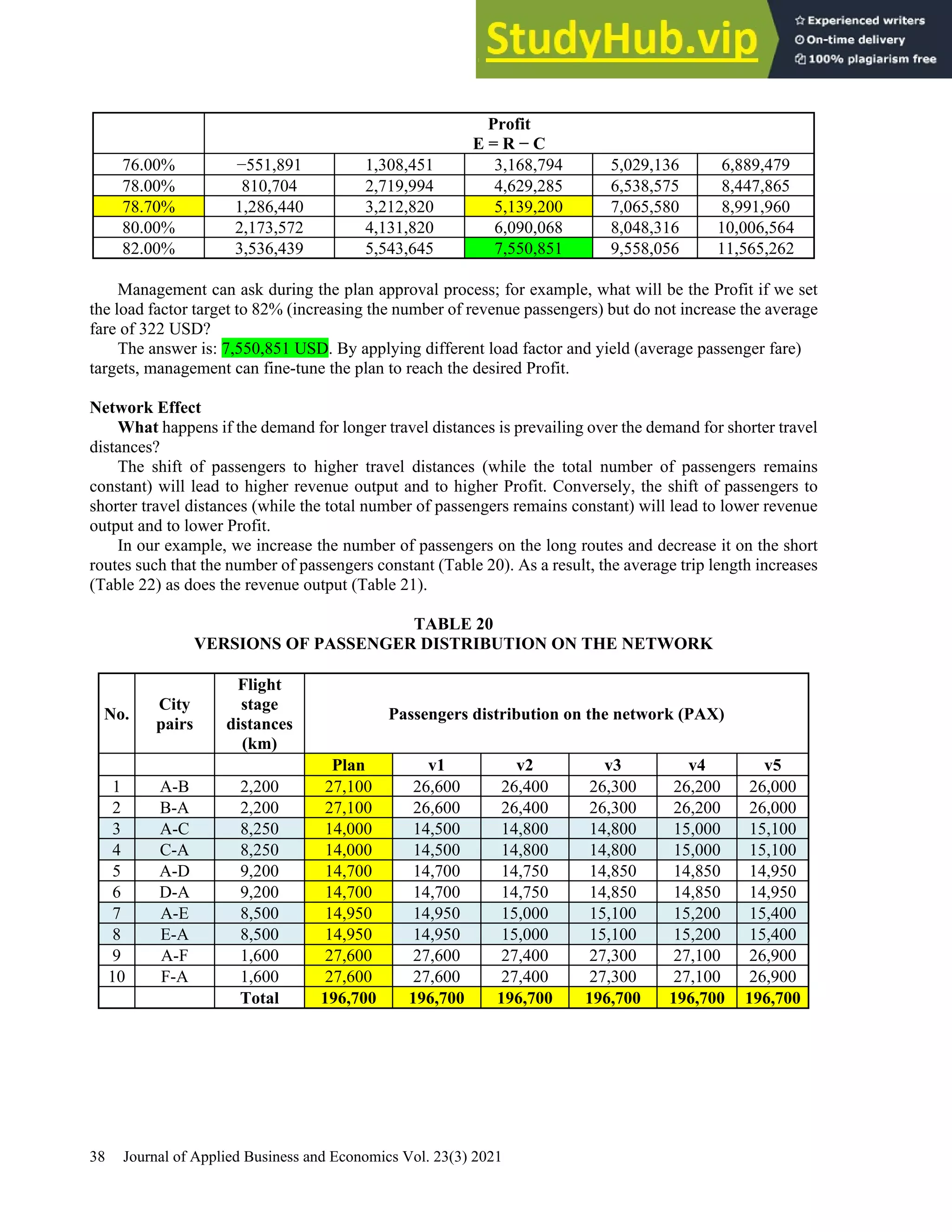

This document provides a practical guide for students to understand key performance indicators of airline economics. It sets up a hypothetical airline called "MyAir" with a simple hub-and-spoke network connecting 6 airports. Demand data and aircraft utilization are estimated to develop a one-year operational plan. A fleet of one aircraft, either an Airbus A330-200 or Boeing 777-200ER, is determined to meet the estimated annual demand of 196,700 passengers. The guide is intended for classroom discussion and demonstrates relationships between profit drivers like load factor, yield, and unit cost through a "what-if" analysis.


