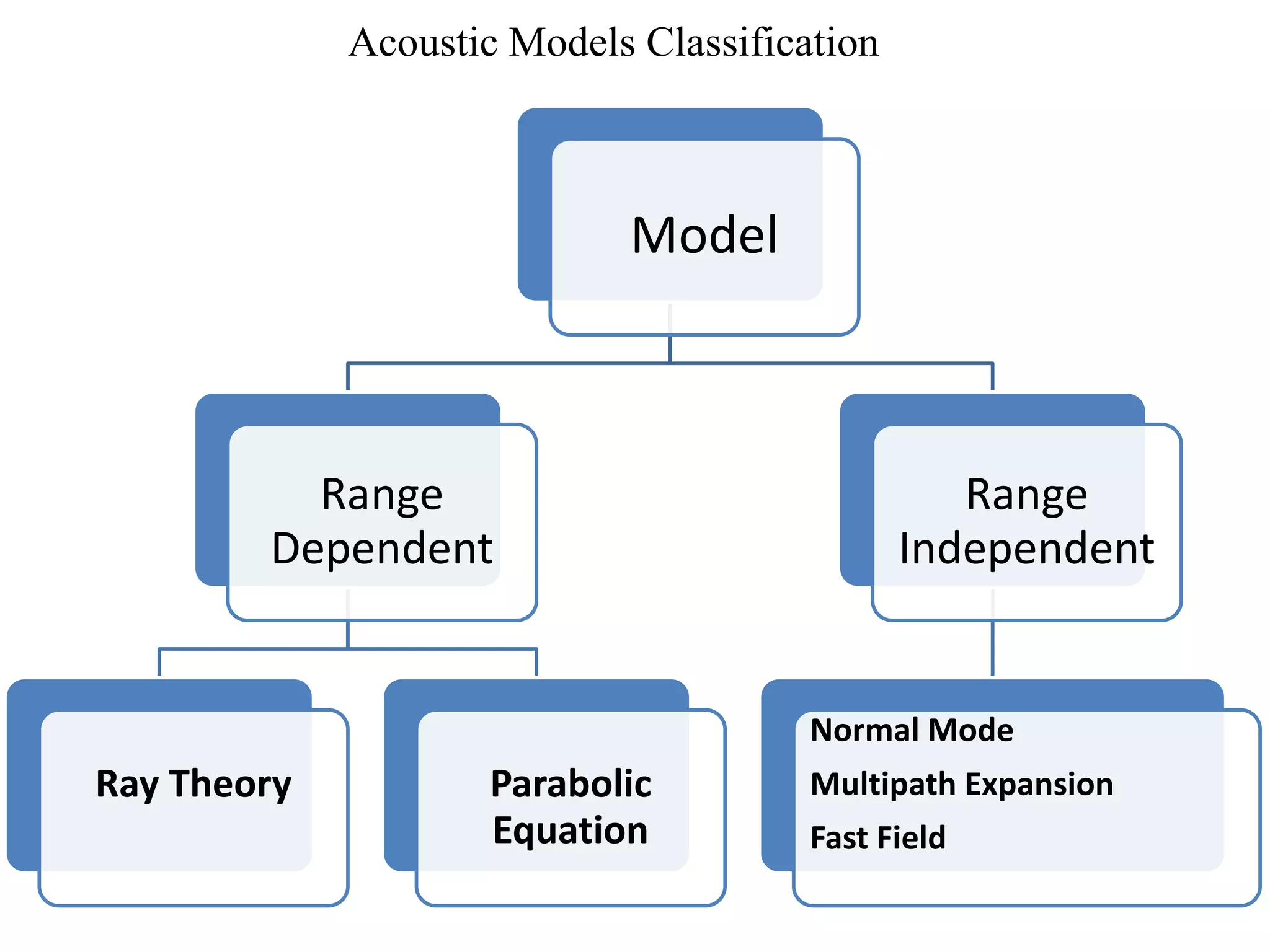
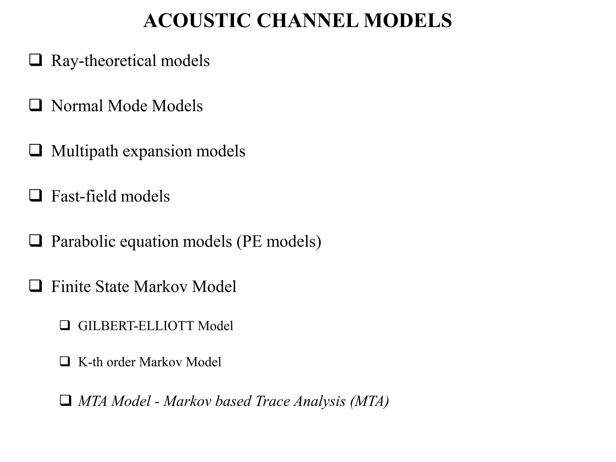
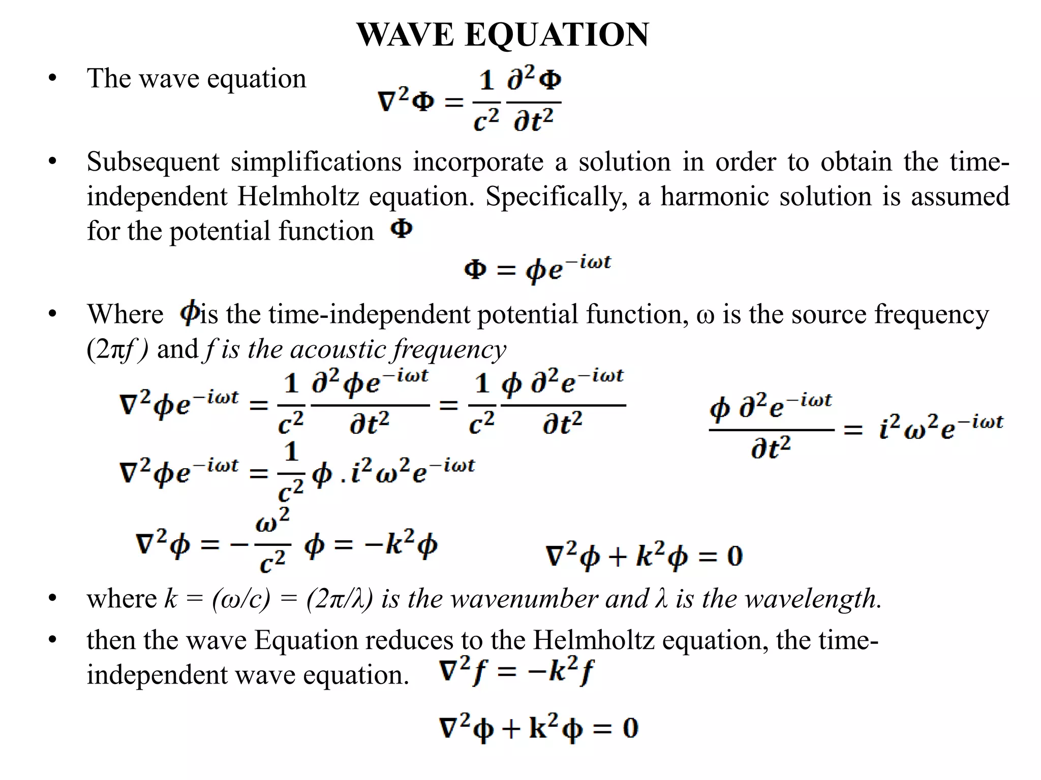
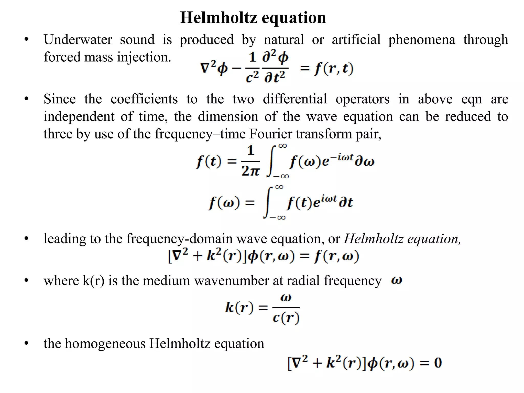
The document discusses acoustic modeling techniques for underwater sound propagation. It provides an overview of several common modeling approaches, including ray theory models, normal mode models, multipath expansion models, fast field models, and parabolic equation models. It also discusses how these approaches relate to solving the acoustic wave equation and Helmholtz equation. The key steps of ray theory modeling are outlined, including derivation of the eikonal and transport equations from the Helmholtz equation.

1. Acoustic Model

2. Acoustic Models Classification
Model
Range
Dependent
Ray Theory Parabolic
Equation
Range
Independent
Normal Mode
Multipath Expansion
Fast Field

3. Ray Theory Model
• BELLHOP gaussian beam/finite element beam code(2018)
(M. Porter, Heat, Light, and Sound Research, Inc.)
• Eigenray Eigenray Acoustic Ray Tracing Code (2015)
(B. Dushaw, Applied Physics Laboratory, U. Washington)
• TRACEO Beam Tracing code (2015)
(O. Rodríguez and Emanuel Ey, Univ. Algarve, Portugal)
• HWT_3D_mm Huygens Wavefront Tracing in 3D for moving media (2013)
(Nikolay Zabotin, Oleg A. Godin, and Liudmila Ye. Zabotina, National Oceanic and Atmospheric
Administration)
• USML: Under Sea Modeling Library with WaveQ3D beam tracing code for 3D (C++) (2015) (S.
Reilly, Univ. Rhode Island and AEgis Technologies Group)
• TV-APM: Time-Variable Acoustic Propagation Model (manual) (2012)
(A. J. Silva and O. Rodríguez, University of Algarve, Portugal)
• Ray, Eigenray Ray Tracing Code (1992)
(Jim Bowlin, Orig. WHOI)A basic, easy to use, range-dependent

4. Normal Mode Model
• The KRAKEN Normal Mode Program (DRAFT)
Michael B. Porter
• KrakenZ: This version uses a new root finder based on winding number
integrals that is much more robust (P. Cristini /CNRS-Laboratoire de
Mécanique ed d'Acoustique, France)
Fast-Field Programs Model
• The SCOOTER FFP model - SCOOTER is a finite element code for
computing acoustic fields in range-independent environments.
• The SPARC pulse model - SPARC (SACLANTCEN Pulse Acoustic Research
Code) is an experimental time-marched FFP
• The BOUNCE reflection coefficient model - BOUNCE computes the
reflection coefficient for a stack of acoustic media optionally overlying elastic
media.

5. Parabolic Equation Models
• FOR3D : 3D and 2D PE model (this version is from L. Henderson, HLS with minor
fixes) (Feb. 14, 2015)
• MPIRAM: (Message Passing Interface) A parallel version of RAM that uses either
OPENMP or MPI for parallelization. (fortran 90) (B. Dushaw, Applied Physics
Laboratory, U. Washington)) (2015)
• RAMSurf - Range-dependent Acoustic Model : RAMSurf recoded in C and vectorized
for speed (Thomas Folegot, Quiet-Oceans); also on github repository (2013)
• MMPE : Monterey-Miami PE model and intro file. (K.B. Smith/U.S. Naval
Postgraduate School and F. Tappert/Rosenstiel School of Marine and Atmospheric
Sciences)
Updated 2006 to correct for treatment of attenuation and add calculations of the particle
velocity field
• UMPE : University of Miami PE model and User's Guide (the guide is also an excellent
introduction to the PE approach) (K. Smith and F. Tappert) (1998)

6. Simulators
Tools Year Language Propagation Model
S
i
m
u
l
a
t
i
o
n
T
o
o
l
NS-2 1996 C++ Radio Model
QualNet Visual C++ Radio Model
AUNetSim 2008 Python Thorp’s Model
WOSS 2009 C++ Bellhop, Kraken, Scooter,
SPARC
OPNET C++/Python Customized /
Pipeline Stages
Aqua-Sim 2009 C++ Thorp’s Model
Aqua-Tools 2009 C++ Thorp’s Model
Fisher-Simmons
Ainslie and McColm
Aqua-GLomo 2012 PARSEC Thorp’s Model
NS-3 2008 C++ / Python UAN Model

7. ACOUSTIC CHANNEL MODELS
 Ray-theoretical models
 Normal Mode Models
 Multipath expansion models
 Fast-field models
 Parabolic equation models (PE models)
 Finite State Markov Model
 GILBERT-ELLIOTT Model
 K-th order Markov Model
 MTA Model - Markov based Trace Analysis (MTA)

8. WAVE EQUATION
• The wave equation is itself derived from the more fundamental equations of state,
continuity and motion.
• Where is the Laplacian operator,
• is the potential function,
• c is the speed of sound and
• t is the time.
• the Laplace operator or Laplacian is a differential operator given by the divergence of
the gradient of a scalar function on Euclidean space.
• General Wave Equation

9. Derivation of WAVE EQUATION
• We take A as the origin, the line of equilibrium of the string as X Axis and the motion is
confirmed to XY Plane.
• Consider the motion the of an element PQ of length x
• Let P be at the distance x and Q be at the distance x+ x from A
• Let the tangents P and Q make angles 1 and 2 with the x-axis
• The vertical component of the force acting on element PQ is
• When is very small
• The vertical component of the force
• Newtons Law of Motion is F=MassXAcceleration
• From 1 & 2

10. Derivation of WAVE EQUATION
• When Q  P or x  0
• Finally by Rewriting

11. WAVE EQUATION
• The wave equation
• Subsequent simplifications incorporate a solution in order to obtain the time-
independent Helmholtz equation. Specifically, a harmonic solution is assumed
for the potential function
• Where is the time-independent potential function, ω is the source frequency
(2πf ) and f is the acoustic frequency
• where k = (ω/c) = (2π/λ) is the wavenumber and λ is the wavelength.
• then the wave Equation reduces to the Helmholtz equation, the time-
independent wave equation.

12. WAVE EQUATION
• In cylindrical coordinates, the above equation becomes -elliptic-reduced wave
equation.
• Throughout the theoretical development of these five techniques, the potential
function ϕ normally represents the acoustic field pressure. When this is the
case, the transmission loss (TL) can easily be calculated as
• To describe the different approaches effectively, it is useful to first develop a
classification scheme, with associated taxonomy, based on five canonical
solutions to the wave equation: ray theory, normal mode, multipath expansion,
fast field, and parabolic equation (PE) techniques.
• A generalized classification scheme has been constructed using five categories
or responding to the five canonical solutions of the wave equation

13. Classification Of Modeling Techniques

14. Helmholtz equation
• Underwater sound is produced by natural or artificial phenomena through
forced mass injection.
• Since the coefficients to the two differential operators in above eqn are
independent of time, the dimension of the wave equation can be reduced to
three by use of the frequency–time Fourier transform pair,
• leading to the frequency-domain wave equation, or Helmholtz equation,
• where k(r) is the medium wavenumber at radial frequency
• the homogeneous Helmholtz equation

15. RAY-THEORY MODEL
• Our starting point is the Helmholtz equation in Cartesian coordinates x =(x, y,
z)
• where c.x/ is the sound speed and ! is the angular frequency of the source
located at x0. To obtain the ray equations, we seek a solution of the Helmholtz
equation in the form
• This is called the ray series. Taking derivatives of the ray series, we obtain

16. RAY-THEORY MODEL
• Thus, we can write
• Substituting this result into the Helmholtz equation and equating terms of like
order in ,we obtain the following infinite sequence of equations for the
functions and
• The equation for is known as the eikonal equation. The remaining
equations for are known as the transport equations.

17. RAY-THEORY MODEL
Eikonal Equation: The eikonal equation is a first-order nonlinear PDE that can be
solved by a variety of techniques.
Since is a vector perpendicular to the wavefronts, we can define the ray
trajectory x(s) by the following differential equation,
• The factor of c is introduced so that the tangent vector dx/ds has unit length.
Now, from the eikonal equation the term on the right is found to be unity.
Since dx/ds =1, the parameter s is simply the arclength along the ray.
Differentiation with respect to s yields

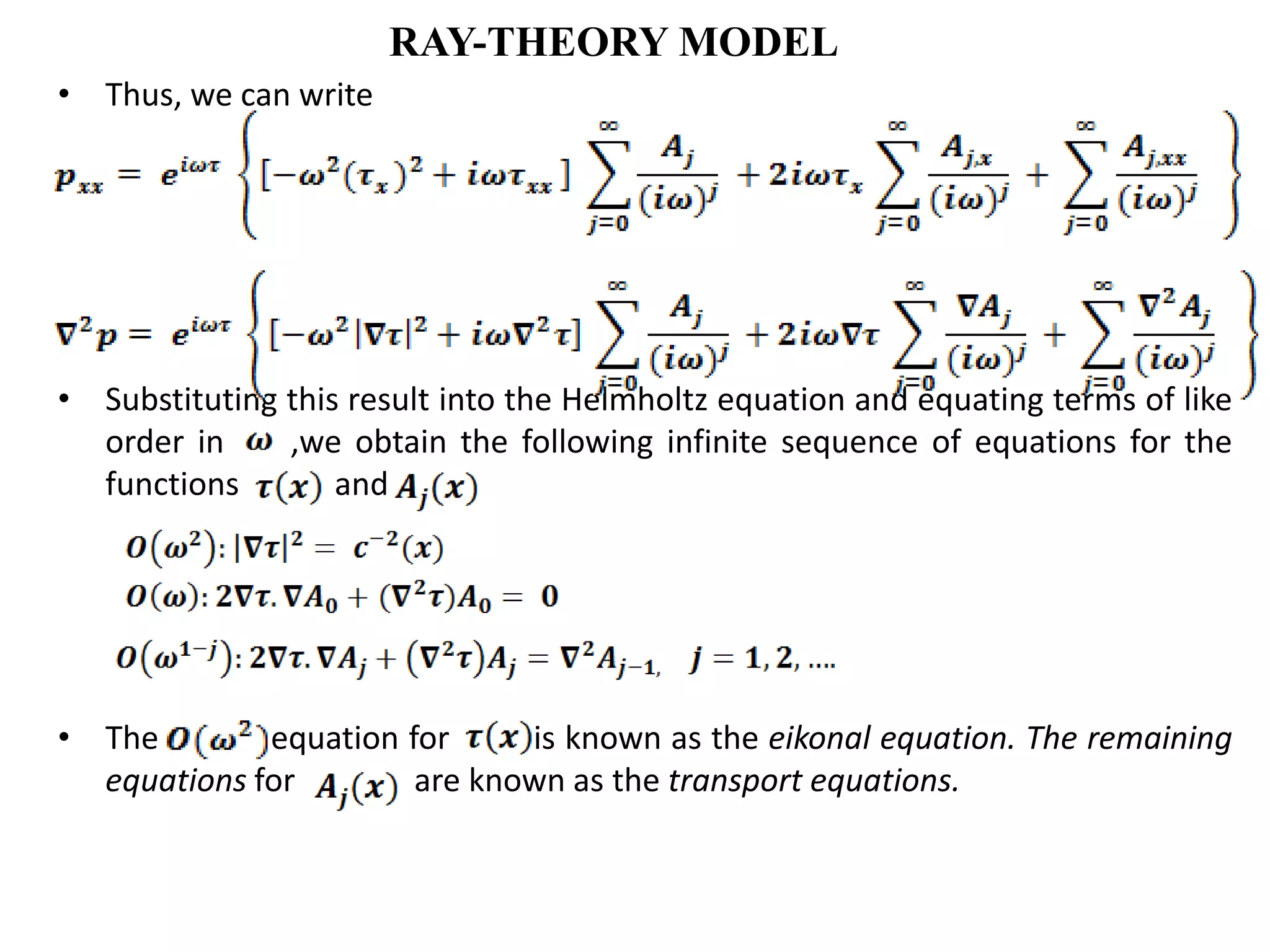
18. RAY-THEORY MODEL
Using this can be written as
Then, using the eikonal equation, to replace the terms in square brackets, we
Obtain
By applying this process to each of the coordinates, we obtain the following
vector equation for the ray trajectories,
In cylindrical coordinates (r,z), these ray equations may be written in the first-
order form
where [r(s), z(s)] is the trajectory of the ray in the range–depth plane. We have
introduced the auxiliary variables and in order to write the equations in
first-order form.

19. RAY-THEORY MODEL
Recall that the tangent vector to a curve [r(s), z(s)] parameterized by arc length is
given by [dr/ds, dz/ds]. Thus, from the above equations the tangent vector to the
ray is
normal vectors to the ray:
One may immediately verify that tray .nray =0. The tangent and normal are, of
course, arbitrary with respect to sign. However, to complete the specification of
the rays we also need initial conditions.
As indicated in Fig. 3.3, the initial conditions are that the ray starts at the source
position [ro, zo] with a specified take-off angle . Thus, we have

20. RAY-THEORY MODEL
To obtain the pressure field we need to associate a phase and an amplitude with
each ray. The phase is obtained by solving the eikonal equation in the coordinate
systemof the rays. Recall that
Therefore
This is the eikonal equation written in terms of the ray coordinate s. Note that the
original nonlinear PDE has been reduced to a linear ordinary differential equation
which is readily solved to yield
The integral term in this equation is the travel time along the ray, so from a
physical point of view the phase of the wave is simply delayed in accordance with
its travel time.

21. Three-Dimensional Ray Tracing
At the present, full three-dimensional ray tracing models are used much less
frequently than 2-D versions. This is partly because the environmental
information is more difficult to obtain and partly because the computational costs
are much greater.
These equations are solved with the initial conditions
where and are, respectively, the declination and azimuthal take-off
angles of the ray as shown in Fig. The equations for the phase and amplitude
along a ray retain the form