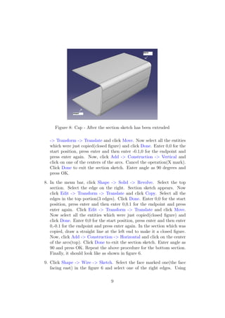
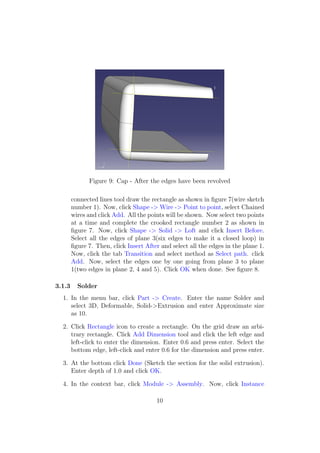
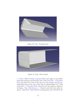
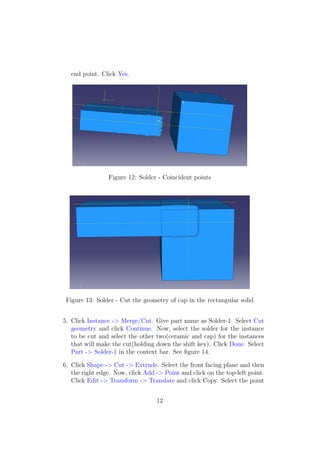
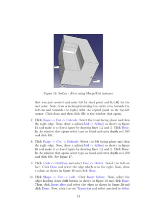
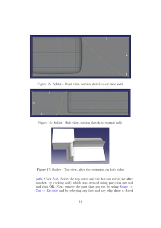
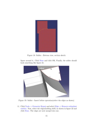
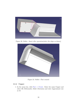
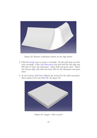
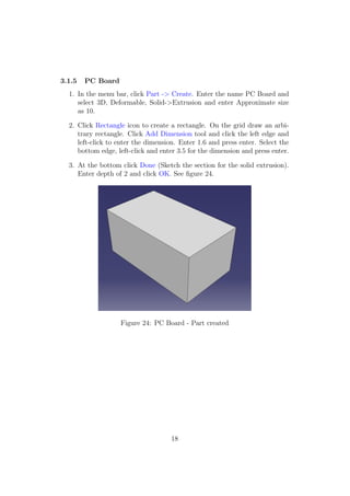
SlideShare a Scribd company logo
Finite-Element Project
  ABAQUS Tutorial
    Mohith Manjunath
      July 30, 2009


            1
Contents
1 Introduction                                                                                                            3

2 Problem Description                                                                                                     3

3 Pre-processing                                                                                                           4
  3.1 Part . . . . . . . . . .    .   .   .   .   .   .   .   .   .   .   .   .   .   .   .   .   .   .   .   .   .   .    5
      3.1.1 Ceramic . . . .       .   .   .   .   .   .   .   .   .   .   .   .   .   .   .   .   .   .   .   .   .   .    5
      3.1.2 Cap . . . . . .       .   .   .   .   .   .   .   .   .   .   .   .   .   .   .   .   .   .   .   .   .   .    6
      3.1.3 Solder . . . . .      .   .   .   .   .   .   .   .   .   .   .   .   .   .   .   .   .   .   .   .   .   .   10
      3.1.4 Copper . . . . .      .   .   .   .   .   .   .   .   .   .   .   .   .   .   .   .   .   .   .   .   .   .   16
      3.1.5 PC Board . . .        .   .   .   .   .   .   .   .   .   .   .   .   .   .   .   .   .   .   .   .   .   .   18
  3.2 Property . . . . . . . .    .   .   .   .   .   .   .   .   .   .   .   .   .   .   .   .   .   .   .   .   .   .   19
      3.2.1 Assign Sections       .   .   .   .   .   .   .   .   .   .   .   .   .   .   .   .   .   .   .   .   .   .   20
  3.3 Assembly . . . . . . .      .   .   .   .   .   .   .   .   .   .   .   .   .   .   .   .   .   .   .   .   .   .   21
  3.4 Step . . . . . . . . . .    .   .   .   .   .   .   .   .   .   .   .   .   .   .   .   .   .   .   .   .   .   .   22
  3.5 Interaction . . . . . . .   .   .   .   .   .   .   .   .   .   .   .   .   .   .   .   .   .   .   .   .   .   .   24
  3.6 Load . . . . . . . . . .    .   .   .   .   .   .   .   .   .   .   .   .   .   .   .   .   .   .   .   .   .   .   24
  3.7 Mesh . . . . . . . . . .    .   .   .   .   .   .   .   .   .   .   .   .   .   .   .   .   .   .   .   .   .   .   26
      3.7.1 Partitioning . .      .   .   .   .   .   .   .   .   .   .   .   .   .   .   .   .   .   .   .   .   .   .   26
      3.7.2 Meshing . . . .       .   .   .   .   .   .   .   .   .   .   .   .   .   .   .   .   .   .   .   .   .   .   37
  3.8 Job . . . . . . . . . . .   .   .   .   .   .   .   .   .   .   .   .   .   .   .   .   .   .   .   .   .   .   .   44

4 Postprocessing                                                          45
  4.1 Visualization . . . . . . . . . . . . . . . . . . . . . . . . . . . 45
      4.1.1 Selecting the field output to display . . . . . . . . . . . 45
      4.1.2 Plotting . . . . . . . . . . . . . . . . . . . . . . . . . . 45


                                              2
1    Introduction
ABAQUS is a finite-element analysis software. Abaqus/CAE provides a pre-
processing and postprocessing environment for the analysis of models. It is
used in a wide range of industries like automotive, aerospace etc., and also is
extensively used in academic and research institutions due to its capability
to address non-linear problems. The Abaqus interface is shown in figure 1.


                         Figure 1: Abaqus Interface

Get familiar with the icons in the tool bar especially the zoom icons which
are absolutely necessary in the modeling process.


2    Problem Description
Lifetime equations for micro-electronic solder needs to be predicted in order
to guarantee reliable in-field operation of micro-electronic components. Typ-
ical micro-electronic solder is shown in figure 2. The solder joints are under
thermo-mechanical stress due to the change in temperature during in-field
operation. Basically, there is a mismatch in coefficient of thermal expansion
between boards and components. This might lead to thermal fatigue failures

                                      3
and can be very catastrophic. Figure 3 shows the failure of solder joint after
many cycles in operation.


                       Figure 2: Microelectronic Solder


       Figure 3: Microelectronic Solder after 3000 cycles of operation


3     Pre-processing
Pre-processing is the initial phase of a finite element analysis program. This
phase includes various modules for creating a model, defining material prop-
erties, specifying boundary conditions and external loads and meshing the
assembly of the model.

    1. Start Abaqus CAE.

    2. Click Create Model Database to create a new model.

    3. The previous chapter explains the different sections of Abaqus.

    4. Continue with the next section for creating various parts of the model.

                                       4
3.1     Part
Part module is used to build different parts of the model. So, for convenience,
divide the whole model into various parts and create each part using this
module. Later all the parts can be assembled to form the entire model.
Here, the model is divided into five parts - Ceramic, Cap, Solder, Copper
and PC Board. What follows now is a step-by-step procedure to create each
of these parts.

3.1.1   Ceramic
  1. In the menu bar, click Part -> Create. Enter the name Ceramic and
     select 3D, Deformable, Solid->Extrusion and enter Approximate size
     as 10 (See Figure 4).


                       Figure 4: Create Ceramic Part

  2. Click Rectangle icon to create a rectangle. On the grid draw an arbi-
     trary rectangle. Click Add Dimension tool and click the left side and

                                      5
left-click to enter the dimension. Enter 0.25 and press enter. Select
        the bottom side, left-click and enter 1.0 for the dimension and press
        enter. Cancel procedure by pressing the ”X” mark in the ”prompt
        area”(remember to do this every time you want to come out of a pro-
        cedure and you can also press Esc key to exit an operation).

  3. At the bottom click Done (Sketch the section for the solid extrusion).
     Enter depth of 0.625 and click OK.

  4. From the menu bar, click Shape -> Blend -> Round/Fillet. Select
     the five edges as shown in Figure 5(Multiple edges can be selected by
     holding shift key). Click Done. Enter radius of 0.03. Click Done.


                Figure 5: For ceramic - Select the edges as shown


3.1.2     Cap
  1. In the menu bar, click Part -> Create. Enter the name Cap and select
     3D, Deformable, Solid->Extrusion and enter Approximate size as 10.

  2. Click Rectangle icon to create a rectangle. On the grid draw an arbi-
     trary rectangle. Click Add Dimension tool and click the left side and
     left-click to enter the dimension. Enter 0.25 and press enter. Select the
     bottom side, left-click and enter 0.3 for the dimension and press enter.

                                       6
3. In the menu bar, click Add -> Fillet. Enter fillet radius as 0.03 and
   press enter. Now, select the top and right side edges of the rectangle.
   Fillet has been created.

4. Click Add -> Point and create three points, one on the top left corner
   of the rectangle and two on the corners of the arc of the fillet(See Figure
   6). Click Edit -> Transform -> Translate and click Copy. Now, select
   the points 1 and 2(holding shift key) and click Done. Enter 0,0 for the
   start position, press enter and then enter 0,0.005 for the endpoint and
   press enter again. Repeat the same procedure for point 3 and enter
   0.005,0 for the endpoint. Repeat the same procedure for point 1 and
   enter 0.135,0.01 for the endpoint. Repeat the same procedure for point
   3 and enter 0,-0.095 for the endpoint. Repeat the same procedure for
   point 3 and enter 0.01,-0.095 for the endpoint.


        Figure 6: Section sketch for cap - Three points created


5. See Figure 7. Connect points 1 and 4 using Add -> Line -> Connected
   Lines. Also, draw a line through points 8 and 9 as shown in the figure.
   Suppose, while performing any of these operations if a point vanishes
   then you have to undo and zoom in to the area and complete the
   operation(keep this in mind). Now, click Add -> Spline and draw a
   spline through the points 4, 5 and 6(you might have to zoom in a bit).
   Repeat the same procedure for the points 7 and 8(first click point 7
   then click somewhere in the middle(as shown) and then click point 8).
   Now click Add -> Arc -> Center/Endpoints. Select the center of the
   circle(for the arc) and then select the two endpoints of the arc.

                                    7
Figure 7: Create spline through the points 4-5-6 and 7-8

6. Click Edit -> Split, select the right edge of the rectangle and then the
   horizontal line passing through the center of it. Now, click Edit ->
   Delete and select the left edge, bottom edge and the bottom half of the
   right edge(hold shift while selecting all three). Click Done. Now, click
   Edit -> Transform -> Mirror and click Copy. Then, pick the center
   horizontal line as the mirror line. Now select all the entities above the
   mirror line. Click Done. A mirror image is created. Now delete the
   center horizontal line. Click Done to exit the section sketch. Enter
   0.595 for depth and press OK.

7. In the menu bar, click Shape -> Solid -> Revolve. Select the plane
   section(C-Section) at the back(see figure 8) of the cap. Select one of
   the edges in the middle portion(vertical line in the C-Section). Section
   sketch appears(inverted C). Now click Edit -> Transform -> Translate
   and click Copy. Select all the edges in the middle portion and also
   the arcs at the top and bottom. Click Done. Enter 0,0 for the start
   position, press enter and then enter 0.1,0 for the endpoint and press
   enter again. In the section which was copied to the right, draw straight
   lines at top and bottom ends to make it a closed figure. Click Edit

                                   8
Figure 8: Cap - After the section sketch has been extruded

  -> Transform -> Translate and click Move. Now select all the entities
  which were just copied(closed figure) and click Done. Enter 0,0 for the
  start position, press enter and then enter -0.1,0 for the endpoint and
  press enter again. Now, click Add -> Construction -> Vertical and
  click on one of the centers of the arcs. Cancel the operation(X mark).
  Click Done to exit the section sketch. Enter angle as 90 degrees and
  press OK.

8. In the menu bar, click Shape -> Solid -> Revolve. Select the top
   section. Select the edge on the right. Section sketch appears. Now
   click Edit -> Transform -> Translate and click Copy. Select all the
   edges in the top portion(3 edges). Click Done. Enter 0,0 for the start
   position, press enter and then enter 0,0.1 for the endpoint and press
   enter again. Click Edit -> Transform -> Translate and click Move.
   Now select all the entities which were just copied(closed figure) and
   click Done. Enter 0,0 for the start position, press enter and then enter
   0,-0.1 for the endpoint and press enter again. In the section which was
   copied, draw a straight line at the left end to make it a closed figure.
   Now, click Add -> Construction -> Horizontal and click on the center
   of the arcs(top). Click Done to exit the section sketch. Enter angle as
   90 and press OK. Repeat the above procedure for the bottom section.
   Finally, it should look like as shown in figure 6.

9. Click Shape -> Wire -> Sketch. Select the face marked one(the face
   facing east) in the figure 6 and select one of the right edges. Using

                                   9
Figure 9: Cap - After the edges have been revolved

        connected lines tool draw the rectangle as shown in figure 7(wire sketch
        number 1). Now, click Shape -> Wire -> Point to point, select Chained
        wires and click Add. All the points will be shown. Now select two points
        at a time and complete the crooked rectangle number 2 as shown in
        figure 7. Now, click Shape -> Solid -> Loft and click Insert Before.
        Select all the edges of plane 3(six edges to make it a closed loop) in
        figure 7. Then, click Insert After and select all the edges in the plane 1.
        Now, click the tab Transition and select method as Select path. click
        Add. Now, select the edges one by one going from plane 3 to plane
        1(two edges in plane 2, 4 and 5). Click OK when done. See figure 8.

3.1.3     Solder
  1. In the menu bar, click Part -> Create. Enter the name Solder and
     select 3D, Deformable, Solid->Extrusion and enter Approximate size
     as 10.

  2. Click Rectangle icon to create a rectangle. On the grid draw an arbi-
     trary rectangle. Click Add Dimension tool and click the left edge and
     left-click to enter the dimension. Enter 0.6 and press enter. Select the
     bottom edge, left-click and enter 0.6 for the dimension and press enter.

  3. At the bottom click Done (Sketch the section for the solid extrusion).
     Enter depth of 1.0 and click OK.

  4. In the context bar, click Module -> Assembly. Now, click Instance

                                        10
Figure 10: Cap - Creating wires


                 Figure 11: Cap - Part created

-> Create. Select Ceramic, Cap and Solder and toggle on auto-offset
from other instances and click OK. Now, click Constraint -> Coincident
Point and select the center of the top arc in the ceramic and the cor-
responding point in the cap so that they fit together(figure 12). Click
Constraint -> Coincident Point and select the two points as shown in
the figure. Now, click Instance -> Translate and select the solder in-
stance. Click Done. Enter 0,0,0 for starting point and -0.27,0,0 for the


                               11
end point. Click Yes.


                Figure 12: Solder - Coincident points


 Figure 13: Solder - Cut the geometry of cap in the rectangular solid


5. Click Instance -> Merge/Cut. Give part name as Solder-1. Select Cut
   geometry and click Continue. Now, select the solder for the instance
   to be cut and select the other two(ceramic and cap) for the instances
   that will make the cut(holding down the shift key). Click Done. Select
   Part -> Solder-1 in the context bar. See figure 14.

6. Click Shape -> Cut -> Extrude. Select the front facing plane and then
   the right edge. Now, click Add -> Point and click on the top-left point.
   Click Edit -> Transform -> Translate and click Copy. Select the point


                                  12
Figure 14: Solder - After using Merge/Cut instance

    that was just created and enter 0,0 for start point and 0,-0.02 for the
    end point. Now, draw a rectangle(covering the entire area towards the
    bottom and towards the right) with the copied point as its top-left
    corner. Click done and then click OK in the window that opens.

 7. Click Shape -> Cut -> Extrude. Select the front facing plane and then
    the right edge. Now, draw a spline(Add -> Spline) as shown in figure
    15 and make it a closed figure by drawing lines 1,2 and 3. Click Done.
    In the window that opens select type as blind and enter depth as 0.595
    and click OK.

 8. Click Shape -> Cut -> Extrude. Select the left facing plane and then
    the right edge. Now, draw a spline(Add -> Spline) as shown in figure
    16 and make it a closed figure by drawing lines 1,2 and 3. Click Done.
    In the window that opens select type as blind and enter depth as 0.270
    and click OK. See figure 17.

 9. Click Tools -> Partition and select Face -> Sketch. Select the bottom
    face. Click Done and select the edge which is on the right. Now, draw
    a spline as shown in figure 18 and click Done.

10. Click Shape -> Cut -> Loft. Click Insert before. Now, select the
    edges holding down shift button as shown in figure 19 and click Done.
    Then, click Insert after and select the edges as shown in figure 20 and
    click Done. Now, click the tab Transition and select method as Select

                                   13
Figure 15: Solder - Front view, section sketch to extrude solid


 Figure 16: Solder - Side view, section sketch to extrude solid


Figure 17: Solder - Top view, after the extrusion on both sides

path. Click Add. Select the top curve and the bottom curve(one after
another, by clicking add) which was created using partition method
and click OK. Now, remove the part that got cut by using Shape ->
Cut -> Extrude and by selecting any face and any edge draw a closed


                               14
Figure 18: Solder - Bottom view, section sketch

    figure around it. Click Done and click OK. Finally, the solder should
    look something like figure 21.


 Figure 19: Solder - Insert before operation(select the edges as shown)


11. Click Tools -> Geometry Repair and select Edge -> Remove redundant
    entities. Now, select the edges(holding shift) as shown in figure 22 and
    click Done. The edges are now merged into one.

                                   15
Figure 20: Solder - Insert after operation(select the edges as shown)


                     Figure 21: Solder - Part created

3.1.4   Copper
  1. In the menu bar, click Part -> Create. Enter the name Copper and
     select 3D, Deformable, Solid->Extrusion and enter Approximate size
     as 10.


                                    16
Figure 22: Remove redundant entities on the edge shown

2. Click Rectangle icon to create a rectangle. On the grid draw an arbi-
   trary rectangle. Click Add Dimension tool and click the left edge and
   left-click to enter the dimension. Enter 0.06 and press enter. Select
   the bottom edge, left-click and enter 0.63 for the dimension and press
   enter.

3. At the bottom click Done (Sketch the section for the solid extrusion).
   Enter depth of 0.8 and click OK. See figure 23.


                  Figure 23: Copper - Part created


                                 17
3.1.5   PC Board
  1. In the menu bar, click Part -> Create. Enter the name PC Board and
     select 3D, Deformable, Solid->Extrusion and enter Approximate size
     as 10.

  2. Click Rectangle icon to create a rectangle. On the grid draw an arbi-
     trary rectangle. Click Add Dimension tool and click the left edge and
     left-click to enter the dimension. Enter 1.6 and press enter. Select the
     bottom edge, left-click and enter 3.5 for the dimension and press enter.

  3. At the bottom click Done (Sketch the section for the solid extrusion).
     Enter depth of 2 and click OK. See figure 24.


                   Figure 24: PC Board - Part created


                                    18
3.2    Property
Property module is used to define properties of various materials used in the
model. Then, sections are created and materials are assigned to each section.
This section of creating the properties of materials can be done later also, if
required to do so.
  1. In the context bar click Module -> Property to enter into property
     module.
  2. In the menu bar, click Material -> Manager.
  3. A new window opens. Now click the button Create to create new
     material.
  4. Enter the material name Ceramic and click Mechanical -> Elasticity
     -> Elastic. Now, enter the value 220000 MPa in the box below Young’s
     Modulus and 0.3 for Poisson’s Ratio. Click Mechanical -> Expansion
     and enter 8E-6 for Expansion Coeff alpha. Click OK.
  5. Click Create. Enter the material name Cap and click Mechanical -
     > Elasticity -> Elastic. Now, enter the value 120000 MPa in the box
     below Young’s Modulus and 0.31 for Poisson’s Ratio. Click Mechanical
     -> Expansion and enter 1.6E-5 for Expansion Coeff alpha. Click OK.
  6. Click Create. Enter the material name Solder-SnAgCu and click Me-
     chanical -> Elasticity -> Elastic. Now, enter the value 35000 MPa in
     the box below Young’s Modulus and 0.34 for Poisson’s Ratio. Click
     Mechanical -> Expansion and enter 2.3E-5 for Expansion Coeff alpha.
     Click Mechanical -> Plasticity -> Creep. In the drop-down menu for
     Law select Hyperbolic-Sine and enter the values shown in the table
     below. Hyperbolic-sine law is given by:
                                                −Q
                                             n
                               ε = C sinh(aσ )e RT
                               ˙                                           (1)
      Where ε is the strain rate, C is the power law multiplier, a the hyper-
              ˙
      bolic law multiplier, n the stress order, Q the activation energy and R
      the universal gas constant. The values of these parameters have been
      taken from reference 2.


        Power Law      Hyperb Law      Eq Stress           Activation    Universal Gas
       Multiplier(/s) Multiplier(/MPa)  Order           Energy(J/mol/K) Const(J/mol/K)
          4.41E5            0.005         4.2                4.5E4           8.314

                                      19
Click OK.

  7. Click Create. Enter the material name Copper and click Mechanical
     -> Elasticity -> Elastic. Now, enter the value 90000 MPa in the box
     below Young’s Modulus and 0.32 for Poisson’s Ratio. Click Mechanical
     -> Expansion and enter 1.65E-5 for Expansion Coeff alpha. Click OK.

  8. Click Create. Enter the material name FR4-PC Board and click Me-
     chanical -> Elasticity -> Elastic. In the drop-down menu for Type se-
     lect Engineering Constants and tick the checkbox next to Use temperature-
     dependent data and enter the following values. Directions 1,2 and 3
     refer to the X, Y and Z directions respectively in the material. The
     values have been taken from reference 3.

              E1(MPa) E2(MPa) E3(MPa) Nu12 Nu13 Nu23
               19300     8300      19300    0.4 0.15   0.4
                 G12(MPa) G13(MPa) G23(MPa) Temp(K)
                   8400       8400       8400      293

        Click Mechanical -> Expansion and select Type as Orthotropic and
        enter the following values.

                            alpha11 alpha22 alpha33
                             1.5E-5  8.4E-5  1.5E-5

        Click OK.

3.2.1     Assign Sections
After the materials have been creates we need to assign these materials to
the parts which were previously created.
  1. Click Section -> Create. Enter name as Ceramic. Select Solid ->
     Homogenous and click Continue. From the material list select Ceramic
     and click OK.

  2. Click Section -> Create. Enter name as Cap. Select Solid -> Homoge-
     nous and click Continue. From the material list select Cap and click
     OK.

  3. Click Section -> Create. Enter name as Solder. Select Solid -> Ho-
     mogenous and click Continue. From the material list select Solder-
     SnAgCu and click OK.

                                    20
4. Click Section -> Create. Enter name as Copper. Select Solid -> Ho-
     mogenous and click Continue. From the material list select Copper and
     click OK.
  5. Click Section -> Create. Enter name as PC Board. Select Solid ->
     Homogenous and click Continue. From the material list select FR4-PC
     Board and click OK.
  6. In the context bar select part as Ceramic. Click Assign -> Section.
     Select the ceramic by clicking on it and click Done. In the window that
     opens, select Ceramic from the list and click OK.
  7. In the context bar select part as Cap. Click Assign -> Section. Select
     the cap by clicking on it and click Done. In the window that opens,
     select Cap from the list and click OK.
  8. In the context bar select part as Solder-1. Click Assign -> Section.
     Select the solder by clicking on it and click Done. In the window that
     opens, select Solder from the list and click OK.
  9. In the context bar select part as Copper. Click Assign -> Section.
     Select the copper by clicking on it and click Done. In the window that
     opens, select Copper from the list and click OK.
 10. In the context bar select part as PC Board. Click Assign -> Section.
     Select the PC Board by clicking on it and click Done. In the window
     that opens, select PC Board from the list and click OK.
Now, the sections have been assigned to the parts with corresponding mate-
rial.

3.3    Assembly
In this module, all the parts created earlier can be put together(assembly)
to get the required model. After doing this we can apply the necessary
constraints and loads on the assembly.
  1. Select Module -> Assembly. Click Instance -> Create. Select Ceramic
     and Cap holding down Ctrl. Now, click Constraint -> Coincident point
     and select the center of the top arc in the ceramic and the corresponding
     point in the cap so that they fit together.
  2. Click Instance -> Create, select Solder-1 and toggle on auto-offset from
     other instances. Repeat the same procedure as before to make the
     solder fit right under the cap. See figure 21.

                                     21
Figure 25: Three instances assembled

  3. Click Instance -> Create, select Copper and toggle on auto-offset from
     other instances. Now, click Constraint -> Coincident point and select
     the top-left corner of copper and bottom-left corner of solder.

  4. Click Instance -> Create, select PC Board and toggle on auto-offset
     from other instances. Now, click Constraint -> Coincident point and
     select the top-left corner of PC Board and bottom-left corner of copper.
     Then, click Instance -> Translate and select PC Board instance. Enter
     0,0,0 for the start point and -0.7,0,0 for the end point and click yes and
     then OK. Now, all the instances have been assembled and take a look
     at the assembled model by rotating the figure. See figure 26.

  5. Click Instance -> Merge/Cut. Enter part name as Full-Model, select
     Merge -> Geometry and select Retain in intersecting boundaries section
     and click Continue. Now, select all the instances and click Done. All
     the instances are now merged and a new part by name Full-Model has
     been created.

3.4    Step
This module is used to perform many tasks, mainly to create analysis steps
and specify output requests.

  1. Select Module -> Step. Click Step -> Create. Type Extra-Step for
     name and select Procedure type -> General -> Visco and click Con-
     tinue. In the description field enter Abkhlung and enter time period as
     30. Go to incrementation tab and enter the following. Type:Automatic,


                                     22
Figure 26: All instances(Ceramic, Cap and Solder) assembled

  Maximum number of increments:10000, Increment size:Initial=0.5, Min=1E-
  6, Max=30, Tolerance=0.005 and Integration:Explicit/Implicit. Go to
  Other tab and select Iterative method and select ramp linearly over
  step. Click OK.

2. Select Module -> Step. Click Step -> Create. Type Step-1-Abkhlung
   for name and select Procedure type -> General -> Visco and click Con-
   tinue. Enter time period as 10. Go to incrementation tab and enter the
   following. Type:Automatic, Maximum number of increments:10000,
   Increment size:Initial=0.5, Min=1E-6, Max=10, Tolerance=0.005 and
   Integration:Explicit/Implicit. Go to Other tab and select Iterative
   method and select ramp linearly over step. Click OK.

3. Select Module -> Step. Click Step -> Create. Type Step-2-Halten-
   40C for name and select Procedure type -> General -> Visco and
   click Continue. Enter time period as 900. Go to incrementation tab
   and enter the following. Type:Automatic, Maximum number of incre-
   ments:10000, Increment size:Initial=0.5, Min=1E-6, Max=900, Toler-
   ance=0.005 and Integration:Explicit/Implicit. Go to Other tab and
   select Iterative method and select ramp linearly over step. Click OK.


                                 23
4. Select Module -> Step. Click Step -> Create. Type Step-3-Aufheizen
     for name and select Procedure type -> General -> Visco and click Con-
     tinue. Enter time period as 10. Go to incrementation tab and enter the
     following. Type:Automatic, Maximum number of increments:10000,
     Increment size:Initial=0.5, Min=1E-6, Max=10, Tolerance=0.005 and
     Integration:Explicit/Implicit. Go to Other tab and select Iterative
     method and select ramp linearly over step. Click OK.

  5. Select Module -> Step. Click Step -> Create. Type Step-4-Halten-
     auf-125C for name and select Procedure type -> General -> Visco and
     click Continue. Enter time period as 900. Go to incrementation tab
     and enter the following. Type:Automatic, Maximum number of incre-
     ments:10000, Increment size:Initial=0.5, Min=1E-6, Max=900, Toler-
     ance=0.005 and Integration:Explicit/Implicit. Go to Other tab and
     select Iterative method and select ramp linearly over step. Click OK.

3.5    Interaction
As the name suggests, this module is used to define various interactions
within the model or interactions between regions of the model and its sur-
roundings. The interactions can be mechanical or/and thermal. Analysis
constraints can also be applied between regions of the model.

3.6    Load
Load module is used to define and manage various conditions like loads,
boundary conditions and predefined fields.

  1. Select Module -> Load. Click BC -> Create. Select Displacement/Rotation
     and click Continue. Select the whole of left section(plane) and hold
     down control key to deselect the bottom-left point(see figure 27). Click
     Done and then just tick the box next to U1 to constrain that degree of
     freedom.

  2. Click BC -> Create. Select Displacement/Rotation and click Continue.
     Select the corner point which was previously not selected and click
     Done and then just tick the box next to U2 to constrain that degree of
     freedom.

  3. Click BC -> Create. Select Displacement/Rotation and click Continue.
     Select the whole of front section(plane X-Y)(for easier selection click
     the icon in the ”prompt area” and select faces from the list and then

                                    24
Figure 27: Boundary Condition on the left face - U1 constrained

  select ”by angle” from the list in the prompt area) and click Done and
  then just tick the box next to U3 to constrain that degree of freedom.


 Figure 28: Boundary Condition on the front face - U3 constrained


4. Click Predefined Field -> Create. Select Other -> Temperature and
   click Continue. Select the whole assembly and click Done and then
   enter 421 for the magnitude of temperature. Click OK.


                                 25
Figure 29: Predefined Field - Initial temperature for the entire model

3.7     Mesh
This is one of the most important modules since accuracy of the results
will depend on the meshing of the assemblies. This module can be used to
generate meshes and even verify them.

3.7.1   Partitioning
  1. Select Part -> Full-Model from the list in the left window. Select
     Module -> Mesh. See figure 30.

  2. Click Tools -> Partition. Select Cell -> Extend face, select the entire
     model and click Done. Select the face as shown in the figure 31 and
     click Create partition. A partition should be created and it should
     turn green(structured mesh). Repeat the same procedure for the faces
     as shown in the figure 32 and 33 and now entire PC Board should turn
     green(figure 33).

  3. Select Cell -> Extrude/Sweep edges, select the entire model and the
     edge 1(choose by edge angle) as shown in figure 34. Click Done. Select
     Extrude Along Direction and select the edge 2(pointing down) as shown
     in the same figure. Check for direction and flip if required. Click Create
     partition. See figure 35.


                                    26
Figure 30: Partitions are required for the whole model(for orange colored
ones, it is mandatory)


                    Figure 31: Partition - Extend face


                                   27
Figure 32: Partition - Extend face


Figure 33: Partition - Extend face


               28
Figure 34: Partition - Extrude edges


                29
Figure 35: Partition - The edges have been extruded


                        30
4. Select Cell -> Define cutting plane, select the entire model and click
     Done. Then, click Point and Normal. And select point and normal as
     shown in the figure 36 and click Create partition. See figure 37.


Figure 36: Partition - Select the point as pointed by the arrow and the line
in pink


  5. Select Cell -> Define cutting plane, select the entire model and click
     Done. Then, click Point and Normal. And select point and normal as
     shown in the figure 38 and click Create partition. See figure 39.

  6. Select Cell -> Define cutting plane, select the entire model and click
     Done. Then, click Point and Normal. And select point and normal as
     shown in the figure 40 and click Create partition. At the end of this
     operation, the model should look similar to figure 41.


                                    31
Figure 37: Partition - At the end of previous operation


                          32
Figure 38: Partition - Select the point as pointed by the arrow and the line
in pink


          Figure 39: Partition - At the end of previous operation


                                    33
Figure 40: Partition - Select the point as pointed by the arrow and the line
in pink


          Figure 41: Partition - At the end of previous operation


                                    34
7. Select Cell -> Define cutting plane, select the entire model and click
     Done. Then, click Point and Normal. And select point and normal as
     shown in the figure 42 and click Create partition. At the end of this
     operation, the model should look similar to figure 43.


Figure 42: Partition - Select the point as pointed by the arrow and the line
in pink


          Figure 43: Partition - At the end of previous operation


                                    35
8. Select Cell -> Define cutting plane, select the entire model and click
     Done. Then, click Point and Normal. And select point and normal as
     shown in the figure 44 and click Create partition. At the end of this
     operation, the model should look similar to figure 45.


Figure 44: Partition - Select the point as pointed by the arrow and the line
in pink


            Figure 45: Partitioning done - Everything is green!


                                    36
Now, you can proceed to the meshing section but it is suggested that you
try different partitioning methods and analyze the results. In the process
you will be able to learn how to partition any complicated geometry with
minimum partitioning.

3.7.2   Meshing
  1. Click Mesh -> Controls. Select the entire model, click Done and select
     Structured from the list and click OK.

  2. Click Mesh -> Element Type. Select the entire model, accept the
     default options and click OK.

  3. Click Seed -> Part. In the approximate global size field enter 0.01 and
     click OK.

  4. Click Seed -> Edge Biased. Switch to wire-frame view. Select the
     edges(click near the left end of the edges) as shown in the figure 46 and
     click Done. Enter bias ratio as 10 and number of elements as 18.


             Figure 46: Edges biased towards the solder(left)


  5. Click Seed -> Edge Biased. Select the edges(click near the top end of
     the edges) as shown in the figure 47 and click Done. Enter bias ratio
     as 10 and number of elements as 18.


                                    37
Figure 47: Edges biased towards the solder(top)


                      38
6. Click Seed -> Edge Biased. Select the edges(click near the right end of
   the edges) as shown in the figure 48 and click Done. Enter bias ratio
   as 10 and number of elements as 8.


          Figure 48: Edges biased towards the solder(right)


7. Click Seed -> Edge Biased. Select the edges(click near the bottom end
   of the edges) as shown in the figure 49 and click Done. Enter bias ratio
   as 10 and number of elements as 16.


        Figure 49: Edges biased(Top view) towards the solder


                                  39
8. Click Seed -> Edge Biased. Select the edges(click near the top end of
    the edges) as shown in the figure 50 and click Done. Enter bias ratio
    as 10 and number of elements as 8.


         Figure 50: Edges biased(Top view) towards the solder


 9. Now, click the create display group icon, select ceramic from the list
    of sets and click replace. Click Seed -> Edge By Number. Select the
    edges as shown in the figure 51 and enter 14 for the number of elements.


Figure 51: Ceramic - ”Edge by number” operation for the edges shown


10. Click Mesh -> Controls and select all the cells except the ones in the
    corner edge(see figure 52). Click Done and in the window that opens
    select Sweep and click OK. Then, click Mesh -> Region and select all
    the cells(the whole ceramic) and click Done. See figure 53.

                                   40
Figure 52: Ceramic - Select all except the cells in green


                        Figure 53: Ceramic Mesh

11. Now, click the create display group icon, select cap from the list of sets
    and click replace. Click Mesh -> Region and select all the cells and
    click OK.


                                    41
12. Now, click the create display group icon, select solder from the list of
    sets and click replace. Click Seed -> Edge By Number. Select the edges
    as shown in the figure 54 and enter 14 for the number of elements.


 Figure 54: Solder - ”Edge by number” operation for the edges shown


13. Click Mesh -> Controls and select all the cells except the ones in the
    corner edge(see figure 55). Click Done and in the window that opens
    select Sweep and click OK. Then, click Mesh -> Region and select all
    the cells(the whole solder) and click Done. See figure 56.


              Figure 55: Solder - Select the cells as shown


                                   42
Figure 56: Solder Mesh

14. Now, click the create display group icon, select PC Board from the list
    of sets and click replace. Click Mesh -> Region and select all the cells
    and click OK.

15. Now, click the create display group icon, select copper from the list of
    sets and click replace. Click Mesh -> Controls and select all the cells.
    Click Done and in the window that opens select Sweep and click OK.
    Then, click Mesh -> Region and select all the cells and click OK.


                Figure 57: Complete Mesh of the model

                                   43
It should be noted that the mesh created above is not a perfect mesh.
      There are quite a few dark patches which should not have been there.
      I would suggest, since you have gained a little experience in Abaqus
      now, you to experiment with the mesh by playing around with the mesh
      controls, seeding etc., so that you will become familiar with different
      kinds of meshes. Then, you can try to create a better mesh than this
      one and be proud of doing it.

3.8    Job
Job module can be used to create and manage analysis jobs and submit them
for analysis.

  1. Select Module -> Job.

  2. Click Job -> Manager. In the window that opens, click Create. Enter
     job name as 3DSolder and click Continue. Now, just explore all the
     tabs and leave the default options as it is. Click OK. Now, select the
     current job and click Submit. After the job has been submitted, the
     analysis can be monitored by clicking Monitor.


                                     44
4       Postprocessing
The results generated from the analysis can be enormous so it requires ad-
ditional processing which is termed postprocessing.

4.1     Visualization
Here the model can be viewed and various plots can be generated.

4.1.1    Selecting the field output to display
    1. Select Result -> Field Output from the main menu bar. Here, one of
       the various parameters like CEEQ, PEEQ, stress components etc. can
       be selected. Click OK.

4.1.2    Plotting
    1. To plot undeformed shape select Plot -> Undeformed Shape from the
       main menu bar.

    2. To plot deformed shape select Plot -> Deformed Shape from the main
       menu bar.

Here, not all the modules of postprocessing are explained. You can explore
different modules and try to generate plots for different parameters and get
meaningful results out of them.


                                    45
Bibliography
 1. Abaqus 6.7-4 Documentation.

 2. Improving Solder Joint Reliability of WLP by Means of a Compliant
    Layer , Lee Hun Kwang et al., International Electronic Manufacturing
    Technology 2006

 3. FEM-Simulationen und Zuverlssigkeit von Advanced Packages LWF,
    Uni Paderborn, IFM, TU Berlin


                                  46

More Related Content

What's hot

Introduction to ANSYS Workbench
Introduction to ANSYS WorkbenchIntroduction to ANSYS Workbench
Introduction to ANSYS Workbench
nagesh surner
 
Abaqus modelling and_analysis
Abaqus modelling and_analysisAbaqus modelling and_analysis
Abaqus modelling and_analysis
Debanshu Sharma
 
Hướng dẫn sử dụng SACS 5.6
Hướng dẫn sử dụng SACS 5.6Hướng dẫn sử dụng SACS 5.6
Hướng dẫn sử dụng SACS 5.6luuguxd
 
ansys tutorial
ansys tutorialansys tutorial
ansys tutorial
Pradeep kumar
 
Fem ppt swapnil
Fem ppt swapnilFem ppt swapnil
Fem ppt swapnil
Nerusu Mangapathi
 
Solidworks ppt 2015
Solidworks ppt 2015Solidworks ppt 2015
Solidworks ppt 2015
lalit yadav
 
Finite Element Analysis - UNIT-2
Finite Element Analysis - UNIT-2Finite Element Analysis - UNIT-2
Finite Element Analysis - UNIT-2
propaul
 
5. stress function
5.  stress function5.  stress function
5. stress function
YASWANTH BHAIRAVABHOTLA
 
Theories of failure_scet
Theories of failure_scetTheories of failure_scet
Theories of failure_scet
Gagandeep singh
 
Finite Element Analysis - UNIT-3
Finite Element Analysis - UNIT-3Finite Element Analysis - UNIT-3
Finite Element Analysis - UNIT-3
propaul
 
Ansys beam problem
Ansys beam problemAnsys beam problem
Ansys beam problem
nmahi96
 
AUTOCAD Report
AUTOCAD ReportAUTOCAD Report
AUTOCAD Report
AMIT RAJ
 
Numerical modeling of concrete in Abaqus
Numerical modeling of concrete in Abaqus Numerical modeling of concrete in Abaqus
Numerical modeling of concrete in Abaqus
Harish Kant Soni
 
Buckling Analysis in ANSYS
Buckling Analysis in ANSYSBuckling Analysis in ANSYS
Buckling Analysis in ANSYS
Maha Hassan
 
Tutor abaqus 2.
Tutor abaqus 2.Tutor abaqus 2.
Tutor abaqus 2.
Alpian Saputra
 
Catia v5 NOTES
Catia v5  NOTESCatia v5  NOTES
Catia v5 NOTES
vipinshelke
 
Solidworks
SolidworksSolidworks
Solidworks
Pawan Kumar
 
Finite element method
Finite element methodFinite element method
Finite element method
MANISH RANJAN
 
Setting up a crash simulation in LS-Dyna
Setting up a crash simulation in LS-DynaSetting up a crash simulation in LS-Dyna
Setting up a crash simulation in LS-Dyna
Akshay Mistri
 

What's hot (20)

Introduction to ANSYS Workbench
Introduction to ANSYS WorkbenchIntroduction to ANSYS Workbench
Introduction to ANSYS Workbench
 
Abaqus modelling and_analysis
Abaqus modelling and_analysisAbaqus modelling and_analysis
Abaqus modelling and_analysis
 
Hướng dẫn sử dụng SACS 5.6
Hướng dẫn sử dụng SACS 5.6Hướng dẫn sử dụng SACS 5.6
Hướng dẫn sử dụng SACS 5.6
 
ansys tutorial
ansys tutorialansys tutorial
ansys tutorial
 
Fem ppt swapnil
Fem ppt swapnilFem ppt swapnil
Fem ppt swapnil
 
Solidworks ppt 2015
Solidworks ppt 2015Solidworks ppt 2015
Solidworks ppt 2015
 
Finite Element Analysis - UNIT-2
Finite Element Analysis - UNIT-2Finite Element Analysis - UNIT-2
Finite Element Analysis - UNIT-2
 
5. stress function
5.  stress function5.  stress function
5. stress function
 
Theories of failure_scet
Theories of failure_scetTheories of failure_scet
Theories of failure_scet
 
Finite Element Analysis - UNIT-3
Finite Element Analysis - UNIT-3Finite Element Analysis - UNIT-3
Finite Element Analysis - UNIT-3
 
Ansys beam problem
Ansys beam problemAnsys beam problem
Ansys beam problem
 
AUTOCAD Report
AUTOCAD ReportAUTOCAD Report
AUTOCAD Report
 
Hdsd sacs 5.2
Hdsd sacs 5.2Hdsd sacs 5.2
Hdsd sacs 5.2
 
Numerical modeling of concrete in Abaqus
Numerical modeling of concrete in Abaqus Numerical modeling of concrete in Abaqus
Numerical modeling of concrete in Abaqus
 
Buckling Analysis in ANSYS
Buckling Analysis in ANSYSBuckling Analysis in ANSYS
Buckling Analysis in ANSYS
 
Tutor abaqus 2.
Tutor abaqus 2.Tutor abaqus 2.
Tutor abaqus 2.
 
Catia v5 NOTES
Catia v5  NOTESCatia v5  NOTES
Catia v5 NOTES
 
Solidworks
SolidworksSolidworks
Solidworks
 
Finite element method
Finite element methodFinite element method
Finite element method
 
Setting up a crash simulation in LS-Dyna
Setting up a crash simulation in LS-DynaSetting up a crash simulation in LS-Dyna
Setting up a crash simulation in LS-Dyna
 

Viewers also liked

آموزش نرم افزار آنالیز اجزای محدود ABAQUS
آموزش نرم افزار آنالیز اجزای محدود ABAQUSآموزش نرم افزار آنالیز اجزای محدود ABAQUS
آموزش نرم افزار آنالیز اجزای محدود ABAQUS
faradars
 
ABAQUS Lecture Part II
ABAQUS Lecture Part IIABAQUS Lecture Part II
ABAQUS Lecture Part II
chimco.net
 
COMPUTATIONAL ENGINEERING OF FINITE ELEMENT MODELLING FOR AUTOMOTIVE APPLICAT...
COMPUTATIONAL ENGINEERING OF FINITE ELEMENT MODELLING FOR AUTOMOTIVE APPLICAT...COMPUTATIONAL ENGINEERING OF FINITE ELEMENT MODELLING FOR AUTOMOTIVE APPLICAT...
COMPUTATIONAL ENGINEERING OF FINITE ELEMENT MODELLING FOR AUTOMOTIVE APPLICAT...
IAEME Publication
 
1 1 abaqus tutorial
1 1 abaqus tutorial1 1 abaqus tutorial
1 1 abaqus tutorial
nghiahanh
 
1 2 learning abaqus
1 2 learning abaqus1 2 learning abaqus
1 2 learning abaqus
senthil kumar rsk
 
فرکانس طبیعی های حساب شده برای پنج مود اول تیر یک سر گیردار
فرکانس طبیعی های حساب شده برای  پنج مود اول تیر یک سر گیردار فرکانس طبیعی های حساب شده برای  پنج مود اول تیر یک سر گیردار
فرکانس طبیعی های حساب شده برای پنج مود اول تیر یک سر گیردار
maryam ghasemzadeh
 
Abaqus tutorial
Abaqus tutorialAbaqus tutorial
Abaqus tutorial
Deivids Hyggelig
 
FEA Final Project
FEA Final ProjectFEA Final Project
FEA Final Project
Benjamin Salisbury
 
Abaqusfracture mechanics
Abaqusfracture mechanicsAbaqusfracture mechanics
Abaqusfracture mechanics
imransuces
 
An Introduction to ABAQUS CAE
An Introduction to ABAQUS CAEAn Introduction to ABAQUS CAE
An Introduction to ABAQUS CAE
Fawad Najam
 
أقوى مذكرة حساب جبر للصف الثالث الابتدائي ترم أول 2015
أقوى مذكرة حساب جبر للصف الثالث الابتدائي ترم أول 2015أقوى مذكرة حساب جبر للصف الثالث الابتدائي ترم أول 2015
أقوى مذكرة حساب جبر للصف الثالث الابتدائي ترم أول 2015
أمنية وجدى
 

Viewers also liked (11)

آموزش نرم افزار آنالیز اجزای محدود ABAQUS
آموزش نرم افزار آنالیز اجزای محدود ABAQUSآموزش نرم افزار آنالیز اجزای محدود ABAQUS
آموزش نرم افزار آنالیز اجزای محدود ABAQUS
 
ABAQUS Lecture Part II
ABAQUS Lecture Part IIABAQUS Lecture Part II
ABAQUS Lecture Part II
 
COMPUTATIONAL ENGINEERING OF FINITE ELEMENT MODELLING FOR AUTOMOTIVE APPLICAT...
COMPUTATIONAL ENGINEERING OF FINITE ELEMENT MODELLING FOR AUTOMOTIVE APPLICAT...COMPUTATIONAL ENGINEERING OF FINITE ELEMENT MODELLING FOR AUTOMOTIVE APPLICAT...
COMPUTATIONAL ENGINEERING OF FINITE ELEMENT MODELLING FOR AUTOMOTIVE APPLICAT...
 
1 1 abaqus tutorial
1 1 abaqus tutorial1 1 abaqus tutorial
1 1 abaqus tutorial
 
1 2 learning abaqus
1 2 learning abaqus1 2 learning abaqus
1 2 learning abaqus
 
فرکانس طبیعی های حساب شده برای پنج مود اول تیر یک سر گیردار
فرکانس طبیعی های حساب شده برای  پنج مود اول تیر یک سر گیردار فرکانس طبیعی های حساب شده برای  پنج مود اول تیر یک سر گیردار
فرکانس طبیعی های حساب شده برای پنج مود اول تیر یک سر گیردار
 
Abaqus tutorial
Abaqus tutorialAbaqus tutorial
Abaqus tutorial
 
FEA Final Project
FEA Final ProjectFEA Final Project
FEA Final Project
 
Abaqusfracture mechanics
Abaqusfracture mechanicsAbaqusfracture mechanics
Abaqusfracture mechanics
 
An Introduction to ABAQUS CAE
An Introduction to ABAQUS CAEAn Introduction to ABAQUS CAE
An Introduction to ABAQUS CAE
 
أقوى مذكرة حساب جبر للصف الثالث الابتدائي ترم أول 2015
أقوى مذكرة حساب جبر للصف الثالث الابتدائي ترم أول 2015أقوى مذكرة حساب جبر للصف الثالث الابتدائي ترم أول 2015
أقوى مذكرة حساب جبر للصف الثالث الابتدائي ترم أول 2015
 

Similar to Abaqus tutorial -_3_d_solder

Circuitikzmanual (1)
Circuitikzmanual (1)Circuitikzmanual (1)
Circuitikzmanual (1)
Geraldo Silva
 
finalproject1 finished
finalproject1 finishedfinalproject1 finished
finalproject1 finished
James Cianciolo
 
Master Thesis
Master ThesisMaster Thesis
Master Thesis
Navid Rahimi
 
Arcanoid 3D
Arcanoid 3DArcanoid 3D
Arcanoid 3D
graphitech
 
Learn c++
Learn c++Learn c++
Learn c++
aashay1996
 
How to make a good CAD file for induction heating simulation
How to make a good CAD file for induction heating simulationHow to make a good CAD file for induction heating simulation
How to make a good CAD file for induction heating simulation
Cenos LLC
 
Grafx
GrafxGrafx
A Report on Baseball Using R
A Report on Baseball Using RA Report on Baseball Using R
A Report on Baseball Using R
Raymond Christopher Peralta
 
Heat source simulation
Heat source simulationHeat source simulation
Heat source simulation
Braj Bhushan Prasad
 
User manual of feko
User manual of fekoUser manual of feko
User manual of feko
Jojo Namy
 
Coupled thermal fluid analysis with flowpath-cavity interaction in a gas turb...
Coupled thermal fluid analysis with flowpath-cavity interaction in a gas turb...Coupled thermal fluid analysis with flowpath-cavity interaction in a gas turb...
Coupled thermal fluid analysis with flowpath-cavity interaction in a gas turb...
Nathan Fitzpatrick
 
Reading Materials for Operational Research
Reading Materials for Operational Research Reading Materials for Operational Research
Reading Materials for Operational Research
Derbew Tesfa
 
ZW3D CAD/CAM Excise
ZW3D CAD/CAM ExciseZW3D CAD/CAM Excise
ZW3D CAD/CAM Excise
Wing Zhu
 
FDTD-FEM Hybrid
FDTD-FEM HybridFDTD-FEM Hybrid
FDTD-FEM Hybrid
kickaplan
 
Keypoints manual
Keypoints manualKeypoints manual
Keypoints manual
Khaled Ramadan
 
Final_report
Final_reportFinal_report
Final_report
Marko Tanaskovic
 
Mechanical Lifting machine | Design project | Mechanical Engineering Undergra...
Mechanical Lifting machine | Design project | Mechanical Engineering Undergra...Mechanical Lifting machine | Design project | Mechanical Engineering Undergra...
Mechanical Lifting machine | Design project | Mechanical Engineering Undergra...
PrasanthNadarajah1
 
Winning noble
Winning nobleWinning noble
Winning noble
stryfe10
 
2D ROBOTIC PLOTTER
2D ROBOTIC PLOTTER2D ROBOTIC PLOTTER
2D ROBOTIC PLOTTER
ANANDKRISHNANVSSS
 
Fabric Defect Detaction in Frequency Domain Using Fourier Analysis
Fabric Defect Detaction in Frequency Domain Using Fourier AnalysisFabric Defect Detaction in Frequency Domain Using Fourier Analysis
Fabric Defect Detaction in Frequency Domain Using Fourier Analysis
Gokay Titrek
 

Similar to Abaqus tutorial -_3_d_solder (20)

Circuitikzmanual (1)
Circuitikzmanual (1)Circuitikzmanual (1)
Circuitikzmanual (1)
 
finalproject1 finished
finalproject1 finishedfinalproject1 finished
finalproject1 finished
 
Master Thesis
Master ThesisMaster Thesis
Master Thesis
 
Arcanoid 3D
Arcanoid 3DArcanoid 3D
Arcanoid 3D
 
Learn c++
Learn c++Learn c++
Learn c++
 
How to make a good CAD file for induction heating simulation
How to make a good CAD file for induction heating simulationHow to make a good CAD file for induction heating simulation
How to make a good CAD file for induction heating simulation
 
Grafx
GrafxGrafx
Grafx
 
A Report on Baseball Using R
A Report on Baseball Using RA Report on Baseball Using R
A Report on Baseball Using R
 
Heat source simulation
Heat source simulationHeat source simulation
Heat source simulation
 
User manual of feko
User manual of fekoUser manual of feko
User manual of feko
 
Coupled thermal fluid analysis with flowpath-cavity interaction in a gas turb...
Coupled thermal fluid analysis with flowpath-cavity interaction in a gas turb...Coupled thermal fluid analysis with flowpath-cavity interaction in a gas turb...
Coupled thermal fluid analysis with flowpath-cavity interaction in a gas turb...
 
Reading Materials for Operational Research
Reading Materials for Operational Research Reading Materials for Operational Research
Reading Materials for Operational Research
 
ZW3D CAD/CAM Excise
ZW3D CAD/CAM ExciseZW3D CAD/CAM Excise
ZW3D CAD/CAM Excise
 
FDTD-FEM Hybrid
FDTD-FEM HybridFDTD-FEM Hybrid
FDTD-FEM Hybrid
 
Keypoints manual
Keypoints manualKeypoints manual
Keypoints manual
 
Final_report
Final_reportFinal_report
Final_report
 
Mechanical Lifting machine | Design project | Mechanical Engineering Undergra...
Mechanical Lifting machine | Design project | Mechanical Engineering Undergra...Mechanical Lifting machine | Design project | Mechanical Engineering Undergra...
Mechanical Lifting machine | Design project | Mechanical Engineering Undergra...
 
Winning noble
Winning nobleWinning noble
Winning noble
 
2D ROBOTIC PLOTTER
2D ROBOTIC PLOTTER2D ROBOTIC PLOTTER
2D ROBOTIC PLOTTER
 
Fabric Defect Detaction in Frequency Domain Using Fourier Analysis
Fabric Defect Detaction in Frequency Domain Using Fourier AnalysisFabric Defect Detaction in Frequency Domain Using Fourier Analysis
Fabric Defect Detaction in Frequency Domain Using Fourier Analysis
 

Recently uploaded

How to Get CNIC Information System with Paksim Ga.pptx
How to Get CNIC Information System with Paksim Ga.pptxHow to Get CNIC Information System with Paksim Ga.pptx
How to Get CNIC Information System with Paksim Ga.pptx
danishmna97
 
Best 20 SEO Techniques To Improve Website Visibility In SERP
Best 20 SEO Techniques To Improve Website Visibility In SERPBest 20 SEO Techniques To Improve Website Visibility In SERP
Best 20 SEO Techniques To Improve Website Visibility In SERP
Pixlogix Infotech
 
Communications Mining Series - Zero to Hero - Session 1
Communications Mining Series - Zero to Hero - Session 1Communications Mining Series - Zero to Hero - Session 1
Communications Mining Series - Zero to Hero - Session 1
DianaGray10
 
Mind map of terminologies used in context of Generative AI
Mind map of terminologies used in context of Generative AIMind map of terminologies used in context of Generative AI
Mind map of terminologies used in context of Generative AI
Kumud Singh
 
Video Streaming: Then, Now, and in the Future
Video Streaming: Then, Now, and in the FutureVideo Streaming: Then, Now, and in the Future
Video Streaming: Then, Now, and in the Future
Alpen-Adria-Universität
 
GraphSummit Singapore | The Art of the Possible with Graph - Q2 2024
GraphSummit Singapore | The Art of the  Possible with Graph - Q2 2024GraphSummit Singapore | The Art of the  Possible with Graph - Q2 2024
GraphSummit Singapore | The Art of the Possible with Graph - Q2 2024
Neo4j
 
Climate Impact of Software Testing at Nordic Testing Days
Climate Impact of Software Testing at Nordic Testing DaysClimate Impact of Software Testing at Nordic Testing Days
Climate Impact of Software Testing at Nordic Testing Days
Kari Kakkonen
 
20240607 QFM018 Elixir Reading List May 2024
20240607 QFM018 Elixir Reading List May 202420240607 QFM018 Elixir Reading List May 2024
20240607 QFM018 Elixir Reading List May 2024
Matthew Sinclair
 
Infrastructure Challenges in Scaling RAG with Custom AI models
Infrastructure Challenges in Scaling RAG with Custom AI modelsInfrastructure Challenges in Scaling RAG with Custom AI models
Infrastructure Challenges in Scaling RAG with Custom AI models
Zilliz
 
GenAI Pilot Implementation in the organizations
GenAI Pilot Implementation in the organizationsGenAI Pilot Implementation in the organizations
GenAI Pilot Implementation in the organizations
kumardaparthi1024
 
20240605 QFM017 Machine Intelligence Reading List May 2024
20240605 QFM017 Machine Intelligence Reading List May 202420240605 QFM017 Machine Intelligence Reading List May 2024
20240605 QFM017 Machine Intelligence Reading List May 2024
Matthew Sinclair
 
GraphSummit Singapore | The Future of Agility: Supercharging Digital Transfor...
GraphSummit Singapore | The Future of Agility: Supercharging Digital Transfor...GraphSummit Singapore | The Future of Agility: Supercharging Digital Transfor...
GraphSummit Singapore | The Future of Agility: Supercharging Digital Transfor...
Neo4j
 
Building Production Ready Search Pipelines with Spark and Milvus
Building Production Ready Search Pipelines with Spark and MilvusBuilding Production Ready Search Pipelines with Spark and Milvus
Building Production Ready Search Pipelines with Spark and Milvus
Zilliz
 
Uni Systems Copilot event_05062024_C.Vlachos.pdf
Uni Systems Copilot event_05062024_C.Vlachos.pdfUni Systems Copilot event_05062024_C.Vlachos.pdf
Uni Systems Copilot event_05062024_C.Vlachos.pdf
Uni Systems S.M.S.A.
 
Pushing the limits of ePRTC: 100ns holdover for 100 days
Pushing the limits of ePRTC: 100ns holdover for 100 daysPushing the limits of ePRTC: 100ns holdover for 100 days
Pushing the limits of ePRTC: 100ns holdover for 100 days
Adtran
 
HCL Notes und Domino Lizenzkostenreduzierung in der Welt von DLAU
HCL Notes und Domino Lizenzkostenreduzierung in der Welt von DLAUHCL Notes und Domino Lizenzkostenreduzierung in der Welt von DLAU
HCL Notes und Domino Lizenzkostenreduzierung in der Welt von DLAU
panagenda
 
Serial Arm Control in Real Time Presentation
Serial Arm Control in Real Time PresentationSerial Arm Control in Real Time Presentation
Serial Arm Control in Real Time Presentation
tolgahangng
 
UiPath Test Automation using UiPath Test Suite series, part 5
UiPath Test Automation using UiPath Test Suite series, part 5UiPath Test Automation using UiPath Test Suite series, part 5
UiPath Test Automation using UiPath Test Suite series, part 5
DianaGray10
 
GraphSummit Singapore | Graphing Success: Revolutionising Organisational Stru...
GraphSummit Singapore | Graphing Success: Revolutionising Organisational Stru...GraphSummit Singapore | Graphing Success: Revolutionising Organisational Stru...
GraphSummit Singapore | Graphing Success: Revolutionising Organisational Stru...
Neo4j
 
Driving Business Innovation: Latest Generative AI Advancements & Success Story
Driving Business Innovation: Latest Generative AI Advancements & Success StoryDriving Business Innovation: Latest Generative AI Advancements & Success Story
Driving Business Innovation: Latest Generative AI Advancements & Success Story
Safe Software
 

Recently uploaded (20)

How to Get CNIC Information System with Paksim Ga.pptx
How to Get CNIC Information System with Paksim Ga.pptxHow to Get CNIC Information System with Paksim Ga.pptx
How to Get CNIC Information System with Paksim Ga.pptx
 
Best 20 SEO Techniques To Improve Website Visibility In SERP
Best 20 SEO Techniques To Improve Website Visibility In SERPBest 20 SEO Techniques To Improve Website Visibility In SERP
Best 20 SEO Techniques To Improve Website Visibility In SERP
 
Communications Mining Series - Zero to Hero - Session 1
Communications Mining Series - Zero to Hero - Session 1Communications Mining Series - Zero to Hero - Session 1
Communications Mining Series - Zero to Hero - Session 1
 
Mind map of terminologies used in context of Generative AI
Mind map of terminologies used in context of Generative AIMind map of terminologies used in context of Generative AI
Mind map of terminologies used in context of Generative AI
 
Video Streaming: Then, Now, and in the Future
Video Streaming: Then, Now, and in the FutureVideo Streaming: Then, Now, and in the Future
Video Streaming: Then, Now, and in the Future
 
GraphSummit Singapore | The Art of the Possible with Graph - Q2 2024
GraphSummit Singapore | The Art of the  Possible with Graph - Q2 2024GraphSummit Singapore | The Art of the  Possible with Graph - Q2 2024
GraphSummit Singapore | The Art of the Possible with Graph - Q2 2024
 
Climate Impact of Software Testing at Nordic Testing Days
Climate Impact of Software Testing at Nordic Testing DaysClimate Impact of Software Testing at Nordic Testing Days
Climate Impact of Software Testing at Nordic Testing Days
 
20240607 QFM018 Elixir Reading List May 2024
20240607 QFM018 Elixir Reading List May 202420240607 QFM018 Elixir Reading List May 2024
20240607 QFM018 Elixir Reading List May 2024
 
Infrastructure Challenges in Scaling RAG with Custom AI models
Infrastructure Challenges in Scaling RAG with Custom AI modelsInfrastructure Challenges in Scaling RAG with Custom AI models
Infrastructure Challenges in Scaling RAG with Custom AI models
 
GenAI Pilot Implementation in the organizations
GenAI Pilot Implementation in the organizationsGenAI Pilot Implementation in the organizations
GenAI Pilot Implementation in the organizations
 
20240605 QFM017 Machine Intelligence Reading List May 2024
20240605 QFM017 Machine Intelligence Reading List May 202420240605 QFM017 Machine Intelligence Reading List May 2024
20240605 QFM017 Machine Intelligence Reading List May 2024
 
GraphSummit Singapore | The Future of Agility: Supercharging Digital Transfor...
GraphSummit Singapore | The Future of Agility: Supercharging Digital Transfor...GraphSummit Singapore | The Future of Agility: Supercharging Digital Transfor...
GraphSummit Singapore | The Future of Agility: Supercharging Digital Transfor...
 
Building Production Ready Search Pipelines with Spark and Milvus
Building Production Ready Search Pipelines with Spark and MilvusBuilding Production Ready Search Pipelines with Spark and Milvus
Building Production Ready Search Pipelines with Spark and Milvus
 
Uni Systems Copilot event_05062024_C.Vlachos.pdf
Uni Systems Copilot event_05062024_C.Vlachos.pdfUni Systems Copilot event_05062024_C.Vlachos.pdf
Uni Systems Copilot event_05062024_C.Vlachos.pdf
 
Pushing the limits of ePRTC: 100ns holdover for 100 days
Pushing the limits of ePRTC: 100ns holdover for 100 daysPushing the limits of ePRTC: 100ns holdover for 100 days
Pushing the limits of ePRTC: 100ns holdover for 100 days
 
HCL Notes und Domino Lizenzkostenreduzierung in der Welt von DLAU
HCL Notes und Domino Lizenzkostenreduzierung in der Welt von DLAUHCL Notes und Domino Lizenzkostenreduzierung in der Welt von DLAU
HCL Notes und Domino Lizenzkostenreduzierung in der Welt von DLAU
 
Serial Arm Control in Real Time Presentation
Serial Arm Control in Real Time PresentationSerial Arm Control in Real Time Presentation
Serial Arm Control in Real Time Presentation
 
UiPath Test Automation using UiPath Test Suite series, part 5
UiPath Test Automation using UiPath Test Suite series, part 5UiPath Test Automation using UiPath Test Suite series, part 5
UiPath Test Automation using UiPath Test Suite series, part 5
 
GraphSummit Singapore | Graphing Success: Revolutionising Organisational Stru...
GraphSummit Singapore | Graphing Success: Revolutionising Organisational Stru...GraphSummit Singapore | Graphing Success: Revolutionising Organisational Stru...
GraphSummit Singapore | Graphing Success: Revolutionising Organisational Stru...
 
Driving Business Innovation: Latest Generative AI Advancements & Success Story
Driving Business Innovation: Latest Generative AI Advancements & Success StoryDriving Business Innovation: Latest Generative AI Advancements & Success Story
Driving Business Innovation: Latest Generative AI Advancements & Success Story
 

Abaqus tutorial -_3_d_solder

  • 1. Finite-Element Project ABAQUS Tutorial Mohith Manjunath July 30, 2009 1
  • 2. Contents 1 Introduction 3 2 Problem Description 3 3 Pre-processing 4 3.1 Part . . . . . . . . . . . . . . . . . . . . . . . . . . . . . . . . 5 3.1.1 Ceramic . . . . . . . . . . . . . . . . . . . . . . . . . . 5 3.1.2 Cap . . . . . . . . . . . . . . . . . . . . . . . . . . . . 6 3.1.3 Solder . . . . . . . . . . . . . . . . . . . . . . . . . . . 10 3.1.4 Copper . . . . . . . . . . . . . . . . . . . . . . . . . . . 16 3.1.5 PC Board . . . . . . . . . . . . . . . . . . . . . . . . . 18 3.2 Property . . . . . . . . . . . . . . . . . . . . . . . . . . . . . . 19 3.2.1 Assign Sections . . . . . . . . . . . . . . . . . . . . . . 20 3.3 Assembly . . . . . . . . . . . . . . . . . . . . . . . . . . . . . 21 3.4 Step . . . . . . . . . . . . . . . . . . . . . . . . . . . . . . . . 22 3.5 Interaction . . . . . . . . . . . . . . . . . . . . . . . . . . . . . 24 3.6 Load . . . . . . . . . . . . . . . . . . . . . . . . . . . . . . . . 24 3.7 Mesh . . . . . . . . . . . . . . . . . . . . . . . . . . . . . . . . 26 3.7.1 Partitioning . . . . . . . . . . . . . . . . . . . . . . . . 26 3.7.2 Meshing . . . . . . . . . . . . . . . . . . . . . . . . . . 37 3.8 Job . . . . . . . . . . . . . . . . . . . . . . . . . . . . . . . . . 44 4 Postprocessing 45 4.1 Visualization . . . . . . . . . . . . . . . . . . . . . . . . . . . 45 4.1.1 Selecting the field output to display . . . . . . . . . . . 45 4.1.2 Plotting . . . . . . . . . . . . . . . . . . . . . . . . . . 45 2
  • 3. 1 Introduction ABAQUS is a finite-element analysis software. Abaqus/CAE provides a pre- processing and postprocessing environment for the analysis of models. It is used in a wide range of industries like automotive, aerospace etc., and also is extensively used in academic and research institutions due to its capability to address non-linear problems. The Abaqus interface is shown in figure 1. Figure 1: Abaqus Interface Get familiar with the icons in the tool bar especially the zoom icons which are absolutely necessary in the modeling process. 2 Problem Description Lifetime equations for micro-electronic solder needs to be predicted in order to guarantee reliable in-field operation of micro-electronic components. Typ- ical micro-electronic solder is shown in figure 2. The solder joints are under thermo-mechanical stress due to the change in temperature during in-field operation. Basically, there is a mismatch in coefficient of thermal expansion between boards and components. This might lead to thermal fatigue failures 3
  • 4. and can be very catastrophic. Figure 3 shows the failure of solder joint after many cycles in operation. Figure 2: Microelectronic Solder Figure 3: Microelectronic Solder after 3000 cycles of operation 3 Pre-processing Pre-processing is the initial phase of a finite element analysis program. This phase includes various modules for creating a model, defining material prop- erties, specifying boundary conditions and external loads and meshing the assembly of the model. 1. Start Abaqus CAE. 2. Click Create Model Database to create a new model. 3. The previous chapter explains the different sections of Abaqus. 4. Continue with the next section for creating various parts of the model. 4
  • 5. 3.1 Part Part module is used to build different parts of the model. So, for convenience, divide the whole model into various parts and create each part using this module. Later all the parts can be assembled to form the entire model. Here, the model is divided into five parts - Ceramic, Cap, Solder, Copper and PC Board. What follows now is a step-by-step procedure to create each of these parts. 3.1.1 Ceramic 1. In the menu bar, click Part -> Create. Enter the name Ceramic and select 3D, Deformable, Solid->Extrusion and enter Approximate size as 10 (See Figure 4). Figure 4: Create Ceramic Part 2. Click Rectangle icon to create a rectangle. On the grid draw an arbi- trary rectangle. Click Add Dimension tool and click the left side and 5
  • 6. left-click to enter the dimension. Enter 0.25 and press enter. Select the bottom side, left-click and enter 1.0 for the dimension and press enter. Cancel procedure by pressing the ”X” mark in the ”prompt area”(remember to do this every time you want to come out of a pro- cedure and you can also press Esc key to exit an operation). 3. At the bottom click Done (Sketch the section for the solid extrusion). Enter depth of 0.625 and click OK. 4. From the menu bar, click Shape -> Blend -> Round/Fillet. Select the five edges as shown in Figure 5(Multiple edges can be selected by holding shift key). Click Done. Enter radius of 0.03. Click Done. Figure 5: For ceramic - Select the edges as shown 3.1.2 Cap 1. In the menu bar, click Part -> Create. Enter the name Cap and select 3D, Deformable, Solid->Extrusion and enter Approximate size as 10. 2. Click Rectangle icon to create a rectangle. On the grid draw an arbi- trary rectangle. Click Add Dimension tool and click the left side and left-click to enter the dimension. Enter 0.25 and press enter. Select the bottom side, left-click and enter 0.3 for the dimension and press enter. 6
  • 7. 3. In the menu bar, click Add -> Fillet. Enter fillet radius as 0.03 and press enter. Now, select the top and right side edges of the rectangle. Fillet has been created. 4. Click Add -> Point and create three points, one on the top left corner of the rectangle and two on the corners of the arc of the fillet(See Figure 6). Click Edit -> Transform -> Translate and click Copy. Now, select the points 1 and 2(holding shift key) and click Done. Enter 0,0 for the start position, press enter and then enter 0,0.005 for the endpoint and press enter again. Repeat the same procedure for point 3 and enter 0.005,0 for the endpoint. Repeat the same procedure for point 1 and enter 0.135,0.01 for the endpoint. Repeat the same procedure for point 3 and enter 0,-0.095 for the endpoint. Repeat the same procedure for point 3 and enter 0.01,-0.095 for the endpoint. Figure 6: Section sketch for cap - Three points created 5. See Figure 7. Connect points 1 and 4 using Add -> Line -> Connected Lines. Also, draw a line through points 8 and 9 as shown in the figure. Suppose, while performing any of these operations if a point vanishes then you have to undo and zoom in to the area and complete the operation(keep this in mind). Now, click Add -> Spline and draw a spline through the points 4, 5 and 6(you might have to zoom in a bit). Repeat the same procedure for the points 7 and 8(first click point 7 then click somewhere in the middle(as shown) and then click point 8). Now click Add -> Arc -> Center/Endpoints. Select the center of the circle(for the arc) and then select the two endpoints of the arc. 7
  • 8. Figure 7: Create spline through the points 4-5-6 and 7-8 6. Click Edit -> Split, select the right edge of the rectangle and then the horizontal line passing through the center of it. Now, click Edit -> Delete and select the left edge, bottom edge and the bottom half of the right edge(hold shift while selecting all three). Click Done. Now, click Edit -> Transform -> Mirror and click Copy. Then, pick the center horizontal line as the mirror line. Now select all the entities above the mirror line. Click Done. A mirror image is created. Now delete the center horizontal line. Click Done to exit the section sketch. Enter 0.595 for depth and press OK. 7. In the menu bar, click Shape -> Solid -> Revolve. Select the plane section(C-Section) at the back(see figure 8) of the cap. Select one of the edges in the middle portion(vertical line in the C-Section). Section sketch appears(inverted C). Now click Edit -> Transform -> Translate and click Copy. Select all the edges in the middle portion and also the arcs at the top and bottom. Click Done. Enter 0,0 for the start position, press enter and then enter 0.1,0 for the endpoint and press enter again. In the section which was copied to the right, draw straight lines at top and bottom ends to make it a closed figure. Click Edit 8
  • 9. Figure 8: Cap - After the section sketch has been extruded -> Transform -> Translate and click Move. Now select all the entities which were just copied(closed figure) and click Done. Enter 0,0 for the start position, press enter and then enter -0.1,0 for the endpoint and press enter again. Now, click Add -> Construction -> Vertical and click on one of the centers of the arcs. Cancel the operation(X mark). Click Done to exit the section sketch. Enter angle as 90 degrees and press OK. 8. In the menu bar, click Shape -> Solid -> Revolve. Select the top section. Select the edge on the right. Section sketch appears. Now click Edit -> Transform -> Translate and click Copy. Select all the edges in the top portion(3 edges). Click Done. Enter 0,0 for the start position, press enter and then enter 0,0.1 for the endpoint and press enter again. Click Edit -> Transform -> Translate and click Move. Now select all the entities which were just copied(closed figure) and click Done. Enter 0,0 for the start position, press enter and then enter 0,-0.1 for the endpoint and press enter again. In the section which was copied, draw a straight line at the left end to make it a closed figure. Now, click Add -> Construction -> Horizontal and click on the center of the arcs(top). Click Done to exit the section sketch. Enter angle as 90 and press OK. Repeat the above procedure for the bottom section. Finally, it should look like as shown in figure 6. 9. Click Shape -> Wire -> Sketch. Select the face marked one(the face facing east) in the figure 6 and select one of the right edges. Using 9
  • 10. Figure 9: Cap - After the edges have been revolved connected lines tool draw the rectangle as shown in figure 7(wire sketch number 1). Now, click Shape -> Wire -> Point to point, select Chained wires and click Add. All the points will be shown. Now select two points at a time and complete the crooked rectangle number 2 as shown in figure 7. Now, click Shape -> Solid -> Loft and click Insert Before. Select all the edges of plane 3(six edges to make it a closed loop) in figure 7. Then, click Insert After and select all the edges in the plane 1. Now, click the tab Transition and select method as Select path. click Add. Now, select the edges one by one going from plane 3 to plane 1(two edges in plane 2, 4 and 5). Click OK when done. See figure 8. 3.1.3 Solder 1. In the menu bar, click Part -> Create. Enter the name Solder and select 3D, Deformable, Solid->Extrusion and enter Approximate size as 10. 2. Click Rectangle icon to create a rectangle. On the grid draw an arbi- trary rectangle. Click Add Dimension tool and click the left edge and left-click to enter the dimension. Enter 0.6 and press enter. Select the bottom edge, left-click and enter 0.6 for the dimension and press enter. 3. At the bottom click Done (Sketch the section for the solid extrusion). Enter depth of 1.0 and click OK. 4. In the context bar, click Module -> Assembly. Now, click Instance 10
  • 11. Figure 10: Cap - Creating wires Figure 11: Cap - Part created -> Create. Select Ceramic, Cap and Solder and toggle on auto-offset from other instances and click OK. Now, click Constraint -> Coincident Point and select the center of the top arc in the ceramic and the cor- responding point in the cap so that they fit together(figure 12). Click Constraint -> Coincident Point and select the two points as shown in the figure. Now, click Instance -> Translate and select the solder in- stance. Click Done. Enter 0,0,0 for starting point and -0.27,0,0 for the 11
  • 12. end point. Click Yes. Figure 12: Solder - Coincident points Figure 13: Solder - Cut the geometry of cap in the rectangular solid 5. Click Instance -> Merge/Cut. Give part name as Solder-1. Select Cut geometry and click Continue. Now, select the solder for the instance to be cut and select the other two(ceramic and cap) for the instances that will make the cut(holding down the shift key). Click Done. Select Part -> Solder-1 in the context bar. See figure 14. 6. Click Shape -> Cut -> Extrude. Select the front facing plane and then the right edge. Now, click Add -> Point and click on the top-left point. Click Edit -> Transform -> Translate and click Copy. Select the point 12
  • 13. Figure 14: Solder - After using Merge/Cut instance that was just created and enter 0,0 for start point and 0,-0.02 for the end point. Now, draw a rectangle(covering the entire area towards the bottom and towards the right) with the copied point as its top-left corner. Click done and then click OK in the window that opens. 7. Click Shape -> Cut -> Extrude. Select the front facing plane and then the right edge. Now, draw a spline(Add -> Spline) as shown in figure 15 and make it a closed figure by drawing lines 1,2 and 3. Click Done. In the window that opens select type as blind and enter depth as 0.595 and click OK. 8. Click Shape -> Cut -> Extrude. Select the left facing plane and then the right edge. Now, draw a spline(Add -> Spline) as shown in figure 16 and make it a closed figure by drawing lines 1,2 and 3. Click Done. In the window that opens select type as blind and enter depth as 0.270 and click OK. See figure 17. 9. Click Tools -> Partition and select Face -> Sketch. Select the bottom face. Click Done and select the edge which is on the right. Now, draw a spline as shown in figure 18 and click Done. 10. Click Shape -> Cut -> Loft. Click Insert before. Now, select the edges holding down shift button as shown in figure 19 and click Done. Then, click Insert after and select the edges as shown in figure 20 and click Done. Now, click the tab Transition and select method as Select 13
  • 14. Figure 15: Solder - Front view, section sketch to extrude solid Figure 16: Solder - Side view, section sketch to extrude solid Figure 17: Solder - Top view, after the extrusion on both sides path. Click Add. Select the top curve and the bottom curve(one after another, by clicking add) which was created using partition method and click OK. Now, remove the part that got cut by using Shape -> Cut -> Extrude and by selecting any face and any edge draw a closed 14
  • 15. Figure 18: Solder - Bottom view, section sketch figure around it. Click Done and click OK. Finally, the solder should look something like figure 21. Figure 19: Solder - Insert before operation(select the edges as shown) 11. Click Tools -> Geometry Repair and select Edge -> Remove redundant entities. Now, select the edges(holding shift) as shown in figure 22 and click Done. The edges are now merged into one. 15
  • 16. Figure 20: Solder - Insert after operation(select the edges as shown) Figure 21: Solder - Part created 3.1.4 Copper 1. In the menu bar, click Part -> Create. Enter the name Copper and select 3D, Deformable, Solid->Extrusion and enter Approximate size as 10. 16
  • 17. Figure 22: Remove redundant entities on the edge shown 2. Click Rectangle icon to create a rectangle. On the grid draw an arbi- trary rectangle. Click Add Dimension tool and click the left edge and left-click to enter the dimension. Enter 0.06 and press enter. Select the bottom edge, left-click and enter 0.63 for the dimension and press enter. 3. At the bottom click Done (Sketch the section for the solid extrusion). Enter depth of 0.8 and click OK. See figure 23. Figure 23: Copper - Part created 17
  • 18. 3.1.5 PC Board 1. In the menu bar, click Part -> Create. Enter the name PC Board and select 3D, Deformable, Solid->Extrusion and enter Approximate size as 10. 2. Click Rectangle icon to create a rectangle. On the grid draw an arbi- trary rectangle. Click Add Dimension tool and click the left edge and left-click to enter the dimension. Enter 1.6 and press enter. Select the bottom edge, left-click and enter 3.5 for the dimension and press enter. 3. At the bottom click Done (Sketch the section for the solid extrusion). Enter depth of 2 and click OK. See figure 24. Figure 24: PC Board - Part created 18
  • 19. 3.2 Property Property module is used to define properties of various materials used in the model. Then, sections are created and materials are assigned to each section. This section of creating the properties of materials can be done later also, if required to do so. 1. In the context bar click Module -> Property to enter into property module. 2. In the menu bar, click Material -> Manager. 3. A new window opens. Now click the button Create to create new material. 4. Enter the material name Ceramic and click Mechanical -> Elasticity -> Elastic. Now, enter the value 220000 MPa in the box below Young’s Modulus and 0.3 for Poisson’s Ratio. Click Mechanical -> Expansion and enter 8E-6 for Expansion Coeff alpha. Click OK. 5. Click Create. Enter the material name Cap and click Mechanical - > Elasticity -> Elastic. Now, enter the value 120000 MPa in the box below Young’s Modulus and 0.31 for Poisson’s Ratio. Click Mechanical -> Expansion and enter 1.6E-5 for Expansion Coeff alpha. Click OK. 6. Click Create. Enter the material name Solder-SnAgCu and click Me- chanical -> Elasticity -> Elastic. Now, enter the value 35000 MPa in the box below Young’s Modulus and 0.34 for Poisson’s Ratio. Click Mechanical -> Expansion and enter 2.3E-5 for Expansion Coeff alpha. Click Mechanical -> Plasticity -> Creep. In the drop-down menu for Law select Hyperbolic-Sine and enter the values shown in the table below. Hyperbolic-sine law is given by: −Q n ε = C sinh(aσ )e RT ˙ (1) Where ε is the strain rate, C is the power law multiplier, a the hyper- ˙ bolic law multiplier, n the stress order, Q the activation energy and R the universal gas constant. The values of these parameters have been taken from reference 2. Power Law Hyperb Law Eq Stress Activation Universal Gas Multiplier(/s) Multiplier(/MPa) Order Energy(J/mol/K) Const(J/mol/K) 4.41E5 0.005 4.2 4.5E4 8.314 19
  • 20. Click OK. 7. Click Create. Enter the material name Copper and click Mechanical -> Elasticity -> Elastic. Now, enter the value 90000 MPa in the box below Young’s Modulus and 0.32 for Poisson’s Ratio. Click Mechanical -> Expansion and enter 1.65E-5 for Expansion Coeff alpha. Click OK. 8. Click Create. Enter the material name FR4-PC Board and click Me- chanical -> Elasticity -> Elastic. In the drop-down menu for Type se- lect Engineering Constants and tick the checkbox next to Use temperature- dependent data and enter the following values. Directions 1,2 and 3 refer to the X, Y and Z directions respectively in the material. The values have been taken from reference 3. E1(MPa) E2(MPa) E3(MPa) Nu12 Nu13 Nu23 19300 8300 19300 0.4 0.15 0.4 G12(MPa) G13(MPa) G23(MPa) Temp(K) 8400 8400 8400 293 Click Mechanical -> Expansion and select Type as Orthotropic and enter the following values. alpha11 alpha22 alpha33 1.5E-5 8.4E-5 1.5E-5 Click OK. 3.2.1 Assign Sections After the materials have been creates we need to assign these materials to the parts which were previously created. 1. Click Section -> Create. Enter name as Ceramic. Select Solid -> Homogenous and click Continue. From the material list select Ceramic and click OK. 2. Click Section -> Create. Enter name as Cap. Select Solid -> Homoge- nous and click Continue. From the material list select Cap and click OK. 3. Click Section -> Create. Enter name as Solder. Select Solid -> Ho- mogenous and click Continue. From the material list select Solder- SnAgCu and click OK. 20
  • 21. 4. Click Section -> Create. Enter name as Copper. Select Solid -> Ho- mogenous and click Continue. From the material list select Copper and click OK. 5. Click Section -> Create. Enter name as PC Board. Select Solid -> Homogenous and click Continue. From the material list select FR4-PC Board and click OK. 6. In the context bar select part as Ceramic. Click Assign -> Section. Select the ceramic by clicking on it and click Done. In the window that opens, select Ceramic from the list and click OK. 7. In the context bar select part as Cap. Click Assign -> Section. Select the cap by clicking on it and click Done. In the window that opens, select Cap from the list and click OK. 8. In the context bar select part as Solder-1. Click Assign -> Section. Select the solder by clicking on it and click Done. In the window that opens, select Solder from the list and click OK. 9. In the context bar select part as Copper. Click Assign -> Section. Select the copper by clicking on it and click Done. In the window that opens, select Copper from the list and click OK. 10. In the context bar select part as PC Board. Click Assign -> Section. Select the PC Board by clicking on it and click Done. In the window that opens, select PC Board from the list and click OK. Now, the sections have been assigned to the parts with corresponding mate- rial. 3.3 Assembly In this module, all the parts created earlier can be put together(assembly) to get the required model. After doing this we can apply the necessary constraints and loads on the assembly. 1. Select Module -> Assembly. Click Instance -> Create. Select Ceramic and Cap holding down Ctrl. Now, click Constraint -> Coincident point and select the center of the top arc in the ceramic and the corresponding point in the cap so that they fit together. 2. Click Instance -> Create, select Solder-1 and toggle on auto-offset from other instances. Repeat the same procedure as before to make the solder fit right under the cap. See figure 21. 21
  • 22. Figure 25: Three instances assembled 3. Click Instance -> Create, select Copper and toggle on auto-offset from other instances. Now, click Constraint -> Coincident point and select the top-left corner of copper and bottom-left corner of solder. 4. Click Instance -> Create, select PC Board and toggle on auto-offset from other instances. Now, click Constraint -> Coincident point and select the top-left corner of PC Board and bottom-left corner of copper. Then, click Instance -> Translate and select PC Board instance. Enter 0,0,0 for the start point and -0.7,0,0 for the end point and click yes and then OK. Now, all the instances have been assembled and take a look at the assembled model by rotating the figure. See figure 26. 5. Click Instance -> Merge/Cut. Enter part name as Full-Model, select Merge -> Geometry and select Retain in intersecting boundaries section and click Continue. Now, select all the instances and click Done. All the instances are now merged and a new part by name Full-Model has been created. 3.4 Step This module is used to perform many tasks, mainly to create analysis steps and specify output requests. 1. Select Module -> Step. Click Step -> Create. Type Extra-Step for name and select Procedure type -> General -> Visco and click Con- tinue. In the description field enter Abkhlung and enter time period as 30. Go to incrementation tab and enter the following. Type:Automatic, 22
  • 23. Figure 26: All instances(Ceramic, Cap and Solder) assembled Maximum number of increments:10000, Increment size:Initial=0.5, Min=1E- 6, Max=30, Tolerance=0.005 and Integration:Explicit/Implicit. Go to Other tab and select Iterative method and select ramp linearly over step. Click OK. 2. Select Module -> Step. Click Step -> Create. Type Step-1-Abkhlung for name and select Procedure type -> General -> Visco and click Con- tinue. Enter time period as 10. Go to incrementation tab and enter the following. Type:Automatic, Maximum number of increments:10000, Increment size:Initial=0.5, Min=1E-6, Max=10, Tolerance=0.005 and Integration:Explicit/Implicit. Go to Other tab and select Iterative method and select ramp linearly over step. Click OK. 3. Select Module -> Step. Click Step -> Create. Type Step-2-Halten- 40C for name and select Procedure type -> General -> Visco and click Continue. Enter time period as 900. Go to incrementation tab and enter the following. Type:Automatic, Maximum number of incre- ments:10000, Increment size:Initial=0.5, Min=1E-6, Max=900, Toler- ance=0.005 and Integration:Explicit/Implicit. Go to Other tab and select Iterative method and select ramp linearly over step. Click OK. 23
  • 24. 4. Select Module -> Step. Click Step -> Create. Type Step-3-Aufheizen for name and select Procedure type -> General -> Visco and click Con- tinue. Enter time period as 10. Go to incrementation tab and enter the following. Type:Automatic, Maximum number of increments:10000, Increment size:Initial=0.5, Min=1E-6, Max=10, Tolerance=0.005 and Integration:Explicit/Implicit. Go to Other tab and select Iterative method and select ramp linearly over step. Click OK. 5. Select Module -> Step. Click Step -> Create. Type Step-4-Halten- auf-125C for name and select Procedure type -> General -> Visco and click Continue. Enter time period as 900. Go to incrementation tab and enter the following. Type:Automatic, Maximum number of incre- ments:10000, Increment size:Initial=0.5, Min=1E-6, Max=900, Toler- ance=0.005 and Integration:Explicit/Implicit. Go to Other tab and select Iterative method and select ramp linearly over step. Click OK. 3.5 Interaction As the name suggests, this module is used to define various interactions within the model or interactions between regions of the model and its sur- roundings. The interactions can be mechanical or/and thermal. Analysis constraints can also be applied between regions of the model. 3.6 Load Load module is used to define and manage various conditions like loads, boundary conditions and predefined fields. 1. Select Module -> Load. Click BC -> Create. Select Displacement/Rotation and click Continue. Select the whole of left section(plane) and hold down control key to deselect the bottom-left point(see figure 27). Click Done and then just tick the box next to U1 to constrain that degree of freedom. 2. Click BC -> Create. Select Displacement/Rotation and click Continue. Select the corner point which was previously not selected and click Done and then just tick the box next to U2 to constrain that degree of freedom. 3. Click BC -> Create. Select Displacement/Rotation and click Continue. Select the whole of front section(plane X-Y)(for easier selection click the icon in the ”prompt area” and select faces from the list and then 24
  • 25. Figure 27: Boundary Condition on the left face - U1 constrained select ”by angle” from the list in the prompt area) and click Done and then just tick the box next to U3 to constrain that degree of freedom. Figure 28: Boundary Condition on the front face - U3 constrained 4. Click Predefined Field -> Create. Select Other -> Temperature and click Continue. Select the whole assembly and click Done and then enter 421 for the magnitude of temperature. Click OK. 25
  • 26. Figure 29: Predefined Field - Initial temperature for the entire model 3.7 Mesh This is one of the most important modules since accuracy of the results will depend on the meshing of the assemblies. This module can be used to generate meshes and even verify them. 3.7.1 Partitioning 1. Select Part -> Full-Model from the list in the left window. Select Module -> Mesh. See figure 30. 2. Click Tools -> Partition. Select Cell -> Extend face, select the entire model and click Done. Select the face as shown in the figure 31 and click Create partition. A partition should be created and it should turn green(structured mesh). Repeat the same procedure for the faces as shown in the figure 32 and 33 and now entire PC Board should turn green(figure 33). 3. Select Cell -> Extrude/Sweep edges, select the entire model and the edge 1(choose by edge angle) as shown in figure 34. Click Done. Select Extrude Along Direction and select the edge 2(pointing down) as shown in the same figure. Check for direction and flip if required. Click Create partition. See figure 35. 26
  • 27. Figure 30: Partitions are required for the whole model(for orange colored ones, it is mandatory) Figure 31: Partition - Extend face 27
  • 28. Figure 32: Partition - Extend face Figure 33: Partition - Extend face 28
  • 29. Figure 34: Partition - Extrude edges 29
  • 30. Figure 35: Partition - The edges have been extruded 30
  • 31. 4. Select Cell -> Define cutting plane, select the entire model and click Done. Then, click Point and Normal. And select point and normal as shown in the figure 36 and click Create partition. See figure 37. Figure 36: Partition - Select the point as pointed by the arrow and the line in pink 5. Select Cell -> Define cutting plane, select the entire model and click Done. Then, click Point and Normal. And select point and normal as shown in the figure 38 and click Create partition. See figure 39. 6. Select Cell -> Define cutting plane, select the entire model and click Done. Then, click Point and Normal. And select point and normal as shown in the figure 40 and click Create partition. At the end of this operation, the model should look similar to figure 41. 31
  • 32. Figure 37: Partition - At the end of previous operation 32
  • 33. Figure 38: Partition - Select the point as pointed by the arrow and the line in pink Figure 39: Partition - At the end of previous operation 33
  • 34. Figure 40: Partition - Select the point as pointed by the arrow and the line in pink Figure 41: Partition - At the end of previous operation 34
  • 35. 7. Select Cell -> Define cutting plane, select the entire model and click Done. Then, click Point and Normal. And select point and normal as shown in the figure 42 and click Create partition. At the end of this operation, the model should look similar to figure 43. Figure 42: Partition - Select the point as pointed by the arrow and the line in pink Figure 43: Partition - At the end of previous operation 35
  • 36. 8. Select Cell -> Define cutting plane, select the entire model and click Done. Then, click Point and Normal. And select point and normal as shown in the figure 44 and click Create partition. At the end of this operation, the model should look similar to figure 45. Figure 44: Partition - Select the point as pointed by the arrow and the line in pink Figure 45: Partitioning done - Everything is green! 36
  • 37. Now, you can proceed to the meshing section but it is suggested that you try different partitioning methods and analyze the results. In the process you will be able to learn how to partition any complicated geometry with minimum partitioning. 3.7.2 Meshing 1. Click Mesh -> Controls. Select the entire model, click Done and select Structured from the list and click OK. 2. Click Mesh -> Element Type. Select the entire model, accept the default options and click OK. 3. Click Seed -> Part. In the approximate global size field enter 0.01 and click OK. 4. Click Seed -> Edge Biased. Switch to wire-frame view. Select the edges(click near the left end of the edges) as shown in the figure 46 and click Done. Enter bias ratio as 10 and number of elements as 18. Figure 46: Edges biased towards the solder(left) 5. Click Seed -> Edge Biased. Select the edges(click near the top end of the edges) as shown in the figure 47 and click Done. Enter bias ratio as 10 and number of elements as 18. 37
  • 38. Figure 47: Edges biased towards the solder(top) 38
  • 39. 6. Click Seed -> Edge Biased. Select the edges(click near the right end of the edges) as shown in the figure 48 and click Done. Enter bias ratio as 10 and number of elements as 8. Figure 48: Edges biased towards the solder(right) 7. Click Seed -> Edge Biased. Select the edges(click near the bottom end of the edges) as shown in the figure 49 and click Done. Enter bias ratio as 10 and number of elements as 16. Figure 49: Edges biased(Top view) towards the solder 39
  • 40. 8. Click Seed -> Edge Biased. Select the edges(click near the top end of the edges) as shown in the figure 50 and click Done. Enter bias ratio as 10 and number of elements as 8. Figure 50: Edges biased(Top view) towards the solder 9. Now, click the create display group icon, select ceramic from the list of sets and click replace. Click Seed -> Edge By Number. Select the edges as shown in the figure 51 and enter 14 for the number of elements. Figure 51: Ceramic - ”Edge by number” operation for the edges shown 10. Click Mesh -> Controls and select all the cells except the ones in the corner edge(see figure 52). Click Done and in the window that opens select Sweep and click OK. Then, click Mesh -> Region and select all the cells(the whole ceramic) and click Done. See figure 53. 40
  • 41. Figure 52: Ceramic - Select all except the cells in green Figure 53: Ceramic Mesh 11. Now, click the create display group icon, select cap from the list of sets and click replace. Click Mesh -> Region and select all the cells and click OK. 41
  • 42. 12. Now, click the create display group icon, select solder from the list of sets and click replace. Click Seed -> Edge By Number. Select the edges as shown in the figure 54 and enter 14 for the number of elements. Figure 54: Solder - ”Edge by number” operation for the edges shown 13. Click Mesh -> Controls and select all the cells except the ones in the corner edge(see figure 55). Click Done and in the window that opens select Sweep and click OK. Then, click Mesh -> Region and select all the cells(the whole solder) and click Done. See figure 56. Figure 55: Solder - Select the cells as shown 42
  • 43. Figure 56: Solder Mesh 14. Now, click the create display group icon, select PC Board from the list of sets and click replace. Click Mesh -> Region and select all the cells and click OK. 15. Now, click the create display group icon, select copper from the list of sets and click replace. Click Mesh -> Controls and select all the cells. Click Done and in the window that opens select Sweep and click OK. Then, click Mesh -> Region and select all the cells and click OK. Figure 57: Complete Mesh of the model 43
  • 44. It should be noted that the mesh created above is not a perfect mesh. There are quite a few dark patches which should not have been there. I would suggest, since you have gained a little experience in Abaqus now, you to experiment with the mesh by playing around with the mesh controls, seeding etc., so that you will become familiar with different kinds of meshes. Then, you can try to create a better mesh than this one and be proud of doing it. 3.8 Job Job module can be used to create and manage analysis jobs and submit them for analysis. 1. Select Module -> Job. 2. Click Job -> Manager. In the window that opens, click Create. Enter job name as 3DSolder and click Continue. Now, just explore all the tabs and leave the default options as it is. Click OK. Now, select the current job and click Submit. After the job has been submitted, the analysis can be monitored by clicking Monitor. 44
  • 45. 4 Postprocessing The results generated from the analysis can be enormous so it requires ad- ditional processing which is termed postprocessing. 4.1 Visualization Here the model can be viewed and various plots can be generated. 4.1.1 Selecting the field output to display 1. Select Result -> Field Output from the main menu bar. Here, one of the various parameters like CEEQ, PEEQ, stress components etc. can be selected. Click OK. 4.1.2 Plotting 1. To plot undeformed shape select Plot -> Undeformed Shape from the main menu bar. 2. To plot deformed shape select Plot -> Deformed Shape from the main menu bar. Here, not all the modules of postprocessing are explained. You can explore different modules and try to generate plots for different parameters and get meaningful results out of them. 45
  • 46. Bibliography 1. Abaqus 6.7-4 Documentation. 2. Improving Solder Joint Reliability of WLP by Means of a Compliant Layer , Lee Hun Kwang et al., International Electronic Manufacturing Technology 2006 3. FEM-Simulationen und Zuverlssigkeit von Advanced Packages LWF, Uni Paderborn, IFM, TU Berlin 46