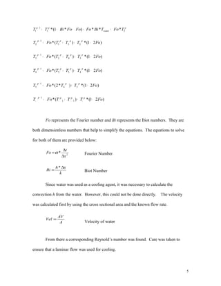
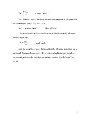
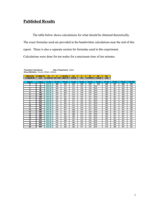
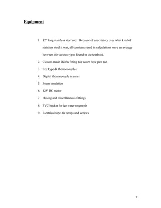
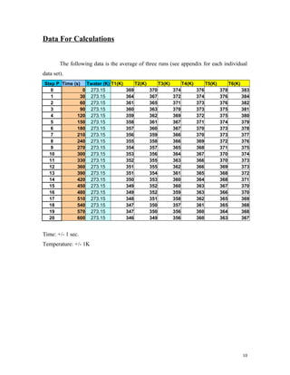
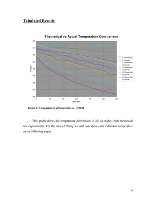
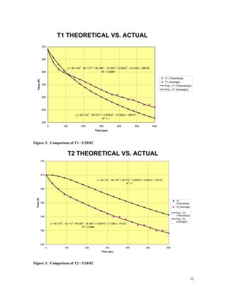
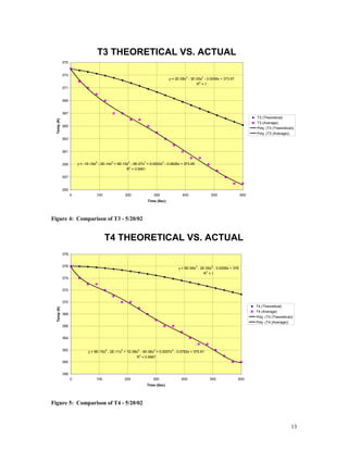
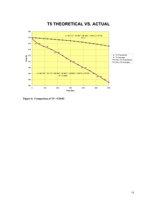
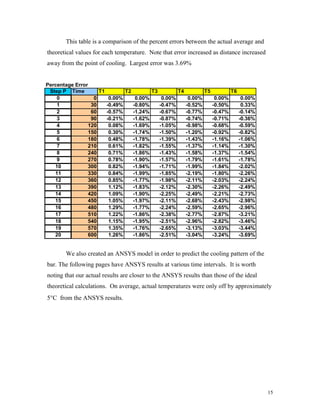
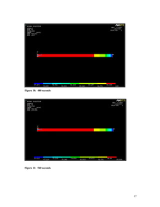
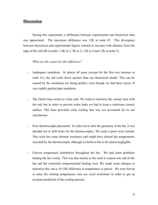
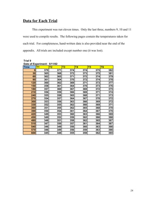
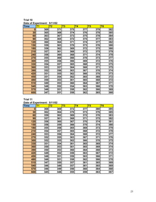
THERMO/FLUIDS LAB ME 415
Design Project:
Transient Heat Conduction
In a Semi-Infinite Plate
ME 415 Lab
Instructor: Dr. Ross
Group Members: Ezcurra, Johnson, Gibson
Date of Experiment: 5/6/02
Date of Report: 5/20/02
Ezcurra: pp 9-21
Johnson: pp 35-48 (all hand calculations), 11-18
Gibson: pp 1-8, 11-15, 23-25
TABLE OF CONTENTS
Page
Abstract 3
Theory 4
Published Results 7
Equipment 8
Procedure 9
Data for Calculations 10
Tabulated Results with Graphs 11
Discussion 18
Diagrams and Schematics 19
References 21
Equations Used 23
Data for Each Trial 24
Original Data Sheets 25
Original Hand Calculations 35
2
Abstract
In this lab, a stainless steel rod one foot in length was heated to 100°C and then
cooled with ice water. The ice water was pumped through a special fitting attached at
one end of the rod that cooled only the very end of the bar. Temperatures at five nodes
were taken in 30-second intervals up to ten minutes. Actual temperatures were closer to
theoretically values closer to the end of the bar with the fitting. Temperatures digressed
more at further nodes. The maximum difference between theoretical and actual
temperatures was approximately 12K. More detailed results are provided in the
Tabulated Results section of this report.
3
Theory
Under certain circumstances a bar of steel only 12” can act theoretically as if it
were infinite in length. This rod can be considered semi-infinite in length because it
provides the practicality of simulating situations where a variable, such as temperature in
this case, would need to be considered over an infinite length. Despite our rod only being
12” long, it is theoretically similar to a rod of infinite length. This allows us to accurately
estimate the temperature distribution throughout the entire rod over a period of time.
Temperature distribution was calculated using the finite element method. The bar
was divided into ten nodes, each with identical lengths. Each node has a formula to
calculate its temperature depending on both the node after it and before it. In other
words, one cannot calculate the temperature at one point without analyzing temperatures
before and past the point. To prevent a perpetual loop of calculations, the last node is
counted twice so that one does not need to perform an infinite amount of calculations.
Although this method works well, it does have a disadvantage in that a stability
requirement must be met. Usually a very small or uneven time interval must be used in
order to use finite element analysis. The time interval for this experiment was only 30
seconds making recording temperature values a bit of a challenge.
Even though calculations were done with ten nodes, only the first five were
considered for analysis. A sixth thermocouple was added to the end opposite to the
fitting where cooling was taking place to ensure we had an infinite rod. The five
equations shown on the proceeding page were used to calculate the temperatures for the
first five nodes.
4
Fo represents the Fourier number and Bi represents the Biot numbers. They are
both dimensionless numbers that help to simplify the equations. The equations to solve
for both of them are provided below:
2
*
x
t
Fo
∆
∆
=α Fourier Number
k
xh
Bi
∆
=
*
Biot Number
Since water was used as a cooling agent, it was necessary to calculate the
convection h from the water. However, this could not be done directly. The velocity
was calculated first by using the cross sectional area and the known flow rate.
A
AV
Vel
.
=
Velocity of water
From there a corresponding Reynold’s number was found. Care was taken to
ensure that a laminar flow was used for cooling.
5
)21(*)(*
)21(*)*2(*
)21(*)(*
)21(*)(*
)21(*)(*
11
1
54
1
5
453
1
4
342
1
3
231
1
2
FoTTTFoT
FoTTFoT
FoTTTFoT
FoTTTFoT
FoTTTFoT
pppp
ppp
pppp
pppp
pppp
−++=
−+=
−++=
−++=
−++=
∞+∞−∞
+
∞
+
+
+
+
p
water
pp
TFoTBiFoFoFoBiTT 21
1
1 ***)*1(* ++−−=+
ν
hDV *
Re = Reynold’s Number
Once Reynold’s number was found, the Nusselt number could be calculated using
the known Prandtl number from the textbook.
3/12/1
_
Pr*Re*664.=extNu Nusselt Number
Convection can then be determined knowing the Nusselt number by solving the
below equation for h.
fluidK
Lh
Nu
*_
= Nusselt Number
Once the convection is known than calculations for estimating temperature can be
performed. Hand calculations are provided in the appendix of this report. Complete
spreadsheet calculations for each of the ten nodes are provided in the Tabulated Data
section
6
Published Results
The table below shows calculations for what should be obtained theoretically.
The exact formulae used are provided in the handwritten calculations near the end of this
report. There is also a separate section for formulae used in this experiment.
Calculations were done for ten nodes for a maximum time of ten minutes.
7
Theoretical Calculations Date of Experiment: 5/6/02
Group Members: Ezcurra, Gibson, Johnson
diffusivity L=delta X Fo h density Cp k Bi Re Nu
3.75944E-06 0.03 0.125315 133.7148 8042.75 476.25 14.4 0.278572 1724.80 3.66
Step P T (sec) To (K) T1 (K) T2 (K) T3 (K) T4 (K) T5 (K) T6 (K) T7 (K) T8 (K) T9 (K) T10 (K)
0 0 273.15 369 370 374 376 378 379 380 381 382 383
1 30 273.15 366 370 374 376 378 379 380 381 382 383
2 60 273.15 363 370 374 376 378 379 380 381 382 383
3 90 273.15 361 369 373 376 378 379 380 381 382 382
4 120 273.15 359 368 373 376 378 379 380 381 382 382
5 150 273.15 357 367 373 376 377 379 380 381 382 382
6 180 273.15 355 367 372 375 377 379 380 381 382 382
7 210 273.15 354 366 372 375 377 379 380 381 382 382
8 240 273.15 353 365 371 375 377 379 380 381 382 382
9 270 273.15 351 364 371 375 377 379 380 381 382 382
10 300 273.15 350 363 370 374 377 379 380 381 381 382
11 330 273.15 349 362 370 374 377 379 380 381 381 382
12 360 273.15 348 361 369 374 377 378 380 381 381 382
13 390 273.15 347 361 369 374 376 378 380 381 381 381
14 420 273.15 346 360 368 373 376 378 380 381 381 381
15 450 273.15 345 359 368 373 376 378 380 381 381 381
16 480 273.15 345 358 367 373 376 378 380 381 381 381
17 510 273.15 344 358 367 372 376 378 379 380 381 381
18 540 273.15 343 357 366 372 376 378 379 380 381 381
19 570 273.15 342 356 366 372 375 378 379 380 381 381
20 600 273.15 342 356 365 371 375 378 379 380 381 381
Equipment
1. 12” long stainless steel rod. Because of uncertainty over what kind of
stainless steel it was, all constants used in calculations were an average
between the various types found in the textbook.
2. Custom made Delrin fitting for water flow past rod
3. Six Type-K thermocouples
4. Digital thermocouple scanner
5. Foam insulation
6. 12V DC motor
7. Hosing and miscellaneous fittings
8. PVC bucket for ice water reservoir
9. Electrical tape, tie wraps and screws
8
Procedure
The following steps were followed:
1. Connect all thermocouples to the scanner.
2. Remove rod assembly from Delrin base (to facilitate even heating)
3. Turn the heating wire on (power supply set at 75)
4. Heat the bar until all thermocouples register 400K
5. Allow the bar to cool down until thermocouple #1 reads 373K (by this time
temperature in the bar should have stabilized)
6. Insert the bar in the Delrin base and fill the reservoir with ice water.
7. Turn pump on (power supply set at 5V)
8. Start recording all six temperatures every 30 seconds for 10 minutes.
9
Data For Calculations
The following data is the average of three runs (see appendix for each individual
data set).
Step P Time (s) Twater (K) T1(K) T2(K) T3(K) T4(K) T5(K) T6(K)
0 0 273.15 369 370 374 376 378 383
1 30 273.15 364 367 372 374 376 384
2 60 273.15 361 365 371 373 376 382
3 90 273.15 360 363 370 373 375 381
4 120 273.15 359 362 369 372 375 380
5 150 273.15 358 361 367 371 374 379
6 180 273.15 357 360 367 370 373 378
7 210 273.15 356 359 366 370 373 377
8 240 273.15 355 358 366 369 372 376
9 270 273.15 354 357 365 368 371 375
10 300 273.15 353 356 364 367 370 374
11 330 273.15 352 355 363 366 370 373
12 360 273.15 351 355 362 366 369 373
13 390 273.15 351 354 361 365 368 372
14 420 273.15 350 353 360 364 368 371
15 450 273.15 349 352 360 363 367 370
16 480 273.15 349 352 359 363 366 370
17 510 273.15 348 351 358 362 365 369
18 540 273.15 347 350 357 361 365 368
19 570 273.15 347 350 356 360 364 368
20 600 273.15 346 349 356 360 363 367
Time: +/- 1 sec.
Temperature: +/- 1K
10
Tabulated Results
This graph shows the temperature distribution of all six nodes, both theoretical
and experimental. For the sake of clarity we will now show each individual temperature
on the following pages.
11
Theoretical vs Actual Temperature Comparison
340
345
350
355
360
365
370
375
380
0 100 200 300 400 500 600
Time (sec)
Temp(K)
T1 (Theoretical)
T1 (Actual)
T2 (Theoretical)
T2 (Actual)
T3 (Theoretical)
T3 (Actual)
T4 (Theoretical)
T4 (Actual)
T5 (Theoretical)
T5 (Actual)
Figure 1: Comparison of all temperatures – 5/20/02
T1 THEORETICAL VS. ACTUAL
y = 2E-10x4
- 3E-07x3
+ 0.0002x2
- 0.1092x + 368.91
R2
= 1
y = 2E-14x
6
- 3E-11x
5
+ 3E-08x
4
- 1E-05x
3
+ 0.002x
2
- 0.2142x + 368.93
R
2
= 0.9987
340
345
350
355
360
365
370
0 100 200 300 400 500 600
Time (sec)
Temp(K)
T1 (Theoretical)
T1 (Average)
Poly. (T1 (Theoretical))
Poly. (T1 (Average))
Figure 2: Comparison of T1 - 5/20/02
T2 THEORETICAL VS. ACTUAL
y = 5E-13x
5
- 9E-10x
4
+ 6E-07x
3
- 0.0002x
2
+ 0.0027x + 370.03
R
2
= 1
y = 5E-15x
6
- 1E-11x
5
+ 8E-09x
4
- 3E-06x
3
+ 0.0007x
2
- 0.1206x + 370.02
R
2
= 0.9986
345
350
355
360
365
370
375
0 100 200 300 400 500 600
Time (sec)
Temp(K)
T2
(Theoretical)
T2 (Average)
Poly. (T2
(Theoretical))
Poly. (T2
(Average))
Figure 3: Comparison of T2 - 5/20/02
12
T3 THEORETICAL VS. ACTUAL
y = 2E-08x
3
- 3E-05x
2
- 0.0058x + 373.97
R
2
= 1
y = -1E-16x
6
- 2E-14x
5
+ 5E-10x
4
- 5E-07x
3
+ 0.0002x
2
- 0.0626x + 373.95
R
2
= 0.9961
355
357
359
361
363
365
367
369
371
373
375
0 100 200 300 400 500 600
Time (Sec)
Temp(K)
T3 (Theoretical)
T3 (Average)
Poly. (T3 (Theoretical))
Poly. (T3 (Average))
Figure 4: Comparison of T3 - 5/20/02
T4 THEORETICAL VS. ACTUAL
y = 9E-09x
3
- 2E-05x
2
- 0.0008x + 376
R
2
= 1
y = 9E-15x
6
- 2E-11x
5
+ 1E-08x
4
- 4E-06x
3
+ 0.0007x
2
- 0.0752x + 375.91
R
2
= 0.9967
358
360
362
364
366
368
370
372
374
376
378
0 100 200 300 400 500 600
Time (Sec)
Temp(K)
T4 (Theoretical)
T4 (Average)
Poly. (T4 (Theoretical))
Poly. (T4 (Average))
Figure 5: Comparison of T4 - 5/20/02
13
T5 THEORETICAL VS. ACTUAL
y = 2E-11x
4
- 3E-08x
3
+ 8E-06x
2
- 0.0041x + 377.99
R
2
= 1
y = 6E-15x
6
- 1E-11x
5
+ 9E-09x
4
- 3E-06x
3
+ 0.0005x
2
- 0.0577x + 377.82
R
2
= 0.9955
362
364
366
368
370
372
374
376
378
380
0 100 200 300 400 500 600
Time (Sec)
Temp(K)
T5 (Theoretical)
T5 (Average)
Poly. (T5 (Theoretical))
Poly. (T5 (Average))
Figure 6: Comparison of T5 - 5/20/02
14
This table is a comparison of the percent errors between the actual average and
theoretical values for each temperature. Note that error increased as distance increased
away from the point of cooling. Largest error was 3.69%
We also created an ANSYS model in order to predict the cooling pattern of the
bar. The following pages have ANSYS results at various time intervals. It is worth
noting that our actual results are closer to the ANSYS results than those of the ideal
theoretical calculations. On average, actual temperatures were only off by approximately
5°C from the ANSYS results.
15
Percentage Error
Step P Time T1 T2 T3 T4 T5 T6
0 0 0.00% 0.00% 0.00% 0.00% 0.00% 0.00%
1 30 -0.49% -0.80% -0.47% -0.52% -0.50% 0.33%
2 60 -0.57% -1.24% -0.67% -0.77% -0.47% -0.14%
3 90 -0.21% -1.62% -0.87% -0.74% -0.71% -0.36%
4 120 0.08% -1.69% -1.05% -0.98% -0.68% -0.59%
5 150 0.30% -1.74% -1.50% -1.20% -0.92% -0.82%
6 180 0.48% -1.78% -1.39% -1.43% -1.16% -1.06%
7 210 0.61% -1.82% -1.55% -1.37% -1.14% -1.30%
8 240 0.71% -1.86% -1.43% -1.58% -1.37% -1.54%
9 270 0.78% -1.90% -1.57% -1.79% -1.61% -1.78%
10 300 0.82% -1.94% -1.71% -1.99% -1.84% -2.02%
11 330 0.84% -1.99% -1.85% -2.19% -1.80% -2.26%
12 360 0.85% -1.77% -1.98% -2.11% -2.03% -2.24%
13 390 1.12% -1.83% -2.12% -2.30% -2.26% -2.49%
14 420 1.09% -1.90% -2.25% -2.49% -2.21% -2.73%
15 450 1.05% -1.97% -2.11% -2.68% -2.43% -2.98%
16 480 1.29% -1.77% -2.24% -2.59% -2.65% -2.96%
17 510 1.22% -1.86% -2.38% -2.77% -2.87% -3.21%
18 540 1.15% -1.95% -2.51% -2.96% -2.82% -3.46%
19 570 1.35% -1.76% -2.65% -3.13% -3.03% -3.44%
20 600 1.26% -1.86% -2.51% -3.04% -3.24% -3.69%
Time: 240 sec
16
Figure 7: 60 seconds
Figure 9: 240 seconds
Figure 8: 480 seconds
17
Figure 11: 540 seconds
Figure 10: 480 seconds
Discussion
During this experiment, a difference between experimental and theoretical data
was appreciated. The maximum difference was 12K in node #5. This divergence
between theoretical and experimental figures seemed to increase with distance from the
edge of the rod (4K in node 1, 6K in 2, 7K in 3, 11K in 4 and 12K in node 5).
What are the causes for this difference?
- Inadequate insulation: In almost all cases (except for the first two minutes in
node #1), the rod cools down quicker than our theoretical model. This can be
caused by the insulation not being perfect, even though we had three layers of
very tightly packed pipe insulation.
- The Delrin base acted as a heat sink. We tried to minimize the contact area with
the rod, but in order to prevent water leaks we had to keep a minimum contact
surface. This base provided extra cooling that was not accounted for in our
calculations.
- Poor thermocouple placement: In order not to alter the geometry of the bar, it was
decided not to drill holes for the thermocouples. We used a epoxi resin instead.
This resin has some thermal resistance and might have altered the temperatures
recorded by the thermocouple, although we believe this to be almost negligible.
- Uneven temperature distribution throughout the bar: We had some problems
heating the bar evenly. This was due mainly to the need to expose one end of the
bar and the somewhat temperamental heating wire. We made some changes to
minimize this, but a 10-15K difference in temperature is typical. We were forced
to enter the starting temperatures into our excel worksheet in order to get an
accurate prediction of the cooling process.
18
Diagrams and Schematics
19
h
INSULATION
INSULATION
T10T5T4T3T2T1
HEATING WIREdx
12in
Ice water Pump
Heating wire
Thermocouples
Thermocouple scanner
Power supply
(for heating wire)
Power supply
(for pump)
EXPERIMENT SETUP
Rod
Insulation
Figure 12: Diagram showing nodes and point of convection
Figure 13: Schematic of setup
20
Figure 14: Photo of project from front
Cold water
h
Stainless steel rod
Insulation
Delrin water
enclosure
Figure 15: Cutaway of fitting for rod. Note that bored hole is larger than hole for rod.
References
1. Fundamentals of Heat and Mass Transfer: 4th
Edition. Incropera and DeWitt,
1996.
2. ME415 Lab manual
3. ME 404 class notes
4. ANSYS manual. Version 5.7, 1998
5. Fundamentals of Heat and Mass Transfer: 2nd
Edition. Incropera and DeWitt,
1985.
21
Appendix
22
Equations Used
A
AV
Vel
.
=
ν
LV *
Re =
ν
hDV *
Re =
P
A
Dh
*4
=
ba
ba
Dh
+
=
**2
3/12/1
_
Pr*Re*664.=extNu
66.3
_
int =Nu
fluidK
Lh
Nu
*_
=
Cp
K
*ρ
α =
k
xh
Bi
∆
=
*
2
*
x
t
Fo
∆
∆
=α
∑ ∆
∆
=+
t
T
CpmQQ genconvcond **/
t
T
CpmQQ condconv
∆
∆
=+ **
x
TAk
q
TAhq
∆
∆
=
∆=
)(*
)(**
Vel. = velocity
AV = volumetric flow rate
Re = Reynolds number
V = velocity
L = length
Dh = hydraulic diameter
P = perimeter
a = height
b = width
Nu = Nusselt number
Pr = Prandtl number
h = convection heat transfer coefficient
k = thermal conductivity
ρ = density
Cp = specific heat
α = diffusivity
Bi = Biot number
Fo = Fourier number
Energy balance equation:
m = mass
T = temperature
T = time
Q = energy transfer
q = heat transfer
23
Data for Each Trial
This experiment was run eleven times. Only the last three, numbers 9, 10 and 11
were used to compile results. The following pages contain the temperatures taken for
each trial. For completeness, hand-written data is also provided near the end of the
appendix. All trials are included except number one (it was lost).
24
Trial 9
Date of Experiment: 5/11/02
Time T1 T2 T3 T4 T5 T6
0 370 371 374 374 375 382
30 365 368 372 373 375 381
60 362 365 371 372 374 379
90 361 364 370 372 374 378
120 360 362 369 371 373 377
150 358 361 364 370 373 376
180 357 360 367 369 372 375
210 356 359 366 369 371 374
240 355 358 365 368 371 373
270 354 357 364 367 370 372
300 353 356 363 366 369 372
330 352 355 362 366 369 371
360 351 355 362 365 368 370
390 350 354 361 364 367 370
420 349 353 360 363 366 369
450 349 352 359 362 366 368
480 348 351 358 362 365 367
510 347 350 357 361 364 367
540 346 349 356 360 363 366
570 346 349 356 359 363 366
600 345 348 355 359 362 365
25
Trial 10
Date of Experiment: 5/11/02
Time T1 T2 T3 T4 T5 T6
0 369 371 375 377 379 382
30 365 368 374 376 378 385
60 363 367 373 375 378 384
90 362 365 372 375 377 383
120 360 364 371 374 377 382
150 359 363 370 373 376 380
180 358 362 369 372 375 380
210 357 361 368 372 375 379
240 356 360 368 371 374 378
270 355 369 366 370 373 377
300 355 358 366 369 372 376
330 354 357 365 368 372 375
360 353 357 364 368 371 375
390 352 356 363 367 370 374
420 351 355 362 366 370 373
450 351 354 362 365 369 372
480 350 353 361 365 368 372
510 349 353 360 364 367 371
540 348 352 354 363 366 370
570 348 351 358 362 366 369
600 347 351 358 362 365 368
Trial 11
Date of Experiment: 5/11/02
Time T1 T2 T3 T4 T5 T6
0 368 369 372 377 380 385
30 362 364 370 373 376 385
60 359 362 369 372 376 383
90 357 361 368 371 375 382
120 356 360 367 370 374 381
150 356 359 366 370 374 380
180 355 358 365 369 373 379
210 354 357 365 368 372 378
240 353 356 364 368 372 377
270 352 355 363 367 371 376
300 352 355 362 366 370 375
330 351 354 361 365 369 374
360 350 353 361 365 369 374
390 350 353 360 364 368 373
420 349 352 359 363 367 372
450 348 351 359 363 366 371
480 348 351 358 362 366 370
510 347 350 357 361 365 369
540 346 349 357 361 365 369
570 346 349 356 360 364 368
600 345 348 355 359 363 367

Jean-Paul Gibson: Transient Heat Conduction in a Semi-Infinite Plate Compared To ANSYS Values

  • 1.
    THERMO/FLUIDS LAB ME415 Design Project: Transient Heat Conduction In a Semi-Infinite Plate ME 415 Lab Instructor: Dr. Ross Group Members: Ezcurra, Johnson, Gibson Date of Experiment: 5/6/02 Date of Report: 5/20/02 Ezcurra: pp 9-21 Johnson: pp 35-48 (all hand calculations), 11-18 Gibson: pp 1-8, 11-15, 23-25
  • 2.
    TABLE OF CONTENTS Page Abstract3 Theory 4 Published Results 7 Equipment 8 Procedure 9 Data for Calculations 10 Tabulated Results with Graphs 11 Discussion 18 Diagrams and Schematics 19 References 21 Equations Used 23 Data for Each Trial 24 Original Data Sheets 25 Original Hand Calculations 35 2
  • 3.
    Abstract In this lab,a stainless steel rod one foot in length was heated to 100°C and then cooled with ice water. The ice water was pumped through a special fitting attached at one end of the rod that cooled only the very end of the bar. Temperatures at five nodes were taken in 30-second intervals up to ten minutes. Actual temperatures were closer to theoretically values closer to the end of the bar with the fitting. Temperatures digressed more at further nodes. The maximum difference between theoretical and actual temperatures was approximately 12K. More detailed results are provided in the Tabulated Results section of this report. 3
  • 4.
    Theory Under certain circumstancesa bar of steel only 12” can act theoretically as if it were infinite in length. This rod can be considered semi-infinite in length because it provides the practicality of simulating situations where a variable, such as temperature in this case, would need to be considered over an infinite length. Despite our rod only being 12” long, it is theoretically similar to a rod of infinite length. This allows us to accurately estimate the temperature distribution throughout the entire rod over a period of time. Temperature distribution was calculated using the finite element method. The bar was divided into ten nodes, each with identical lengths. Each node has a formula to calculate its temperature depending on both the node after it and before it. In other words, one cannot calculate the temperature at one point without analyzing temperatures before and past the point. To prevent a perpetual loop of calculations, the last node is counted twice so that one does not need to perform an infinite amount of calculations. Although this method works well, it does have a disadvantage in that a stability requirement must be met. Usually a very small or uneven time interval must be used in order to use finite element analysis. The time interval for this experiment was only 30 seconds making recording temperature values a bit of a challenge. Even though calculations were done with ten nodes, only the first five were considered for analysis. A sixth thermocouple was added to the end opposite to the fitting where cooling was taking place to ensure we had an infinite rod. The five equations shown on the proceeding page were used to calculate the temperatures for the first five nodes. 4
  • 5.
    Fo represents theFourier number and Bi represents the Biot numbers. They are both dimensionless numbers that help to simplify the equations. The equations to solve for both of them are provided below: 2 * x t Fo ∆ ∆ =α Fourier Number k xh Bi ∆ = * Biot Number Since water was used as a cooling agent, it was necessary to calculate the convection h from the water. However, this could not be done directly. The velocity was calculated first by using the cross sectional area and the known flow rate. A AV Vel . = Velocity of water From there a corresponding Reynold’s number was found. Care was taken to ensure that a laminar flow was used for cooling. 5 )21(*)(* )21(*)*2(* )21(*)(* )21(*)(* )21(*)(* 11 1 54 1 5 453 1 4 342 1 3 231 1 2 FoTTTFoT FoTTFoT FoTTTFoT FoTTTFoT FoTTTFoT pppp ppp pppp pppp pppp −++= −+= −++= −++= −++= ∞+∞−∞ + ∞ + + + + p water pp TFoTBiFoFoFoBiTT 21 1 1 ***)*1(* ++−−=+
  • 6.
    ν hDV * Re =Reynold’s Number Once Reynold’s number was found, the Nusselt number could be calculated using the known Prandtl number from the textbook. 3/12/1 _ Pr*Re*664.=extNu Nusselt Number Convection can then be determined knowing the Nusselt number by solving the below equation for h. fluidK Lh Nu *_ = Nusselt Number Once the convection is known than calculations for estimating temperature can be performed. Hand calculations are provided in the appendix of this report. Complete spreadsheet calculations for each of the ten nodes are provided in the Tabulated Data section 6
  • 7.
    Published Results The tablebelow shows calculations for what should be obtained theoretically. The exact formulae used are provided in the handwritten calculations near the end of this report. There is also a separate section for formulae used in this experiment. Calculations were done for ten nodes for a maximum time of ten minutes. 7 Theoretical Calculations Date of Experiment: 5/6/02 Group Members: Ezcurra, Gibson, Johnson diffusivity L=delta X Fo h density Cp k Bi Re Nu 3.75944E-06 0.03 0.125315 133.7148 8042.75 476.25 14.4 0.278572 1724.80 3.66 Step P T (sec) To (K) T1 (K) T2 (K) T3 (K) T4 (K) T5 (K) T6 (K) T7 (K) T8 (K) T9 (K) T10 (K) 0 0 273.15 369 370 374 376 378 379 380 381 382 383 1 30 273.15 366 370 374 376 378 379 380 381 382 383 2 60 273.15 363 370 374 376 378 379 380 381 382 383 3 90 273.15 361 369 373 376 378 379 380 381 382 382 4 120 273.15 359 368 373 376 378 379 380 381 382 382 5 150 273.15 357 367 373 376 377 379 380 381 382 382 6 180 273.15 355 367 372 375 377 379 380 381 382 382 7 210 273.15 354 366 372 375 377 379 380 381 382 382 8 240 273.15 353 365 371 375 377 379 380 381 382 382 9 270 273.15 351 364 371 375 377 379 380 381 382 382 10 300 273.15 350 363 370 374 377 379 380 381 381 382 11 330 273.15 349 362 370 374 377 379 380 381 381 382 12 360 273.15 348 361 369 374 377 378 380 381 381 382 13 390 273.15 347 361 369 374 376 378 380 381 381 381 14 420 273.15 346 360 368 373 376 378 380 381 381 381 15 450 273.15 345 359 368 373 376 378 380 381 381 381 16 480 273.15 345 358 367 373 376 378 380 381 381 381 17 510 273.15 344 358 367 372 376 378 379 380 381 381 18 540 273.15 343 357 366 372 376 378 379 380 381 381 19 570 273.15 342 356 366 372 375 378 379 380 381 381 20 600 273.15 342 356 365 371 375 378 379 380 381 381
  • 8.
    Equipment 1. 12” longstainless steel rod. Because of uncertainty over what kind of stainless steel it was, all constants used in calculations were an average between the various types found in the textbook. 2. Custom made Delrin fitting for water flow past rod 3. Six Type-K thermocouples 4. Digital thermocouple scanner 5. Foam insulation 6. 12V DC motor 7. Hosing and miscellaneous fittings 8. PVC bucket for ice water reservoir 9. Electrical tape, tie wraps and screws 8
  • 9.
    Procedure The following stepswere followed: 1. Connect all thermocouples to the scanner. 2. Remove rod assembly from Delrin base (to facilitate even heating) 3. Turn the heating wire on (power supply set at 75) 4. Heat the bar until all thermocouples register 400K 5. Allow the bar to cool down until thermocouple #1 reads 373K (by this time temperature in the bar should have stabilized) 6. Insert the bar in the Delrin base and fill the reservoir with ice water. 7. Turn pump on (power supply set at 5V) 8. Start recording all six temperatures every 30 seconds for 10 minutes. 9
  • 10.
    Data For Calculations Thefollowing data is the average of three runs (see appendix for each individual data set). Step P Time (s) Twater (K) T1(K) T2(K) T3(K) T4(K) T5(K) T6(K) 0 0 273.15 369 370 374 376 378 383 1 30 273.15 364 367 372 374 376 384 2 60 273.15 361 365 371 373 376 382 3 90 273.15 360 363 370 373 375 381 4 120 273.15 359 362 369 372 375 380 5 150 273.15 358 361 367 371 374 379 6 180 273.15 357 360 367 370 373 378 7 210 273.15 356 359 366 370 373 377 8 240 273.15 355 358 366 369 372 376 9 270 273.15 354 357 365 368 371 375 10 300 273.15 353 356 364 367 370 374 11 330 273.15 352 355 363 366 370 373 12 360 273.15 351 355 362 366 369 373 13 390 273.15 351 354 361 365 368 372 14 420 273.15 350 353 360 364 368 371 15 450 273.15 349 352 360 363 367 370 16 480 273.15 349 352 359 363 366 370 17 510 273.15 348 351 358 362 365 369 18 540 273.15 347 350 357 361 365 368 19 570 273.15 347 350 356 360 364 368 20 600 273.15 346 349 356 360 363 367 Time: +/- 1 sec. Temperature: +/- 1K 10
  • 11.
    Tabulated Results This graphshows the temperature distribution of all six nodes, both theoretical and experimental. For the sake of clarity we will now show each individual temperature on the following pages. 11 Theoretical vs Actual Temperature Comparison 340 345 350 355 360 365 370 375 380 0 100 200 300 400 500 600 Time (sec) Temp(K) T1 (Theoretical) T1 (Actual) T2 (Theoretical) T2 (Actual) T3 (Theoretical) T3 (Actual) T4 (Theoretical) T4 (Actual) T5 (Theoretical) T5 (Actual) Figure 1: Comparison of all temperatures – 5/20/02
  • 12.
    T1 THEORETICAL VS.ACTUAL y = 2E-10x4 - 3E-07x3 + 0.0002x2 - 0.1092x + 368.91 R2 = 1 y = 2E-14x 6 - 3E-11x 5 + 3E-08x 4 - 1E-05x 3 + 0.002x 2 - 0.2142x + 368.93 R 2 = 0.9987 340 345 350 355 360 365 370 0 100 200 300 400 500 600 Time (sec) Temp(K) T1 (Theoretical) T1 (Average) Poly. (T1 (Theoretical)) Poly. (T1 (Average)) Figure 2: Comparison of T1 - 5/20/02 T2 THEORETICAL VS. ACTUAL y = 5E-13x 5 - 9E-10x 4 + 6E-07x 3 - 0.0002x 2 + 0.0027x + 370.03 R 2 = 1 y = 5E-15x 6 - 1E-11x 5 + 8E-09x 4 - 3E-06x 3 + 0.0007x 2 - 0.1206x + 370.02 R 2 = 0.9986 345 350 355 360 365 370 375 0 100 200 300 400 500 600 Time (sec) Temp(K) T2 (Theoretical) T2 (Average) Poly. (T2 (Theoretical)) Poly. (T2 (Average)) Figure 3: Comparison of T2 - 5/20/02 12
  • 13.
    T3 THEORETICAL VS.ACTUAL y = 2E-08x 3 - 3E-05x 2 - 0.0058x + 373.97 R 2 = 1 y = -1E-16x 6 - 2E-14x 5 + 5E-10x 4 - 5E-07x 3 + 0.0002x 2 - 0.0626x + 373.95 R 2 = 0.9961 355 357 359 361 363 365 367 369 371 373 375 0 100 200 300 400 500 600 Time (Sec) Temp(K) T3 (Theoretical) T3 (Average) Poly. (T3 (Theoretical)) Poly. (T3 (Average)) Figure 4: Comparison of T3 - 5/20/02 T4 THEORETICAL VS. ACTUAL y = 9E-09x 3 - 2E-05x 2 - 0.0008x + 376 R 2 = 1 y = 9E-15x 6 - 2E-11x 5 + 1E-08x 4 - 4E-06x 3 + 0.0007x 2 - 0.0752x + 375.91 R 2 = 0.9967 358 360 362 364 366 368 370 372 374 376 378 0 100 200 300 400 500 600 Time (Sec) Temp(K) T4 (Theoretical) T4 (Average) Poly. (T4 (Theoretical)) Poly. (T4 (Average)) Figure 5: Comparison of T4 - 5/20/02 13
  • 14.
    T5 THEORETICAL VS.ACTUAL y = 2E-11x 4 - 3E-08x 3 + 8E-06x 2 - 0.0041x + 377.99 R 2 = 1 y = 6E-15x 6 - 1E-11x 5 + 9E-09x 4 - 3E-06x 3 + 0.0005x 2 - 0.0577x + 377.82 R 2 = 0.9955 362 364 366 368 370 372 374 376 378 380 0 100 200 300 400 500 600 Time (Sec) Temp(K) T5 (Theoretical) T5 (Average) Poly. (T5 (Theoretical)) Poly. (T5 (Average)) Figure 6: Comparison of T5 - 5/20/02 14
  • 15.
    This table isa comparison of the percent errors between the actual average and theoretical values for each temperature. Note that error increased as distance increased away from the point of cooling. Largest error was 3.69% We also created an ANSYS model in order to predict the cooling pattern of the bar. The following pages have ANSYS results at various time intervals. It is worth noting that our actual results are closer to the ANSYS results than those of the ideal theoretical calculations. On average, actual temperatures were only off by approximately 5°C from the ANSYS results. 15 Percentage Error Step P Time T1 T2 T3 T4 T5 T6 0 0 0.00% 0.00% 0.00% 0.00% 0.00% 0.00% 1 30 -0.49% -0.80% -0.47% -0.52% -0.50% 0.33% 2 60 -0.57% -1.24% -0.67% -0.77% -0.47% -0.14% 3 90 -0.21% -1.62% -0.87% -0.74% -0.71% -0.36% 4 120 0.08% -1.69% -1.05% -0.98% -0.68% -0.59% 5 150 0.30% -1.74% -1.50% -1.20% -0.92% -0.82% 6 180 0.48% -1.78% -1.39% -1.43% -1.16% -1.06% 7 210 0.61% -1.82% -1.55% -1.37% -1.14% -1.30% 8 240 0.71% -1.86% -1.43% -1.58% -1.37% -1.54% 9 270 0.78% -1.90% -1.57% -1.79% -1.61% -1.78% 10 300 0.82% -1.94% -1.71% -1.99% -1.84% -2.02% 11 330 0.84% -1.99% -1.85% -2.19% -1.80% -2.26% 12 360 0.85% -1.77% -1.98% -2.11% -2.03% -2.24% 13 390 1.12% -1.83% -2.12% -2.30% -2.26% -2.49% 14 420 1.09% -1.90% -2.25% -2.49% -2.21% -2.73% 15 450 1.05% -1.97% -2.11% -2.68% -2.43% -2.98% 16 480 1.29% -1.77% -2.24% -2.59% -2.65% -2.96% 17 510 1.22% -1.86% -2.38% -2.77% -2.87% -3.21% 18 540 1.15% -1.95% -2.51% -2.96% -2.82% -3.46% 19 570 1.35% -1.76% -2.65% -3.13% -3.03% -3.44% 20 600 1.26% -1.86% -2.51% -3.04% -3.24% -3.69%
  • 16.
    Time: 240 sec 16 Figure7: 60 seconds Figure 9: 240 seconds Figure 8: 480 seconds
  • 17.
    17 Figure 11: 540seconds Figure 10: 480 seconds
  • 18.
    Discussion During this experiment,a difference between experimental and theoretical data was appreciated. The maximum difference was 12K in node #5. This divergence between theoretical and experimental figures seemed to increase with distance from the edge of the rod (4K in node 1, 6K in 2, 7K in 3, 11K in 4 and 12K in node 5). What are the causes for this difference? - Inadequate insulation: In almost all cases (except for the first two minutes in node #1), the rod cools down quicker than our theoretical model. This can be caused by the insulation not being perfect, even though we had three layers of very tightly packed pipe insulation. - The Delrin base acted as a heat sink. We tried to minimize the contact area with the rod, but in order to prevent water leaks we had to keep a minimum contact surface. This base provided extra cooling that was not accounted for in our calculations. - Poor thermocouple placement: In order not to alter the geometry of the bar, it was decided not to drill holes for the thermocouples. We used a epoxi resin instead. This resin has some thermal resistance and might have altered the temperatures recorded by the thermocouple, although we believe this to be almost negligible. - Uneven temperature distribution throughout the bar: We had some problems heating the bar evenly. This was due mainly to the need to expose one end of the bar and the somewhat temperamental heating wire. We made some changes to minimize this, but a 10-15K difference in temperature is typical. We were forced to enter the starting temperatures into our excel worksheet in order to get an accurate prediction of the cooling process. 18
  • 19.
    Diagrams and Schematics 19 h INSULATION INSULATION T10T5T4T3T2T1 HEATINGWIREdx 12in Ice water Pump Heating wire Thermocouples Thermocouple scanner Power supply (for heating wire) Power supply (for pump) EXPERIMENT SETUP Rod Insulation Figure 12: Diagram showing nodes and point of convection Figure 13: Schematic of setup
  • 20.
    20 Figure 14: Photoof project from front Cold water h Stainless steel rod Insulation Delrin water enclosure Figure 15: Cutaway of fitting for rod. Note that bored hole is larger than hole for rod.
  • 21.
    References 1. Fundamentals ofHeat and Mass Transfer: 4th Edition. Incropera and DeWitt, 1996. 2. ME415 Lab manual 3. ME 404 class notes 4. ANSYS manual. Version 5.7, 1998 5. Fundamentals of Heat and Mass Transfer: 2nd Edition. Incropera and DeWitt, 1985. 21
  • 22.
  • 23.
    Equations Used A AV Vel . = ν LV * Re= ν hDV * Re = P A Dh *4 = ba ba Dh + = **2 3/12/1 _ Pr*Re*664.=extNu 66.3 _ int =Nu fluidK Lh Nu *_ = Cp K *ρ α = k xh Bi ∆ = * 2 * x t Fo ∆ ∆ =α ∑ ∆ ∆ =+ t T CpmQQ genconvcond **/ t T CpmQQ condconv ∆ ∆ =+ ** x TAk q TAhq ∆ ∆ = ∆= )(* )(** Vel. = velocity AV = volumetric flow rate Re = Reynolds number V = velocity L = length Dh = hydraulic diameter P = perimeter a = height b = width Nu = Nusselt number Pr = Prandtl number h = convection heat transfer coefficient k = thermal conductivity ρ = density Cp = specific heat α = diffusivity Bi = Biot number Fo = Fourier number Energy balance equation: m = mass T = temperature T = time Q = energy transfer q = heat transfer 23
  • 24.
    Data for EachTrial This experiment was run eleven times. Only the last three, numbers 9, 10 and 11 were used to compile results. The following pages contain the temperatures taken for each trial. For completeness, hand-written data is also provided near the end of the appendix. All trials are included except number one (it was lost). 24 Trial 9 Date of Experiment: 5/11/02 Time T1 T2 T3 T4 T5 T6 0 370 371 374 374 375 382 30 365 368 372 373 375 381 60 362 365 371 372 374 379 90 361 364 370 372 374 378 120 360 362 369 371 373 377 150 358 361 364 370 373 376 180 357 360 367 369 372 375 210 356 359 366 369 371 374 240 355 358 365 368 371 373 270 354 357 364 367 370 372 300 353 356 363 366 369 372 330 352 355 362 366 369 371 360 351 355 362 365 368 370 390 350 354 361 364 367 370 420 349 353 360 363 366 369 450 349 352 359 362 366 368 480 348 351 358 362 365 367 510 347 350 357 361 364 367 540 346 349 356 360 363 366 570 346 349 356 359 363 366 600 345 348 355 359 362 365
  • 25.
    25 Trial 10 Date ofExperiment: 5/11/02 Time T1 T2 T3 T4 T5 T6 0 369 371 375 377 379 382 30 365 368 374 376 378 385 60 363 367 373 375 378 384 90 362 365 372 375 377 383 120 360 364 371 374 377 382 150 359 363 370 373 376 380 180 358 362 369 372 375 380 210 357 361 368 372 375 379 240 356 360 368 371 374 378 270 355 369 366 370 373 377 300 355 358 366 369 372 376 330 354 357 365 368 372 375 360 353 357 364 368 371 375 390 352 356 363 367 370 374 420 351 355 362 366 370 373 450 351 354 362 365 369 372 480 350 353 361 365 368 372 510 349 353 360 364 367 371 540 348 352 354 363 366 370 570 348 351 358 362 366 369 600 347 351 358 362 365 368 Trial 11 Date of Experiment: 5/11/02 Time T1 T2 T3 T4 T5 T6 0 368 369 372 377 380 385 30 362 364 370 373 376 385 60 359 362 369 372 376 383 90 357 361 368 371 375 382 120 356 360 367 370 374 381 150 356 359 366 370 374 380 180 355 358 365 369 373 379 210 354 357 365 368 372 378 240 353 356 364 368 372 377 270 352 355 363 367 371 376 300 352 355 362 366 370 375 330 351 354 361 365 369 374 360 350 353 361 365 369 374 390 350 353 360 364 368 373 420 349 352 359 363 367 372 450 348 351 359 363 366 371 480 348 351 358 362 366 370 510 347 350 357 361 365 369 540 346 349 357 361 365 369 570 346 349 356 360 364 368 600 345 348 355 359 363 367