The document describes an experiment to model a pipe heat exchanger that cools water as it passes through a tub of ice. The student measured the inlet and outlet temperatures of water running through a garden hose submerged in an ice bath. The outlet temperature reached a steady state of 17 degrees Celsius within 4 seconds. Modeling with finite differences predicted a steady state of 10.5 degrees Celsius, showing a difference from the experimental results. Decreasing the mass flow rate through the pipe could achieve lower outlet temperatures by allowing more time for heat transfer. Suggestions for improving the experiment included not pre-cooling the hose and using software to better model heat transfer.

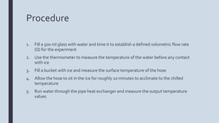
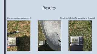
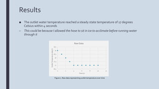
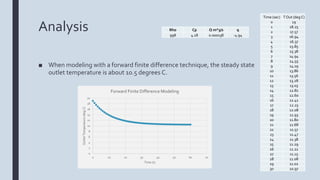
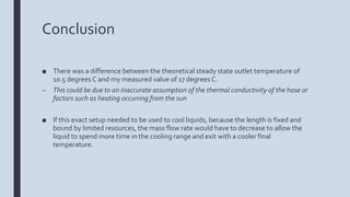
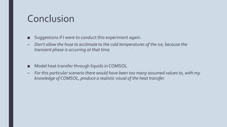
1. PIPE HEAT EXCHANGER
TyWilliams
BE 4120

2. Introduction/Objective
■ Objective: create and model a pipe heat exchanger that affectively cools water as it
passes through a tub of ice
■ To do so, I built a pipe heat exchanger with a constant surface temperature and
analyzed the results
■ Real world comparison: cooling wort sustainably as a part of the beer-making process

3. Materials
■ Tin bath
■ Ice
■ Measuring cup
■ Tape measure
■ Thermometer
■ Stop watch
■ Garden Hose (pipe)

4. Parameters
■ L = 0.549 m
■ D = 0.0191 m
■ Q = 0.000138
𝑚3
𝑠

5. Energy Balance
■ Governing Equations
– Thermal Energy Balance:
(mdot*Cp*T,in)-(mdot*Cp*T,out) – q,conv = rho*Cp*V*(dT/dt)
– Pipe heat exchanger equations:
– K value used was 0.09W/m*K

6. Procedure
1. Fill a 500 ml glass with water and time it to establish a defined volumetric flow rate
(Q) for the experiment
2. Use the thermometer to measure the temperature of the water before any contact
with ice
3. Fill a bucket with ice and measure the surface temperature of the hose
4. Allow the hose to sit in the ice for roughly 10 minutes to acclimate to the chilled
temperature
5. Run water through the pipe heat exchanger and measure the output temperature
values

7. Results
Steady-state OutletTemperature: 17 degrees CInlet temperature: 19 degrees C

8. Results
■ The outlet water temperature reached a steady state temperature of 17 degrees
Celsius within 4 seconds
– This could be because I allowed the hose to sit in ice to acclimate before running water
through it
16.5
17
17.5
18
18.5
19
19.5
0 2 4 6 8 10 12
OutletTemperature(degC)
Time (s)
Raw Data
Figure 1. Raw data representing outlet temperature over time

9. Results
■ Holding all other things constant, mass flow rate can be decreased to achieve different
desired outlet temperatures
0.000
0.050
0.100
0.150
0.200
0.250
0 5 10 15 20
MassFlowRate[kg/s]
Outlet Temperature (deg C)
Required Mass Flow Rates to Reach
DesiredTemperatures
InletTemperature (deg C) Desired OutletTemperature (deg C) Mass Flow Rate Required (kg/s)
19 18 0.235
19 17 0.117
19 16 0.078
19 15 0.059
19 14 0.047
19 13 0.039
19 12 0.034
19 11 0.029
19 10 0.026
19 9 0.023
19 8 0.021
19 7 0.020
19 6 0.018
19 5 0.017
19 4 0.016
Figure 2. Mass Flow Rate vs.Temperature
Table 1. Mass flow rates required for desired outlet temperatures

10. Analysis
■ When modeling with a forward finite difference technique, the steady state
outlet temperature is about 10.5 degrees C.
0
2
4
6
8
10
12
14
16
18
20
0 10 20 30 40 50 60 70
OutletTemperature(degC)
Time (s)
Forward Finite Difference Modeling
Time (sec) T Out (deg C)
0 19
1 18.25
2 17.57
3 16.94
4 16.37
5 15.85
6 15.38
7 14.94
8 14.55
9 14.19
10 13.86
11 13.56
12 13.28
13 13.03
14 12.81
15 12.60
16 12.41
17 12.23
18 12.08
19 11.93
20 11.80
21 11.68
22 11.57
23 11.47
24 11.38
25 11.29
26 11.22
27 11.15
28 11.08
29 11.02
30 10.97
Rho Cp Q m^3/s q
998 4.18 0.000138 -4.94

11. Conclusion
■ There was a difference between the theoretical steady state outlet temperature of
10.5 degrees C and my measured value of 17 degrees C.
– This could be due to an inaccurate assumption of the thermal conductivity of the hose or
factors such as heating occurring from the sun
■ If this exact setup needed to be used to cool liquids, because the length is fixed and
bound by limited resources, the mass flow rate would have to decrease to allow the
liquid to spend more time in the cooling range and exit with a cooler final
temperature.

12. Conclusion
■ Suggestions if I were to conduct this experiment again:
– Don’t allow the hose to acclimate to the cold temperatures of the ice, because the
transient phase is occurring at that time.
■ Model heat transfer through liquids in COMSOL
– For this particular scenario there would have been too many assumed values to, with my
knowledge of COMSOL, produce a realistic visual of the heat transfer.

13. Calculations

14. References
■ https://www.youtube.com/watch?v=3S5Ehgh2EaU
■ https://www.electronics-cooling.com/2001/11/the-thermal-conductivity-of-rubbers-
elastomers/
■ Drapcho,C. 2020. Unpublished Notes, BE 4120, Clemson University, Clemson SC.