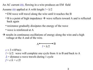
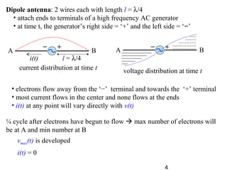
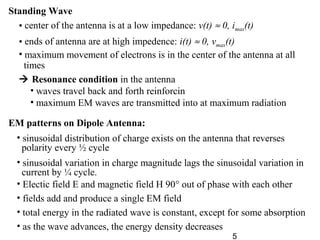
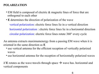
1
Key Points
1. Principals of EM Radiation
2. Introduction to Propagation & Antennas
3. Antenna Characterization
2
1. Principals of Radiated electromagentic (EM) fields
two laws (from Maxwell Equation)
1. A Moving Electric Field Creates a Magnetic (H) field
2. A Moving Magnetic Field Creates an Electric (E) field
3
c ≈ 3 ×10⁸
m/s
l = λ/2: wave will complete one cycle from A to B and back to A
λ = distance a wave travels during 1 cycle
f = c/λ = c/2l
l = λ/2
A B
Assume i(t) applied at A with length l = λ/2
• EM wave will travel along the wire until it reaches the B
• B is a point of high impedence  wave reflects toward A and is reflected
back again
• resistance gradually dissipates the energy of the wave
• wave is reinforced at A
 results in continuous oscillations of energy along the wire and a high
voltage at the A end of the wire.
An AC current i(t), flowing in a wire produces an EM field
4
Dipole antenna: 2 wires each with length l = λ/4
• attach ends to terminals of a high frequency AC generator
• at time t, the generator’s right side = ‘+’ and the left side = ‘−’
• electrons flow away from the ‘−’ terminal and towards the ‘+’ terminal
• most current flows in the center and none flows at the ends
• i(t) at any point will vary directly with v(t)
current distribution at time t
− +
i(t) l = λ/4
A B
− +
++++
+++++++
+++++++++++
+++++++++++++++
+++++++++++++++
-----
-----------
----------------
--------------------
------------------------
voltage distribution at time t
A B
¼ cycle after electrons have begun to flow  max number of electrons will
be at A and min number at B
vmax(t) is developed
i(t) = 0
5
EM patterns on Dipole Antenna:
• sinusoidal distribution of charge exists on the antenna that reverses
polarity every ½ cycle
• sinusoidal variation in charge magnitude lags the sinusoidal variation in
current by ¼ cycle.
• Electic field E and magnetic field H 90° out of phase with each other
• fields add and produce a single EM field
• total energy in the radiated wave is constant, except for some absorption
• as the wave advances, the energy density decreases
Standing Wave
• center of the antenna is at a low impedance: v(t) ≈ 0, imax(t)
• ends of antenna are at high impedence: i(t) ≈ 0, vmax(t)
• maximum movement of electrons is in the center of the antenna at all
times
 Resonance condition in the antenna
• waves travel back and forth reinforcin
• maximum EM waves are transmitted into at maximum radiation
6
POLARIZATION
• EM field is composed of electric & magnetic lines of force that are
orthogonal to each other
• E determines the direction of polarization of the wave
vertical polarization: electric force lines lie in a vertical direction
horizontal polarization : electric force lines lie in a horizontal direction
circular polarization: electric force lines rotate 360° every cycle
An antenna extracts maximumenergy from a passing EM wave when it is
oriented in the same direction as E
• use vertical antenna for the efficient reception of vertically polarized
waves
• use horizontal antenna for the reception of horizontally polarized waves
if E rotates as the wave travels through space  wave has. horizontal and
vertical components
7
Ground wave transmissions missions at lower frequencies use vertical
polarization
• horizontal polarization E force lines are parallel to and touch the earth.
earth acts as a fairly good conductor at low frequencies  shorts out
• vertical electric lines of force are bothered very little by the earth.
8
Types of antennas
• simple antennas: dipole, long wire
• complex antennas: additional components to
shape radiated field
provide high gain for long distances or weak signal reception
size ≈ frequency of operation
• combinations of identical antennas
phased arrays electrically shape and steer antenna
2. Introduction to Antennas and Propagation
transmit antenna: radiate maximum energy into surroundings
receive antenna: capture maximum energy from surrounding
• radiating transmission line is technically an antenna
• good transmission line = poor antenna
9
Major Difference Between Antennas And Transmission Lines
• transmission line uses conductor to carry voltage & current
• radio signal travels through air (insulator)
• antennas are transducers
- convert voltage & current into electric & magnetic field
- bridges transmission line & air
- similar to speaker/microphone with acoustic energy
Transmission Line
• voltage & current variations  produce EM field around conductor
• EM field expands & contracts at same frequency as variations
• EM field contractions return energy to the source (conductor)
• Nearly all the energy in the transmission line remains in the system
10
Antenna
• Designed to Prevent most of the Energy from returning to Conductor
• Specific Dimensions & EM wavelengths cause field to radiate
several λ before the Cycle Reversal
- Cycle Reversal - Field Collapses  Energy returns to Conductor
- Produces 3-Dimensional EM field
- Electric Field ⊥ Magnetic Field
- Wave Energy Propagation ⊥ Electric Field & Magnetic Field
11
transmit & receive antennas
theoretically are the same (e.g. radiation fields, antenna gain)
practical implementation issue:
transmit antenna handles high power signal (W-MW)
- large conductors & high power connectors,
receive antenna handles low power signal (mW-uW)
Antenna Performance depends heavily on
• Channel Characteristics: obstacles, distances temperature,…
• Signal Frequency
• Antenna Dimensions
12
Propagation Modes – five types
(1) Ground or Surface wave: follow earths contour
• affected by natural and man-made terrain
• salt water forms low loss path
• several hundred mile range
• 2-3 MHz signal
(2) Space Wave
• Line of Sight (LOS) wave
• Ground Diffraction allows for greater distance
• Approximate Maximum Distance, D in miles is
(antenna height in ft)
• No Strict Signal Frequency Limitations
rxtx hh 22 +D =
hrx
htx
13
(3) Sky Waves
ionosphere
transmitted
wave
reflected
wave
refracted
wave
skip distance
• reflected off ionosphere (20-250 miles high)
• large ranges possible with single hop or multi-hop
• transmit angle affects distance, coverage, refracted energy
14
Ionosphere
• is a layer of partially ionized gasses below troposphere
- ionization caused by ultra-violet radiation from the sun
- affected by: available sunlight, season, weather, terrain
- free ions & electrons reflect radiated energy
• consists of several ionized layers with varying ion density
- each layer has a central region of dense ionization
Layer altitude
(miles)
Frequency
Range
Availability
D 20-25 several MHz day only
E 55-90 20MHz day, partially
at night
F1 90-140 30MHz 24 hours
F2 200-250 30MHz 24 hours
F1 & F2 separate during daylight, merge at night
15
Usable Frequency and Angles
Critical Frequency: frequency that won’t reflect vertical transmission
- critical frequency is relative to each layer of ionosphere
- as frequency increases  eventually signal will not reflect
Maximum Usable Frequency (MUF): highest frequency useful for
reflected transmissions
- absorption by ionosphere decreases at higher frequencies
- absorption of signal energy = signal loss
- best results when MUF is used
Frequency Trade-Off
• high frequency signals eventually will not reflect back to ground
• lower frequency signals are attenuated more in the ionosphere
16
angle of radiation: transmitted energy relative to surface tangent
- smaller angle requires less ionospheric refraction to return to earth
- too large an angle results in no reflection
- 3o
-60o
are common angles
critical angle: maximum angle of radiation that will reflect energy
to earth
Determination of minimum skip distance:
- critical angle - small critical angle  long skip distance
- height of ionosphere - higher layers give longer skip distances
for a fixed angle
multipath: signal takes different paths to the destination
angle of radiation
ionosphere
Critical Angle
17
(4) Satellite Waves
Designed to pass through ionosphere into space
• uplink (ground to space)
• down link (space to ground)
• LOS link
Frequencies >> critical frequency
• penetrates ionosphere without reflection
• high frequencies provide bandwidth
Geosynchronous orbit ≈ 23k miles (synchronized with earth’s orbit)
• long distances  result in high path loss
• EM energy disperses over distances
• intensely focused beam improves efficiency
18
total loss = Gt + Gr – path loss (dB)
Free Space Path Loss equation used to determine signal levels
over distance
G = antenna gain: projection of energy in specific direction
• can magnify transmit power
• increase effective signal level at receiver
2
4






=
c
fd
P
P
r
t π






c
fdπ4
log20 10 (dB)
19
(5) radar: requires
• high gain antenna
• sensitive low noise receiver
• requires reflected signal from object – distances are doubled
• only small fraction of transmitted signal reflects back
20
3. Antenna Characterization
antennas generate EM field pattern
• not always possible to model mathematically
• difficult to account for obstacles
• antennas are studied in EM isolated rooms to extract key
performance characteristics
absolute value of signal intensity varies for given antenna design
- at the transmitter this is related to power applied at transmitter
- at the receiver this is related to power in surrounding space
antenna design & relative signal intensity determines relative field
pattern
21
forward gain = 10dB
backward gain = 7dB
+10dB
+7dB
+ 4dB
0o
270o
180o
90o
Polar Plot of relative signal strength of radiated field
• shows how field strength is shaped
• generally 0o
aligned with major physical axis of antenna
• most plots are relative scale (dB)
- maximum signal strength location is 0 dB reference
- closer to center represents weaker signals
22
radiated field shaping ≈ lens & visible light
• application determines required direction & focus of signal
• antenna characteristics
(i) radiation field pattern
(ii) gain
(iii) lobes, beamwidth, nulls
(iv) directivity
far-field measurements measured many wavelengths away from
antenna
near-field measurement involves complex interactions of decaying
electrical and magnetic fields - many details of antenna construction
(i) antenna field pattern = general shape of signal intensity in far-field
23
Measuring Antenna Field Pattern
field strength meter used to measure field pattern
• indicates amplitude of received signal
• calibrated to receiving antenna
• relationship between meter and receive antenna known
measured strength in uV/meter
received power is in uW/meter
• directly indicates EM field strength
24
0o
270o
180o
90o
Determination of overall Antenna Field Pattern
form Radiation Polar Plot Pattern
• use nominal field strength value (e.g. 100uV/m)
• measure points for 360o
around antenna
• record distance & angle from antenna
• connect points of equal field strength
100 uV/m
practically
• distance between meter & antenna kept constant
• antenna is rotated
• plot of field strength versus angle is made
25
Why Shape the Antenna Field Pattern ?
• transmit antennas: produce higher effective power in direction of
intended receiver
• receive antennas: concentrate energy collecting ability in
direction of transmitter
- reduced noise levels - receiver only picks up intended signal
• avoid unwanted receivers (multiple access interference = MAI):
- security
- multi-access systems
• locate target direction & distance – e.g. radar
not always necessary to shape field pattern, standard broadcast is
often omnidirectional - 360o
26
Gain is Measured Specific to a Reference Antenna
• isotropic antenna often used - gain over isotropic
- isotropic antenna – radiates power ideally in all directions
- gain measured in dBi
- test antenna’s field strength relative to reference isotropic antenna
- at same power, distance, and angle
- isotropic antenna cannot be practically realized
• ½ wave dipole often used as reference antenna
- easy to build
- simple field pattern
(ii) Antenna Gain
27
Antenna Gain ≠ Amplifier Gain
• antenna power output = power input – transmission line loss
• antenna shapes radiated field pattern
• power measured at a point is greater/less than that using
reference antenna
• total power output doesn’t increase
• power output in given direction increases/decreases relative to
reference antenna
e.g.
a lamp is similar to an isotropic antenna
a lens is similar to a directional antenna
- provides a gain/loss of visible light in a specific direction
- doesn’t change actual power radiated by lamp
28
Rotational Antennas can vary direction of antenna gain
Directional Antennas focus antenna gain in primary direction
• transmit antenna with 6dB gain in specific direction over isotropic
antenna  4× transmit power in that direction
• receive antenna with 3dB gain is some direction receives 2× as
much power than reference antenna
Antenna Gain
often a cost effective means to
(i) increase effective transmit power
(ii) effectively improve receiver sensitivity
may be only technically viable means
• more power may not be available (batteries)
• front end noise determines maximum receiver sensitivity
29
(iii) Beamwidth, Lobes & Nulls
Lobe: area of high signal strength
- main lobe
- secondary lobes
Nulls: area of very low signal strength
Beamwidth: total angle where relative signal power is 3dB
below peak value of main lobe
- can range from 1o
to 360o
Beamwidth & Lobes indicate sharpness of pattern focus
0o
270o
180o
90o
beam
width
null
30
Center Frequency = optimum operating frequency
Antenna Bandwidth ≡ -3dB points of antenna performance
Bandwidth Ratio: Bandwidth/Center Frequency
e.g. fc = 100MHz with 10MHz bandwidth
- radiated power at 95MHz & 105MHz = ½ radiated power at fc
- bandwidth ratio = 10/100 = 10%
31
Main Trade-offs for Antenna Design
• directivity & beam width
• acceptable lobes
• maximum gain
• bandwidth
• radiation angle
Bandwidth Issues
High Bandwidth Antennas tend to have less gain than
narrowband antennas
Narrowband Receive Antenna reduces interference from adjacent
signals & reduce received noise power
Antenna Design Basics
Antenna Dimensions
• operating frequencies determine physical size of antenna elements
• design often uses λ as a variable (e.g. 1.5 λ length, 0.25 λ spacing)
32
Testing & Adjusting Transmitter  use antenna’s electrical load
• Testing required for
- proper modulation
- amplifier operation
- frequency accuracy
• using actual antenna may cause significant interference
• dummy antenna used for transmitter design (not antenna design)
- same impedance & electrical characteristics
- dissipates energy vs radiate energy
- isolates antenna from problem of testing transmitter
33
Testing Receiver
• test & adjust receiver and transmission line without antenna
• use single known signal from RF generator
• follow on test with several signals present
• verify receiver operation first  then connect antenna to
verify antenna operation
Polarization
• EM field has specific orientation of E-field & M field
• Polarization Direction determined by antenna & physical orientation
• Classification of E-field polarization
- horizontal polarization : E-field parallel to horizon
- vertical polarization: E-field vertical to horizon
- circular polarization: constantly rotating
34
Transmit & Receive Antenna must have same Polarization for
maximum signal energy induction
• if polarizations aren’t same  E-field of radiated signal will try to
induce E-field into wire ⊥ to correct orientation
- theoretically no induced voltage
- practically – small amount of induced voltage
Circular Polarization
• compatible with any polarization field from horizontal to vertical
• maximum gain is 3dB less than correctly oriented horizontal or
vertically polarized antenna
35
Antenna Fundamentals
Dipole Antennas (Hertz): simple, old, widely used
- root of many advance antennas
• consists of 2 spread conductors of 2 wire transmission lines
• each conductor is ¼ λ in length
• total span = ½ λ + small center gap
Distinct voltage & current patterns
driven by transmission line at midpoint
• i = 0 at end, maximum at midpoint
• v = 0 at midpoint, ±vmax at ends
• purely resistive impedance = 73Ω
• easily matched to many transmission lines
gap
¼ λ¼ λ
½ λ
Transmission
Line
+v
-v
i
High Impedance 2k-3kΩ
Low Impedance 73Ω
36
E-field (E) & M-field (B) used to determine radiation pattern
• E goes through antenna ends & spreads out in increasing loops
• B is a series of concentric circles centered at midpoint gap
E B
37
Azimuth Pattern
Elevation Pattern
Polar Radiation Pattern
3-dimensional field pattern is donut shaped
antenna is shaft through donut center
radiation pattern determined by taking slice of donut
- if antenna is horizontal  slice reveals figure 8
- maximum radiation is broadside to antenna’s arms
38
½λ dipole performance – isotropic reference antenna
• in free space  beamwidth = 78o
• maximum gain = 2.1dB
• dipole often used as reference antenna
- feed same signal power through ½ λ dipole & test antenna
- compare field strength in all directions
Actual Construction
(i) propagation velocity in wire < propagation velocity in air
(ii) fields have ‘fringe effects’ at end of antenna arms
- affected by capacitance of antenna elements
1st
estimate: make real length 5% less than ideal - otherwise
introduce reactive parameter
Useful Bandwidth: 5%-15% of fc
• major factor for determining bandwidth is diameter of conductor
• smaller diameter  narrow bandwidth
39
Multi-Band Dipole Antennas
Transmission
Line
λ1/4C
L
C
L
λ1/4
λ2/4λ2/4
use 1 antenna  support several widely separated frequency bands
e.g. HAM Radio - 3.75MHz-29MHz
Traps: L,C elements inserted into dipole arms
• arms appear to have different lengths at different frequencies
• traps must be suitable for outdoor use
• 2ndry
affects of trap impact effective dipole arm length-adjustable
• not useful over 30MHz
40
Transmit Receive Switches
• allows use of single antenna for transmit & receive
• alternately connects antenna to transmitter & receiver
• high transmit power must be isolated from high gain receiver
• isolation measured in dB
e.g. 100dB isolation 10W transmit signal ≈ 10nW receive signal
41
Elementary Antennas
low cost – flexible solutions
Long Wire Antenna
• effective wideband antenna
• length l = several wavelengths
- used for signals with 0.1l < λ < 0.5l
- frequency span = 5:1
• drawback for band limited systems - unavoidable interference
• near end driven by ungrounded transmitter output
• far end terminated by resistor
- typically several hundred Ω
- impedance matched to antenna Z0
• transmitter electrical circuit ground connected to earth
Antenna
Transmission
Line
earth ground
R=Z0
42
practically - long wire is a lossy transmission line
- terminating resistor prevent standing waves
Polar radiation pattern
• 2 main lobes
- on either side of antenna
- pointed towards antenna termination
• smaller lobes on each side of antenna – pointing forward & back
• radiation angle 45o
(depending on height)  useful for sky waves
angular radiation pattern
horizon
feed
polar ration pattern
43
poor efficiency:
transmit power
- 50% of transmit power radiated
- 50% dissapated in termination resistor
receive power
- 50% captured EM energy converted to signal for reciever
- 50% absorbed by terminating resistor
44
Folded Dipole Antenna
- basic ½λ dipole folded to form complete circuit
- core to many advanced antennas
- mechanically more rugged than dipole
- 10% more bandwidth than dipole
- input impedance ≈ 292 Ω
- close match to std 300Ω twin lead wire transmission line
- use of different diameter upper & lower arms  allows
variable impedance
λ/2
45
Loop & Patch Antenna – wire bent into loops
Patch Antenna: rectangular conducting area with || ground plane
Area A
N-turns
V = maximum voltage induced in receiver by EM field
B = magnetic field strength flux of EM field
A = area of loop
N = number of turns
f = signal frequency
k = physical proportionality factor
V = k(2πf)BAN
Antenna
Plane
46
• Loop & Patch Antennas are easy to embed in a product (e.g. pager)
• Broadband antenna - 500k-1600k Hz bandwidth
• Not as efficient as larger antennas
Radiation Pattern
• maximum ⊥ to center axis through loop
• very low broadside to the loop
• useful for direction finding
- rotate loop until signal null (minimum) observed
- transmitter is on either side of loop
- intersection with 2nd
reading pinpoints transmitter
47
552.14 dB
Dipole
3600 dBIsotropic
Beamwidth
-3 dB
Gain (over
isotropic)
ShapeName Radiation Pattern
20
30
50
200
25
14.7 dB
10.1 dB
-0.86 dB
3.14 dB
7.14 dB
Parabolic
Dipole
Helical
Turnstile
Full Wave
Loop
Yagi
Biconical
Horn
1515 dBHorn
360x20014 dB

3 basic antenas1

  • 1.
    1 Key Points 1. Principalsof EM Radiation 2. Introduction to Propagation & Antennas 3. Antenna Characterization
  • 2.
    2 1. Principals ofRadiated electromagentic (EM) fields two laws (from Maxwell Equation) 1. A Moving Electric Field Creates a Magnetic (H) field 2. A Moving Magnetic Field Creates an Electric (E) field
  • 3.
    3 c ≈ 3×10⁸ m/s l = λ/2: wave will complete one cycle from A to B and back to A λ = distance a wave travels during 1 cycle f = c/λ = c/2l l = λ/2 A B Assume i(t) applied at A with length l = λ/2 • EM wave will travel along the wire until it reaches the B • B is a point of high impedence  wave reflects toward A and is reflected back again • resistance gradually dissipates the energy of the wave • wave is reinforced at A  results in continuous oscillations of energy along the wire and a high voltage at the A end of the wire. An AC current i(t), flowing in a wire produces an EM field
  • 4.
    4 Dipole antenna: 2wires each with length l = λ/4 • attach ends to terminals of a high frequency AC generator • at time t, the generator’s right side = ‘+’ and the left side = ‘−’ • electrons flow away from the ‘−’ terminal and towards the ‘+’ terminal • most current flows in the center and none flows at the ends • i(t) at any point will vary directly with v(t) current distribution at time t − + i(t) l = λ/4 A B − + ++++ +++++++ +++++++++++ +++++++++++++++ +++++++++++++++ ----- ----------- ---------------- -------------------- ------------------------ voltage distribution at time t A B ¼ cycle after electrons have begun to flow  max number of electrons will be at A and min number at B vmax(t) is developed i(t) = 0
  • 5.
    5 EM patterns onDipole Antenna: • sinusoidal distribution of charge exists on the antenna that reverses polarity every ½ cycle • sinusoidal variation in charge magnitude lags the sinusoidal variation in current by ¼ cycle. • Electic field E and magnetic field H 90° out of phase with each other • fields add and produce a single EM field • total energy in the radiated wave is constant, except for some absorption • as the wave advances, the energy density decreases Standing Wave • center of the antenna is at a low impedance: v(t) ≈ 0, imax(t) • ends of antenna are at high impedence: i(t) ≈ 0, vmax(t) • maximum movement of electrons is in the center of the antenna at all times  Resonance condition in the antenna • waves travel back and forth reinforcin • maximum EM waves are transmitted into at maximum radiation
  • 6.
    6 POLARIZATION • EM fieldis composed of electric & magnetic lines of force that are orthogonal to each other • E determines the direction of polarization of the wave vertical polarization: electric force lines lie in a vertical direction horizontal polarization : electric force lines lie in a horizontal direction circular polarization: electric force lines rotate 360° every cycle An antenna extracts maximumenergy from a passing EM wave when it is oriented in the same direction as E • use vertical antenna for the efficient reception of vertically polarized waves • use horizontal antenna for the reception of horizontally polarized waves if E rotates as the wave travels through space  wave has. horizontal and vertical components
  • 7.
    7 Ground wave transmissionsmissions at lower frequencies use vertical polarization • horizontal polarization E force lines are parallel to and touch the earth. earth acts as a fairly good conductor at low frequencies  shorts out • vertical electric lines of force are bothered very little by the earth.
  • 8.
    8 Types of antennas •simple antennas: dipole, long wire • complex antennas: additional components to shape radiated field provide high gain for long distances or weak signal reception size ≈ frequency of operation • combinations of identical antennas phased arrays electrically shape and steer antenna 2. Introduction to Antennas and Propagation transmit antenna: radiate maximum energy into surroundings receive antenna: capture maximum energy from surrounding • radiating transmission line is technically an antenna • good transmission line = poor antenna
  • 9.
    9 Major Difference BetweenAntennas And Transmission Lines • transmission line uses conductor to carry voltage & current • radio signal travels through air (insulator) • antennas are transducers - convert voltage & current into electric & magnetic field - bridges transmission line & air - similar to speaker/microphone with acoustic energy Transmission Line • voltage & current variations  produce EM field around conductor • EM field expands & contracts at same frequency as variations • EM field contractions return energy to the source (conductor) • Nearly all the energy in the transmission line remains in the system
  • 10.
    10 Antenna • Designed toPrevent most of the Energy from returning to Conductor • Specific Dimensions & EM wavelengths cause field to radiate several λ before the Cycle Reversal - Cycle Reversal - Field Collapses  Energy returns to Conductor - Produces 3-Dimensional EM field - Electric Field ⊥ Magnetic Field - Wave Energy Propagation ⊥ Electric Field & Magnetic Field
  • 11.
    11 transmit & receiveantennas theoretically are the same (e.g. radiation fields, antenna gain) practical implementation issue: transmit antenna handles high power signal (W-MW) - large conductors & high power connectors, receive antenna handles low power signal (mW-uW) Antenna Performance depends heavily on • Channel Characteristics: obstacles, distances temperature,… • Signal Frequency • Antenna Dimensions
  • 12.
    12 Propagation Modes –five types (1) Ground or Surface wave: follow earths contour • affected by natural and man-made terrain • salt water forms low loss path • several hundred mile range • 2-3 MHz signal (2) Space Wave • Line of Sight (LOS) wave • Ground Diffraction allows for greater distance • Approximate Maximum Distance, D in miles is (antenna height in ft) • No Strict Signal Frequency Limitations rxtx hh 22 +D = hrx htx
  • 13.
    13 (3) Sky Waves ionosphere transmitted wave reflected wave refracted wave skipdistance • reflected off ionosphere (20-250 miles high) • large ranges possible with single hop or multi-hop • transmit angle affects distance, coverage, refracted energy
  • 14.
    14 Ionosphere • is alayer of partially ionized gasses below troposphere - ionization caused by ultra-violet radiation from the sun - affected by: available sunlight, season, weather, terrain - free ions & electrons reflect radiated energy • consists of several ionized layers with varying ion density - each layer has a central region of dense ionization Layer altitude (miles) Frequency Range Availability D 20-25 several MHz day only E 55-90 20MHz day, partially at night F1 90-140 30MHz 24 hours F2 200-250 30MHz 24 hours F1 & F2 separate during daylight, merge at night
  • 15.
    15 Usable Frequency andAngles Critical Frequency: frequency that won’t reflect vertical transmission - critical frequency is relative to each layer of ionosphere - as frequency increases  eventually signal will not reflect Maximum Usable Frequency (MUF): highest frequency useful for reflected transmissions - absorption by ionosphere decreases at higher frequencies - absorption of signal energy = signal loss - best results when MUF is used Frequency Trade-Off • high frequency signals eventually will not reflect back to ground • lower frequency signals are attenuated more in the ionosphere
  • 16.
    16 angle of radiation:transmitted energy relative to surface tangent - smaller angle requires less ionospheric refraction to return to earth - too large an angle results in no reflection - 3o -60o are common angles critical angle: maximum angle of radiation that will reflect energy to earth Determination of minimum skip distance: - critical angle - small critical angle  long skip distance - height of ionosphere - higher layers give longer skip distances for a fixed angle multipath: signal takes different paths to the destination angle of radiation ionosphere Critical Angle
  • 17.
    17 (4) Satellite Waves Designedto pass through ionosphere into space • uplink (ground to space) • down link (space to ground) • LOS link Frequencies >> critical frequency • penetrates ionosphere without reflection • high frequencies provide bandwidth Geosynchronous orbit ≈ 23k miles (synchronized with earth’s orbit) • long distances  result in high path loss • EM energy disperses over distances • intensely focused beam improves efficiency
  • 18.
    18 total loss =Gt + Gr – path loss (dB) Free Space Path Loss equation used to determine signal levels over distance G = antenna gain: projection of energy in specific direction • can magnify transmit power • increase effective signal level at receiver 2 4       = c fd P P r t π       c fdπ4 log20 10 (dB)
  • 19.
    19 (5) radar: requires •high gain antenna • sensitive low noise receiver • requires reflected signal from object – distances are doubled • only small fraction of transmitted signal reflects back
  • 20.
    20 3. Antenna Characterization antennasgenerate EM field pattern • not always possible to model mathematically • difficult to account for obstacles • antennas are studied in EM isolated rooms to extract key performance characteristics absolute value of signal intensity varies for given antenna design - at the transmitter this is related to power applied at transmitter - at the receiver this is related to power in surrounding space antenna design & relative signal intensity determines relative field pattern
  • 21.
    21 forward gain =10dB backward gain = 7dB +10dB +7dB + 4dB 0o 270o 180o 90o Polar Plot of relative signal strength of radiated field • shows how field strength is shaped • generally 0o aligned with major physical axis of antenna • most plots are relative scale (dB) - maximum signal strength location is 0 dB reference - closer to center represents weaker signals
  • 22.
    22 radiated field shaping≈ lens & visible light • application determines required direction & focus of signal • antenna characteristics (i) radiation field pattern (ii) gain (iii) lobes, beamwidth, nulls (iv) directivity far-field measurements measured many wavelengths away from antenna near-field measurement involves complex interactions of decaying electrical and magnetic fields - many details of antenna construction (i) antenna field pattern = general shape of signal intensity in far-field
  • 23.
    23 Measuring Antenna FieldPattern field strength meter used to measure field pattern • indicates amplitude of received signal • calibrated to receiving antenna • relationship between meter and receive antenna known measured strength in uV/meter received power is in uW/meter • directly indicates EM field strength
  • 24.
    24 0o 270o 180o 90o Determination of overallAntenna Field Pattern form Radiation Polar Plot Pattern • use nominal field strength value (e.g. 100uV/m) • measure points for 360o around antenna • record distance & angle from antenna • connect points of equal field strength 100 uV/m practically • distance between meter & antenna kept constant • antenna is rotated • plot of field strength versus angle is made
  • 25.
    25 Why Shape theAntenna Field Pattern ? • transmit antennas: produce higher effective power in direction of intended receiver • receive antennas: concentrate energy collecting ability in direction of transmitter - reduced noise levels - receiver only picks up intended signal • avoid unwanted receivers (multiple access interference = MAI): - security - multi-access systems • locate target direction & distance – e.g. radar not always necessary to shape field pattern, standard broadcast is often omnidirectional - 360o
  • 26.
    26 Gain is MeasuredSpecific to a Reference Antenna • isotropic antenna often used - gain over isotropic - isotropic antenna – radiates power ideally in all directions - gain measured in dBi - test antenna’s field strength relative to reference isotropic antenna - at same power, distance, and angle - isotropic antenna cannot be practically realized • ½ wave dipole often used as reference antenna - easy to build - simple field pattern (ii) Antenna Gain
  • 27.
    27 Antenna Gain ≠Amplifier Gain • antenna power output = power input – transmission line loss • antenna shapes radiated field pattern • power measured at a point is greater/less than that using reference antenna • total power output doesn’t increase • power output in given direction increases/decreases relative to reference antenna e.g. a lamp is similar to an isotropic antenna a lens is similar to a directional antenna - provides a gain/loss of visible light in a specific direction - doesn’t change actual power radiated by lamp
  • 28.
    28 Rotational Antennas canvary direction of antenna gain Directional Antennas focus antenna gain in primary direction • transmit antenna with 6dB gain in specific direction over isotropic antenna  4× transmit power in that direction • receive antenna with 3dB gain is some direction receives 2× as much power than reference antenna Antenna Gain often a cost effective means to (i) increase effective transmit power (ii) effectively improve receiver sensitivity may be only technically viable means • more power may not be available (batteries) • front end noise determines maximum receiver sensitivity
  • 29.
    29 (iii) Beamwidth, Lobes& Nulls Lobe: area of high signal strength - main lobe - secondary lobes Nulls: area of very low signal strength Beamwidth: total angle where relative signal power is 3dB below peak value of main lobe - can range from 1o to 360o Beamwidth & Lobes indicate sharpness of pattern focus 0o 270o 180o 90o beam width null
  • 30.
    30 Center Frequency =optimum operating frequency Antenna Bandwidth ≡ -3dB points of antenna performance Bandwidth Ratio: Bandwidth/Center Frequency e.g. fc = 100MHz with 10MHz bandwidth - radiated power at 95MHz & 105MHz = ½ radiated power at fc - bandwidth ratio = 10/100 = 10%
  • 31.
    31 Main Trade-offs forAntenna Design • directivity & beam width • acceptable lobes • maximum gain • bandwidth • radiation angle Bandwidth Issues High Bandwidth Antennas tend to have less gain than narrowband antennas Narrowband Receive Antenna reduces interference from adjacent signals & reduce received noise power Antenna Design Basics Antenna Dimensions • operating frequencies determine physical size of antenna elements • design often uses λ as a variable (e.g. 1.5 λ length, 0.25 λ spacing)
  • 32.
    32 Testing & AdjustingTransmitter  use antenna’s electrical load • Testing required for - proper modulation - amplifier operation - frequency accuracy • using actual antenna may cause significant interference • dummy antenna used for transmitter design (not antenna design) - same impedance & electrical characteristics - dissipates energy vs radiate energy - isolates antenna from problem of testing transmitter
  • 33.
    33 Testing Receiver • test& adjust receiver and transmission line without antenna • use single known signal from RF generator • follow on test with several signals present • verify receiver operation first  then connect antenna to verify antenna operation Polarization • EM field has specific orientation of E-field & M field • Polarization Direction determined by antenna & physical orientation • Classification of E-field polarization - horizontal polarization : E-field parallel to horizon - vertical polarization: E-field vertical to horizon - circular polarization: constantly rotating
  • 34.
    34 Transmit & ReceiveAntenna must have same Polarization for maximum signal energy induction • if polarizations aren’t same  E-field of radiated signal will try to induce E-field into wire ⊥ to correct orientation - theoretically no induced voltage - practically – small amount of induced voltage Circular Polarization • compatible with any polarization field from horizontal to vertical • maximum gain is 3dB less than correctly oriented horizontal or vertically polarized antenna
  • 35.
    35 Antenna Fundamentals Dipole Antennas(Hertz): simple, old, widely used - root of many advance antennas • consists of 2 spread conductors of 2 wire transmission lines • each conductor is ¼ λ in length • total span = ½ λ + small center gap Distinct voltage & current patterns driven by transmission line at midpoint • i = 0 at end, maximum at midpoint • v = 0 at midpoint, ±vmax at ends • purely resistive impedance = 73Ω • easily matched to many transmission lines gap ¼ λ¼ λ ½ λ Transmission Line +v -v i High Impedance 2k-3kΩ Low Impedance 73Ω
  • 36.
    36 E-field (E) &M-field (B) used to determine radiation pattern • E goes through antenna ends & spreads out in increasing loops • B is a series of concentric circles centered at midpoint gap E B
  • 37.
    37 Azimuth Pattern Elevation Pattern PolarRadiation Pattern 3-dimensional field pattern is donut shaped antenna is shaft through donut center radiation pattern determined by taking slice of donut - if antenna is horizontal  slice reveals figure 8 - maximum radiation is broadside to antenna’s arms
  • 38.
    38 ½λ dipole performance– isotropic reference antenna • in free space  beamwidth = 78o • maximum gain = 2.1dB • dipole often used as reference antenna - feed same signal power through ½ λ dipole & test antenna - compare field strength in all directions Actual Construction (i) propagation velocity in wire < propagation velocity in air (ii) fields have ‘fringe effects’ at end of antenna arms - affected by capacitance of antenna elements 1st estimate: make real length 5% less than ideal - otherwise introduce reactive parameter Useful Bandwidth: 5%-15% of fc • major factor for determining bandwidth is diameter of conductor • smaller diameter  narrow bandwidth
  • 39.
    39 Multi-Band Dipole Antennas Transmission Line λ1/4C L C L λ1/4 λ2/4λ2/4 use1 antenna  support several widely separated frequency bands e.g. HAM Radio - 3.75MHz-29MHz Traps: L,C elements inserted into dipole arms • arms appear to have different lengths at different frequencies • traps must be suitable for outdoor use • 2ndry affects of trap impact effective dipole arm length-adjustable • not useful over 30MHz
  • 40.
    40 Transmit Receive Switches •allows use of single antenna for transmit & receive • alternately connects antenna to transmitter & receiver • high transmit power must be isolated from high gain receiver • isolation measured in dB e.g. 100dB isolation 10W transmit signal ≈ 10nW receive signal
  • 41.
    41 Elementary Antennas low cost– flexible solutions Long Wire Antenna • effective wideband antenna • length l = several wavelengths - used for signals with 0.1l < λ < 0.5l - frequency span = 5:1 • drawback for band limited systems - unavoidable interference • near end driven by ungrounded transmitter output • far end terminated by resistor - typically several hundred Ω - impedance matched to antenna Z0 • transmitter electrical circuit ground connected to earth Antenna Transmission Line earth ground R=Z0
  • 42.
    42 practically - longwire is a lossy transmission line - terminating resistor prevent standing waves Polar radiation pattern • 2 main lobes - on either side of antenna - pointed towards antenna termination • smaller lobes on each side of antenna – pointing forward & back • radiation angle 45o (depending on height)  useful for sky waves angular radiation pattern horizon feed polar ration pattern
  • 43.
    43 poor efficiency: transmit power -50% of transmit power radiated - 50% dissapated in termination resistor receive power - 50% captured EM energy converted to signal for reciever - 50% absorbed by terminating resistor
  • 44.
    44 Folded Dipole Antenna -basic ½λ dipole folded to form complete circuit - core to many advanced antennas - mechanically more rugged than dipole - 10% more bandwidth than dipole - input impedance ≈ 292 Ω - close match to std 300Ω twin lead wire transmission line - use of different diameter upper & lower arms  allows variable impedance λ/2
  • 45.
    45 Loop & PatchAntenna – wire bent into loops Patch Antenna: rectangular conducting area with || ground plane Area A N-turns V = maximum voltage induced in receiver by EM field B = magnetic field strength flux of EM field A = area of loop N = number of turns f = signal frequency k = physical proportionality factor V = k(2πf)BAN Antenna Plane
  • 46.
    46 • Loop &Patch Antennas are easy to embed in a product (e.g. pager) • Broadband antenna - 500k-1600k Hz bandwidth • Not as efficient as larger antennas Radiation Pattern • maximum ⊥ to center axis through loop • very low broadside to the loop • useful for direction finding - rotate loop until signal null (minimum) observed - transmitter is on either side of loop - intersection with 2nd reading pinpoints transmitter
  • 47.
    47 552.14 dB Dipole 3600 dBIsotropic Beamwidth -3dB Gain (over isotropic) ShapeName Radiation Pattern 20 30 50 200 25 14.7 dB 10.1 dB -0.86 dB 3.14 dB 7.14 dB Parabolic Dipole Helical Turnstile Full Wave Loop Yagi Biconical Horn 1515 dBHorn 360x20014 dB