This document presents a new method for creating proxy models called Simulated Annealing Programming (SAP). SAP uses simulated annealing optimization on a tree structure to find the equation that best predicts outputs with minimum error. The authors apply SAP to create a model for predicting gas compressor torque based on fuel rate and speed. They find the SAP model is highly accurate, roughly independent of internal parameters, and has smaller overestimation/underestimation compared to other methods like polynomials and neural networks.

1. www.iiec2015.org
A New Proxy Model, Based On Meta heuristic
Algorithms For Estimating Gas Compressor Torque
Mohammad Reza Mahdiani Ramin Soltanmohamadi
Amir Kabir University of Technology (Tehran Polytechnic) Amir Kabir University of Technology (Tehran Polytechnic)
Tehran, Iran Tehran, Iran
mrmahdiani@aut.ac.ir raminsoltan999@yahoo.com
Ehsan Khamehchi Babak Azkayi
Amir Kabir University of Technology (Tehran Polytechnic) Amir Kabir University of Technology (Tehran Polytechnic)
Tehran, Iran Tehran, Iran
khamehchi@aut.ac.ir b.azkayi@yahoo.com
Abstract— there are various types of machine learning
methods or proxy models in literatures. But most of them
are not accurate enough, have a huge error in some points
and are aggressively dependent on their internal parameters
that causes different run of them leads to different models
with different prediction and accuracy. In this paper, an
attempt has been made to find a new artificial intelligence
method to create proxy models. In this method, simulated
annealing is applied on a tree structure to change its shape
to a form in which its corresponding equation has minimum
errors in predicting the outputs. Afterwards, in a case study
of predicting a compressor torque, this model has been
compared with most common artificial intelligence methods
such as polynomial of degree one and two and artificial
neural network. And finally its applicability has been
discussed. It is observed that the new model is highly
accurate, roughly independent of its internal parameters
and comparing with other methods its overestimation and
underestimation is small.
Keywords- Artificial Intelligence, Simulated Annealing,
artificial neural network, polynomial regression, spline
regression
I. INTRODUCTION
There are various cases in experimental science in which a
parameter needs to be calculated and usually it is a
function of some other parameters. The most accurate
method for finding its value is experiment or at least
simulation, but both are expensive and time consuming.
So finding a model that can predict the concerned
parameter using some other parameters is necessary. This
relationship which is called the proxy model calculates the
result rapidly and cheaply but a little less accurately than
an experimental one [1,2]. There are various methods for
creating proxy models. Here the most important of them
will be discussed.
In 1951, Box and Wilson [3,4] introduced response
surface methodology in which a n-degree polynomial
(usually second-degree) is fitted on the experimental
points. This method’s applicability is not good when the
number of input parameters increases. Another model is
splines which was introduced by Fridman in 1991 [5] and
is some kind of polynomials, works well in low degrees,
but becomes very complex at high degrees. After all,
Polynomial regression is not an accurate method [6].
Afterwards, the Kriging method was introduced by
Matron [7] in 1965. This method is less complex and
more accurate than previously introduced ones, but its
problem is having limited applicability and not being used
easily in different problems. In 1995, the artificial neural
network was introduced by Anderson [8]. This method
just needs to be trained and after that it can estimate the
results and be used easily in different problems [9,10].
However, it doesn’t give an explicit equation, different
runs of that have different models, and in some problems
their prediction is not very well [11], [12], [13]. As well as
in this year Bartels [14] introduced a spline modeling.
Spline divides data to some groups and then for each
group fits a curve. In 2004 Yang [15] presented a
geometric algorithm for conic spline curve fitting. He
used some examples to show the efficiency of his model.
In 2010 Flory [16] studied surface fitting and challenged
least square method which is a base for testing all
modeling methods. In 2014 Mitrut [17] studied the ways
of tuning proxy models. His tested his result in economic

2. www.iiec2015.org
problems. Also in this year Panjalizadeh [18] modified the
neural network to a dynamic response surface; he tested
his method in petroleum engineering. As seen there are
different methods for modeling in literature. But most of
them are not accurate or they don’t represent a simple
equation. Here using simulated annealing a model (which
we call simulated annealing programming, SAP) is
introduced which is accurate and represent a simple
equation.
II. BUILDING THE MODEL
In this paper, an attempt is made to find a proxy model
using the simulated annealing optimization method. For
this means, the tree representation has been used. This
representation is so flexible and can be used in different
fields of science and engineering such as identification of
steady state [19], kinetic orders [20] and differential
equations [21]. A tree representation can be seen in Fig. 1.
A tree stands for an equation. Here we want to find an
equation with the least error.
Simulated annealing is based on slow cooling and creation
of crystals. In this method, we have two functions of
temperature and free thermodynamic energy. Temperature
determines the chance of acceptance of bad solutions, and
free thermodynamic energy is in fact our objective
function [22]; in this algorithm first a possible solution is
supposed and its fitness is calculated, then using neighbor
concept it is modified. Afterward based on the fitness of
modified solution and the temperature, the new solution
may catch the position of previous solution. In usual
algorithms, the solution is a series of numbers, but here
we suppose that as a tree. By this definition, the algorithm
can be continued normally, while the only problem is the
neighbor. We need a new definition for neighbor which
can be applied in tree structure.
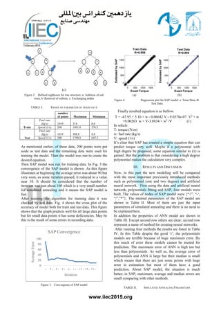
Neighbor
We suppose a tree as a crystal. For increasing the size of
the crystal in a non-deficient way some new molecule
should be added in suitable places and the molecules on a
bad position should be removed. Using this, three
methods are defined to optimize the size of the tree
structure.
1. Adding a sub tree: a sub tree is created randomly
and it is added to a random node in a tree. In this
method, the node that is common between the
tree and sub tree takes the value of the sub tree
(Fig. 2a).
2. Removing a sub tree: a node and its entire
connected branch are removed and a random
acceptable value is put in the place of the
removed node (Fig. 3b).
3. Exchanging nodes: Two nodes are selected
randomly and their place with all their connected
branches will be exchanged (Error! Reference
source not found. 2c).
In this study, the chance of occurrence of all the above
methods was equal. So, with this definition and
considering the trees as the state and energy as the average
error of the estimated value that the equation of the tree
causes, the modeling algorithm of this study be similar to
the normal simulated annealing.
Here before building the model, it’s necessary to explain a
little more about the used data and the problem.
Figure 1. A typicsl tree structure
A gas compressor is a part of machinery that increases the
pressure of gas by decreasing its volume. There are
different kinds of gas compressors that can work by
electricity or fuel, based on their usage. All of them have
an engine that creates torque and that torque cause the gas
to be pressurized.
Here the data of a fuel consuming compressor is gathered.
This data was donated by Professor Martin T. of Hagan of
Oklahoma State University [23]. These data gives the
torque of engine based on fuel rate and speed and that
contains 1199 points. The range of this data which used
for training and testing the model is shown in TABLE I.
(a)
(b)

3. www.iiec2015.org
(c)
Figure 2. Defined nighbours for tree structure; a: Addition of sub
trees, b: Removal of subtree, c: Exchanging nodes
TABLE I. RANGE OF PARAMETER OF TRAIN DATA
number
of points Maximum Minimum
Train
Fuel rate
(kg/s) 1019 314 0.6
Speed (1/s) 200 1801.8 576.2
Test
Fuel rate
(kg/s) 1019 308.8 0.8
Speed (1/s) 200 1799.8 647.3
As mentioned earlier, of these data, 200 points were put
aside as test data and the remaining data were used for
training the model. Then the model was run to create the
desired equation.
Then SAP model was run for training data. In Fig. 3 the
convergence of the SAP model is shown. As this figure
illustrates at beginning the average error was about 90 but
very soon, as some iteration passed, it reduced to a value
near 10. It should be considered that the number of
iteration was just about 160 which is a very small number
for simulated annealing and it means the SAP model is
fast.
After running the algorithm for training data it was
checked by test data. Fig. 4 shows the cross plot of the
accuracy of model both for train and test data. This figure
shows that the graph predicts well for all large data points
but for small data points it has some deficiencies. May be
this is the result of some errors in recording data.
Figure 3. Convergence of SAP model
(a) (b)
Figure 4. Regression plot for SAP model: a. Train Data, B.
Test Data
Finally resulted equation is as bellow:
T = -47.95 + 5.10 × w - 0.06642 V - 9.0378e-07 V2
× w
+0.00263 w × V-3.8834 × w2
/V (1)
In which:
T: torque (N.m)
w: fuel rate (kg/s)
V: speed (1/s)
It’s clear that SAP has created a simple equation that can
predict torque very well. Maybe if a polynomial with
high degree be proposed, some equation similar to (1) is
gained. But the problem is that considering a high degree
polynomial makes the calculation very complex.
III. RESULTS AND DISCUSSION
Now, in this part the new modeling will be compared
with the most important previously introduced methods
such as polynomial (one and two degree) and artificial
neural network. First using the data and artificial neural
network, polynomials fitting and SAP, four models were
built. The values of nodes of SAP model were {“+”, “-‘,
“/”,”*”}. The internal parameters of the SAP model are
shown in Table II. Most of them are just the input
parameters of simulated annealing and there is no need to
be explained here.
In addition the properties of ANN model are shown in
Table III. Except second row others are clear; second row
represent a name of method for creating neural networks.
After running four methods the results are listed in Table
IV. In this Table despite the good ‘r’, the polynomials
models are terrible because of huge maximum error. By
this much of error these models cannot be trusted for
prediction. The maximum error of ANN is high too but
less than polynomials. As well as, the average error of
polynomials and ANN is large but their median is small
which means that there are just some points with huge
error in estimation but most of them have a good
prediction. About SAP model, the situation is much
better; in SAP, maximum, average and median errors are
small comparing with other methods.
TABLE II. SIMULATED ANNEALING PARAMETERS
0
20
40
60
80
100
0 20 40 60 80 100 120 140 160
AverageError
Iteration
SAP Convergence
0 500 1000 1500
0
500
1000
1500
Exact Torque
EstimatedbySAP
Train Data
R=0.999
0 500 1000 1500
0
500
1000
1500
Exact Torque
EstimatedbySAP
Test Data
R=0.999

4. www.iiec2015.org
Parameter Value
Annealing Function Fast annealing
Re annealing interval 100
Temperature Update Function Exponential
Temperature Update Coefficient 0.96
Initial temperature 100
Stop Tolerance 1.00E-5
maximum tree depth 10
TABLE III. ARTIFICIAL NEURAL NETWORK PROPERTIES
Parameter Value
Data division Random
Training Levenberg-Marquart
Performance Mean Square Error
Stop tolerance 1.00E-05
TABLE IV. RESULT OF DIFFERENT ALGORITHMS ESTIMATIONS
Polynomia
l degree 1
Polynomia
l degree 2
Artificial
Neural
Network
SAP
mode
l
maximum
Error (%) 1689.33 1394.34 605.48 111
Average
Error (%) 30.45 31 14.82 9.4
Median
Error (%) 4.54 6.14 1.34 1.9
r 0.95 0.96 0.99 0.99
Figure 4 shows the regression of estimated point versus
exact values. In this figure all points are fitted wells, so
where are the huge errors of Table IV. Infect these huge
errors have happen in points near zero and thus small
deviation caused huge percent of errors. It can be inferred
that polynomials and ANN do not have a good estimation
in small values but SAP estimation is much better in both
small and large values.
Figure 5 shows the error distribution of different
algorithms. In all algorithms most of points have a small
error. In polynomial degree 1 small fraction of points have
an error of -2000% percent which is not ignorable at all,
polynomial degree 2 has overestimated by an 1500 %
error and artificial neural network which is much more
accurate than pervious methods have an error of 400%.
Again SAP model is better than other methods and its
error is just about 100%.
(a) (b)
(c) (d)
Figure 5. Regression of different inevstigated models: a: polynomial
of degree one, b: polynomial of degree two, c: artificial neural network,
d: SAP modeling of this paper
(a) (b)
(c) (d)
Figure 6. Error distribution of different investigated models; a:
polynomial of degree one, b: polynomial of degree two, c: artificial
neural network, d: SAP modeling of this paper
IV. CONCLUSION
1. The new SAP model can build the models with
high accuracy. And different runs of that results
the same model.
2. The estimation of the SAP model is near the
exact value and usually does not have the huge
underestimation and over estimations. Thus its
estimation is trustable.
3. After SAP model, artificial neural network and
after that polynomial has a good accuracy.
4. The model of this paper can be used in other
courses of science and engineering and for other
case studies than that of this paper.
0 500 1000 1500
0
500
1000
1500
Exact Torque
EstimatedTorque
Polynomial Degree 1
R=0.9735
0 500 1000 1500
0
500
1000
1500
Exact Torque
EstimatedTorque
Polynomial Degree 2
R=0.9779
0 500 1000 1500
0
500
1000
1500
Exact Torque
EstimatedTorque
Artificial Neural network
R=0.995
0 500 1000 1500
0
500
1000
1500
Exact Torque
EstidmatedTorque
SAP modeling
R=0.99
-2000 -1000 0 1000
0
50
100
150
200
Polynomial Degree 1
-500 0 500 1000 1500
0
50
100
150
200
Polynomial Degree 2
-1000 -500 0 500
0
50
100
150
200
Artificial Neural Network
-200 -100 0 100 200
0
20
40
60
80
100
120
Simulated Annealing Programming

5. www.iiec2015.org
REFERENCES
[1] D.R. Jones, "A taxonomy of global optimization methods based on
response surfaces," Journal of Global Optimization, vol. 21, pp.
345-383, 2001.
[2] SPE, and T. Graf, SPE, Schlumberger, and A. Al-Kinani, SPE,
Mining U. Leoben G. Zangl, "Proxy Modeling in Production
Optimization," in SPE Europec/EAGE Annual Conference and
Exhibition, Vienna, Austria, 2006.
[3] G. E. P. and Wilson, K.B. Box, "On the Experimental Attainment
of Optimum Conditions," Journal of the Royal Statistical Society,
vol. 13, no. 1, pp. 1-45, 1951.
[4] George E. P. Box, "Improving Almost Anything: Ideas and Essays,
Revised Edition," Wiley Series in Probability and Statistics, 1951.
[5] J.H. Friedman, "Multirative Adaptive regression Splines," Annalas
of Statistics, vol. 19, no. 1, 1991.
[6] Grace Wahba, "Spline Models for Observational Data," SAIM, vol.
59, p. 162, 1990.
[7] Christopher K.I. Williams, "Prediction with Gaussian processes:
From linear regression to linear prediction and beyond," Learning
in graphical models. MIT Press, pp. 599-612, 1998.
[8] J. A. Anderson, An Introduction to Neural Networks.: Cambridge,
MA: MIT Press., 1995.
[9] B. Yeten, A. Castellini, B. Guyaguler, and W.H. Chen, "A
Comparision Study on Experiment Design and responce Surface
Methodologies," in SPE Reservoir Simulation Symposium, Huston,
TX, 2005.
[10] J. Lencher and G. Zangl, "Treating Uncertanities in Reservoir
Prediction with Neural Networks," in SPE Europe/EAGE Annual
Conference, Madrid, Spain, 2005.
[11] Z. Zhao and J. Jian, "Attracting and quasi-invariant sets for BAM
neural networks of neutral-type with time-varying and infinite
distributed delays," Neurocomputing, vol. 140, pp. 265–272, 2014.
[12] Y. Gao et al., "Daylight perceptive lighting and data fusion with
artificial neutral network," Optik - International Journal for Light
and Electron Optics, vol. 125, no. 10, pp. 2405–2408, 2014.
[13] M. Ghaedi, A. Ansari, F. Bahari, A.M. Ghaedi, and A. Vafaei, "A
hybrid artificial neural network and particle swarm optimization
for prediction of removal of hazardous dye brilliant green from
aqueous solution using zinc sulfide nanoparticle loaded on
activated carbon," Spectrochimica Acta Part A: Molecular and
Biomolecular Spectroscopy, vol. 137, pp. 1004–1015, 2015.
[14] R.H. Bartels, J.C. Bartels, and B.A. Barsky, "an introduction to
splines for use in computer graphics and geometric modeling (the
morgan kaufmann series in computer graphics)," Engineering &
Trnsportation, 1995.
[15] X. Yang, "Curve fitting and fairing using conic splines,"
Computer-Aided Design, vol. 36, pp. 461–472, 2004.
[16] S. Flöry and M. Hofer, "Surface fitting and registration of point
clouds using approximations of the unsigned distance function,"
Computer Aided Geometric Design, vol. 27, pp. 60–77, 2010.
[17] C. Mitrut and M. Simionescu, "A Procedure for Selecting the Best
Proxy Variable Used in Predicting the Consumer Prices Index in
Romania," Procedia Economics and Finance, pp. 184-187, 2014.
[18] H. Panjalizadeh, N. Alizadeh, and H. Mashhadi , "A workflow for
risk analysis and optimization of steam flooding scenario using
static and dynamic proxy models," Journal of Petroleum Science
and Engineering, vol. 121, pp. 78–86, 2014.
[19] B. McKay, M. Willis, and G. Barton, "Steady-state modelling of
chemical process systems using genetic programming.," vol. 21,
pp. 981-986, 1997.
[20] H. Cao, J. Yu, L. Kang, and Y. Chen, "The kinetic evolutionary
modelling of complex systems of chemical reactions.," vol. 23, pp.
123-151, 1999.
[21] Eissa M. El-M. Shokir and Hazim N. Dmour, "Genetic
Programming (GP)-Based Model for the Viscosity of Pure and
Hydrocarbon Gas Mixtures," vol. 23, 2009.
[22] S. Kirkpatrick, C. D. Gelatt, and M. P. Vecchi, "Optimization by
Simulated Annealing," Science, vol. 220, pp. 671-680, 1983.
[23] T. Martin. (2014) Professor Martin T. of Hagan of Oklahoma State
University. [Online]. http://hagan.okstate.edu/
[24] M.J. Chen, Y.F. Hsu, and Y.C. Wu, "Modified penalty function
method for optimal social welfare of electric power supply chain
with transmission," International Journal of Electrical Power &
Energy Systems, vol. 57, pp. 90-96, 2014.
[25] M. Hovd and F. Stoican, "On the design of exact penalty functions
for mpc using mixed integer programming," Computers &
Chemical Engineering, pp. 104–113, 2014.
[26] A.F. Alkaya, V. Aksakalli, and C.E. Priebec, "A penalty search
algorithm for the obstacle neutralization problem," Computers &
Operations Research, vol. 53, pp. 165–175, 2015.
[27] H.L. Khoo, "Dynamic penalty function approach for ramp
metering with equity constraints," Journal of King Saud University
- Science, pp. 273–279, 2011.
[28] S.J. Lian, "Smoothing approximation to l1l1 exact penalty function
for inequality constrained optimization," Applied Mathematics and
Computation, pp. 3113–3121, 2012.
[29] C.H. Lin, "A rough penalty genetic algorithm for constrained
optimization," Information Sciences, pp. 119–137, 2013.
[30] M. Mahmudi and M.T. Sadeghi, "The optimization of continuous
gas lift pocess using an integrated compositional model," Journal
of Petroleum Science and Engineering, vol. 108, pp. 321-327,
2013.
[31] V.V.d. Melo and G. Iacca, "A modified covariance matrix
adaptation evolution strategy with adaptive penalty function and
Restart for constrained optimization," Expert Systems with
Applications, vol. 41, pp. 7077–7094, 2014.
[32] M. Mitchell (Author), An introduction to genetic algorithms
(complex adaptive systems.: A Bradford Book, 1998.
[33] R.L.U.d.F. Pinto and R.P.M. Ferreira, "An exact penalty function
based on the projection matrix," Applied Mathematics and
Computation, pp. 66–73, 2014.
[34] B. Srinivasan, L.T. Biegler, and D. Bonvin, "Tracking the
necessary conditions of optimality with changing set of active
constraints using a barrier-penalty function," Computers &
Chemical Engineering, pp. 572–579, 2008.
[35] G. Takacs, Gas lift manual.: PennWell, 2005.