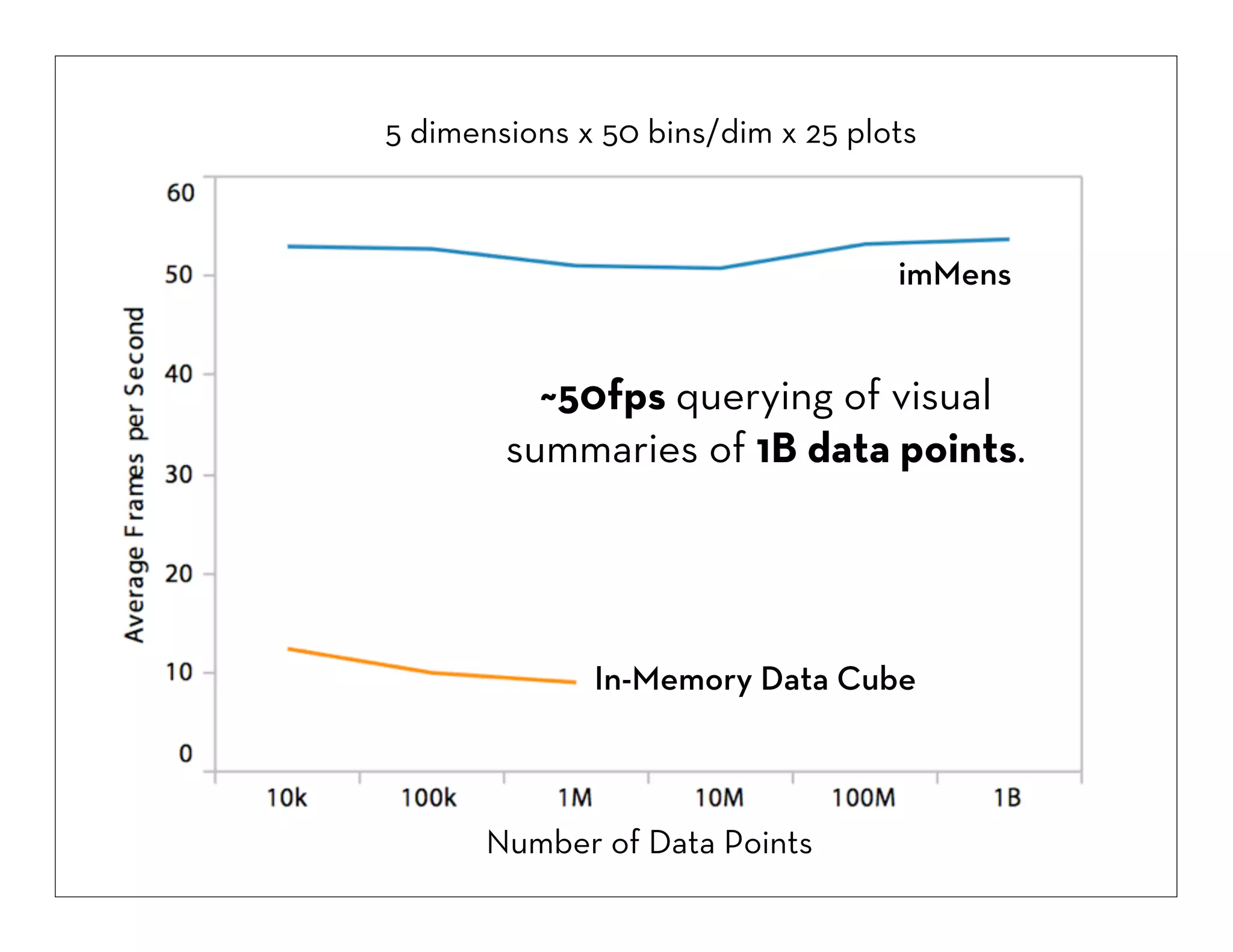
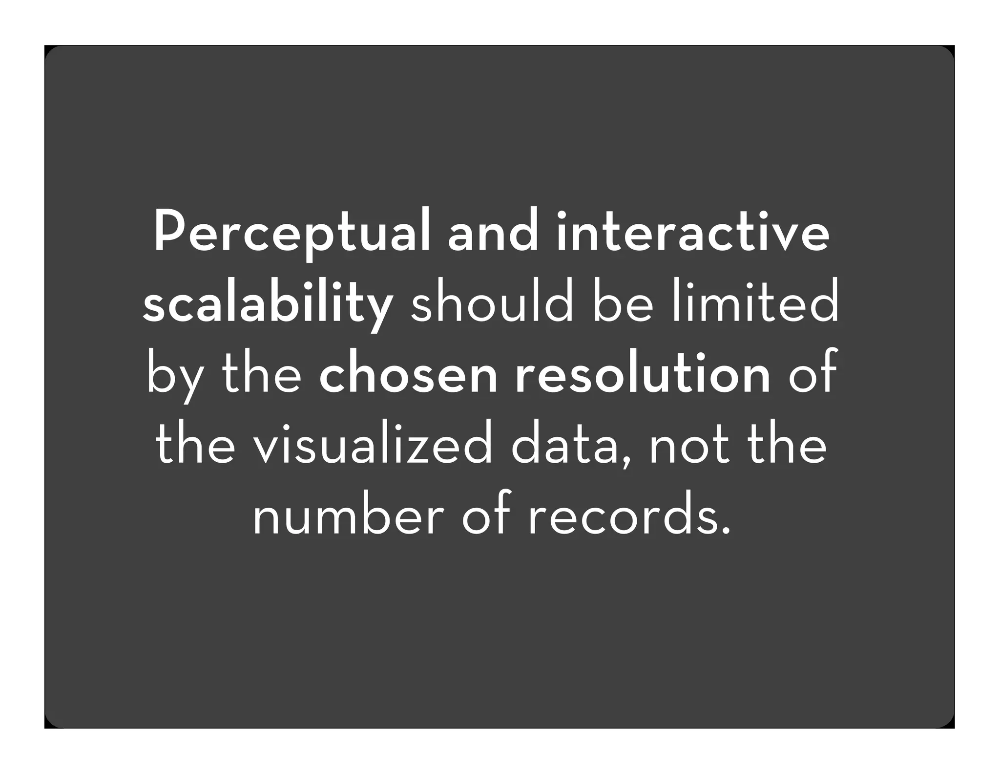
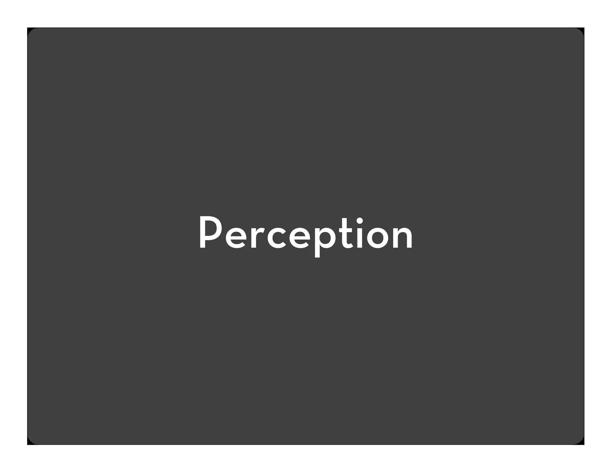
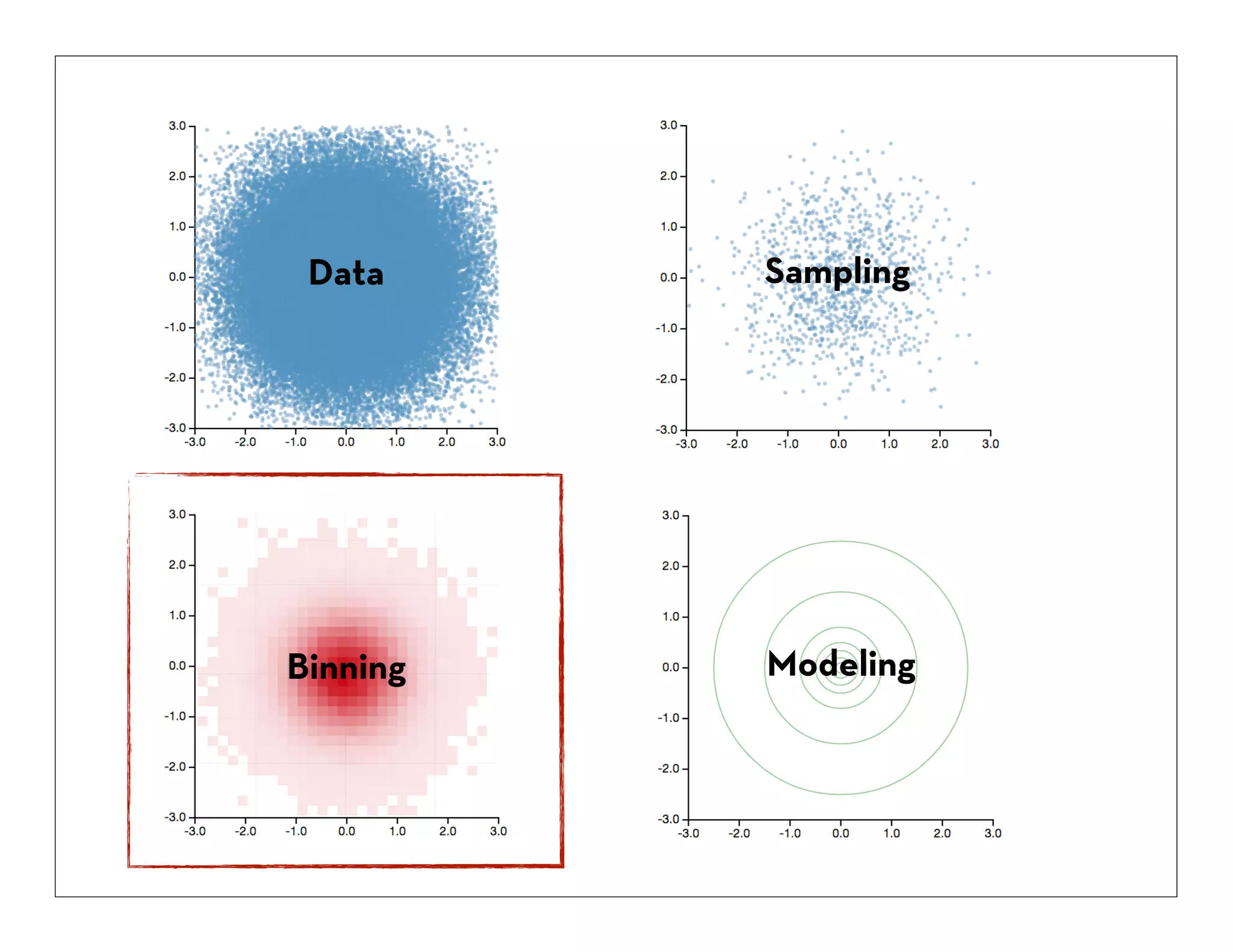
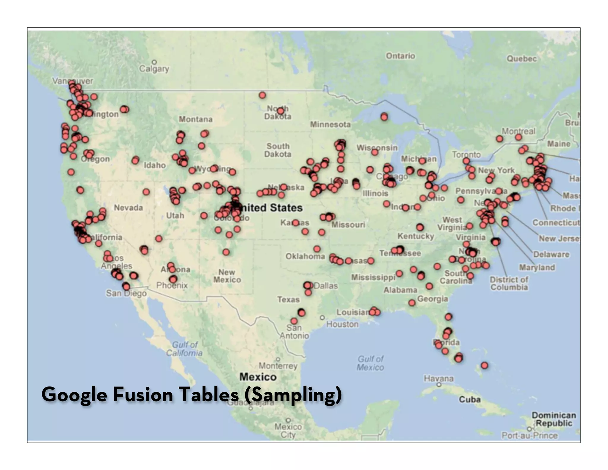
1. The document discusses techniques for visualizing and interacting with billion record databases in real-time. 2. It describes using binning, aggregation, and sampling to summarize large datasets and make them perceptually and interactively scalable. 3. Key techniques discussed include binning data into discrete buckets, aggregating statistics within bins, and using GPU processing and WebGL to enable fast querying and linking of visual summaries across multiple plots of billion record datasets.

1. Visualizing
“Big” Data
Sean Kandel & Jeffrey Heer
Trifacta Inc. @trifacta

2. How can we visualize and
interact with billion+ record
databases in real-time?

3. Two Challenges:
1. Effective visual encoding
2. Real-time interaction

4. Perceptual and interactive
scalability should be limited
by the chosen resolution of
the visualized data, not the
number of records.

5. Perception

6. Data
Sampling
Binning
Modeling

7. Google Fusion Tables (Sampling)

8. imMens (Binned Aggregation)

9. Bin > Aggregate (> Smooth) > Plot
1. Bin Divide data domain into discrete “buckets”
Categories: Already discrete (but check cardinality)
Numbers: Choose bin intervals (uniform, quantile, ...)
Time: Choose time unit: Hour, Day, Month, etc.
Geo: Bin x, y coordinates after cartographic projection

10. Number of Bins?

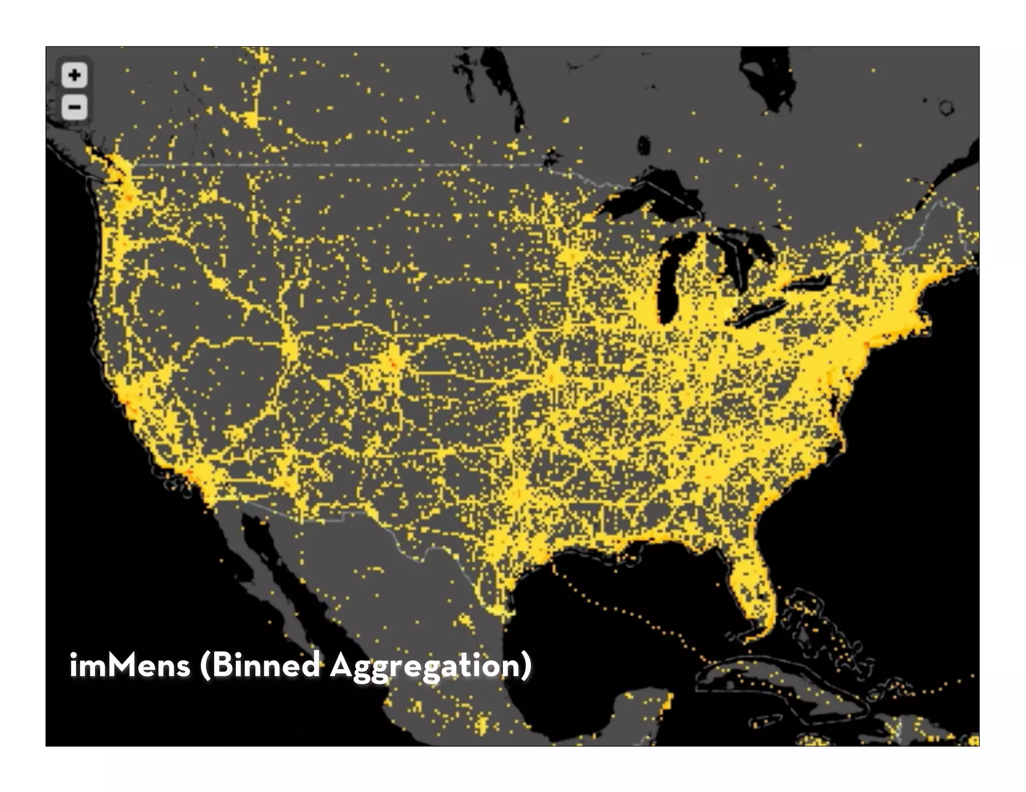
11. Hexagonal or Rectangular Bins?
100,000 Data Points
Hexagonal Bins
Rectangular Bins
Hex bins better estimate density for 2D plots,
but the improvement is marginal [Scott 92], while
rectangles support reuse and query processing.

12. Bin > Aggregate (> Smooth) > Plot
1. Bin Divide data domain into discrete “buckets”
Categories: Already discrete (but check cardinality)
Numbers: Choose bin intervals (uniform, quantile, ...)
Time: Choose time unit: Hour, Day, Month, etc.
Geo: Bin x, y coordinates after cartographic projection
2. Aggregate Count, Sum, Average, Min, Max, ...

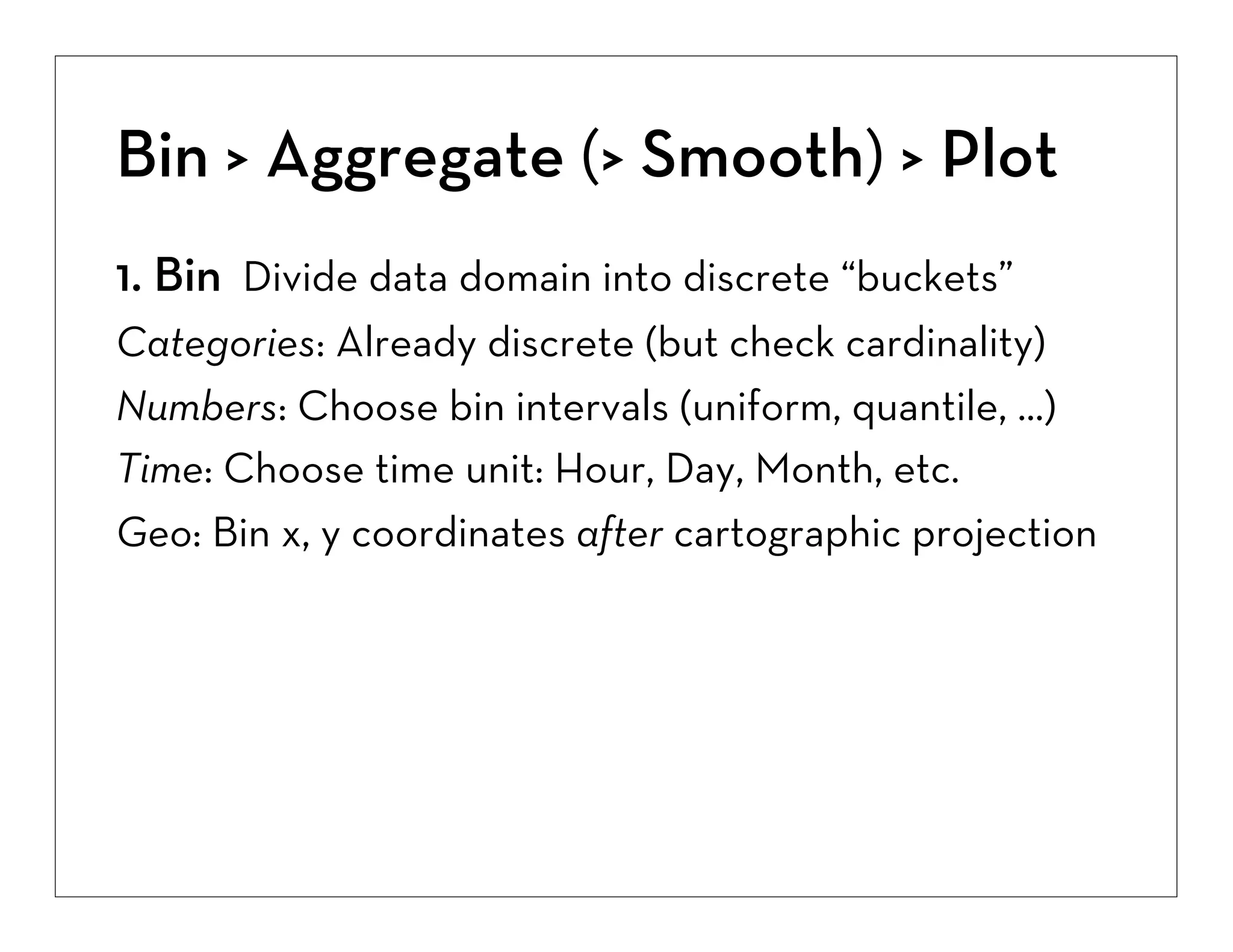
13. Bin > Aggregate (> Smooth) > Plot
1. Bin Divide data domain into discrete “buckets”
Categories: Already discrete (but check cardinality)
Numbers: Choose bin intervals (uniform, quantile, ...)
Time: Choose time unit: Hour, Day, Month, etc.
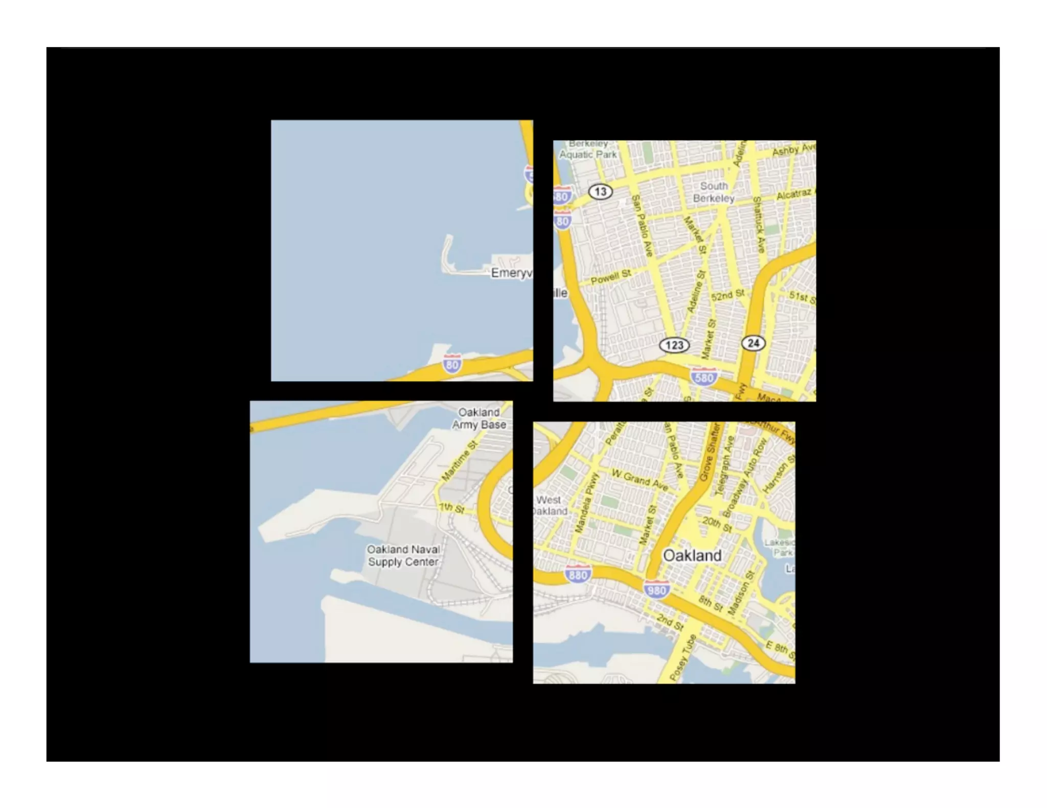
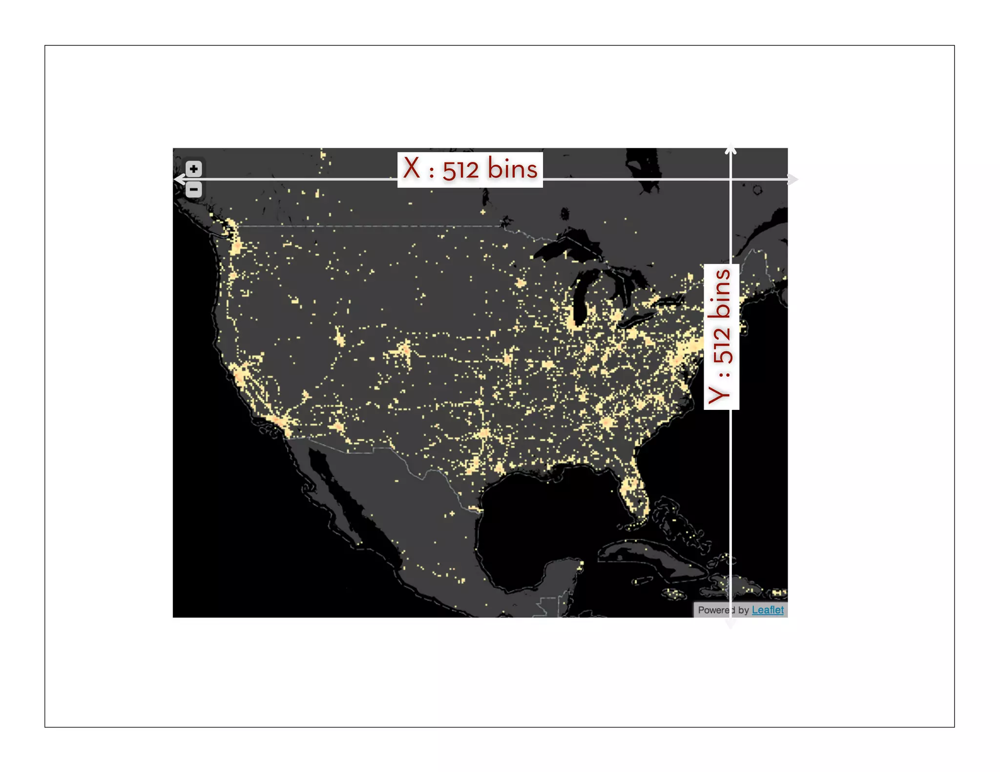
Geo: Bin x, y coordinates after cartographic projection
2. Aggregate Count, Sum, Average, Min, Max, ...
(3. Smooth Optional: smooth aggregates [Wickham ’13])

14. [1] Wickham 2013

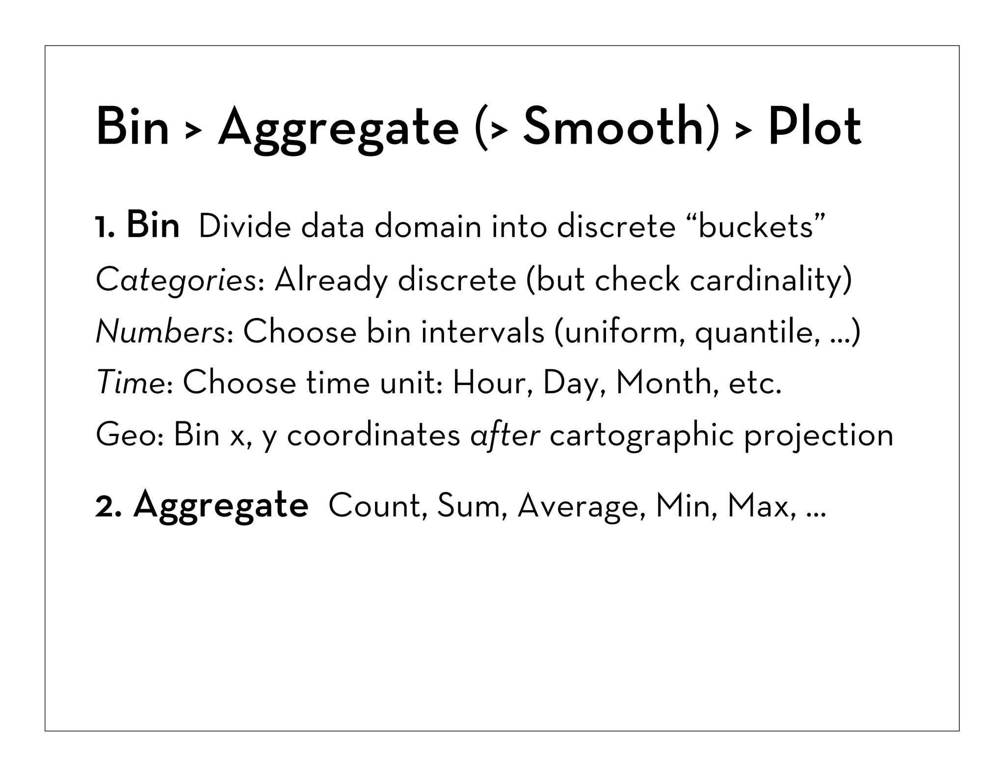
15. Bin > Aggregate (> Smooth) > Plot
1. Bin Divide data domain into discrete “buckets”
Categories: Already discrete (but check cardinality)
Numbers: Choose bin intervals (uniform, quantile, ...)
Time: Choose time unit: Hour, Day, Month, etc.
Geo: Bin x, y coordinates after cartographic projection
2. Aggregate Count, Sum, Average, Min, Max, ...
(3. Smooth Optional: smooth aggregates [Wickham ’13])
4. Plot Visualize the aggregate summary values

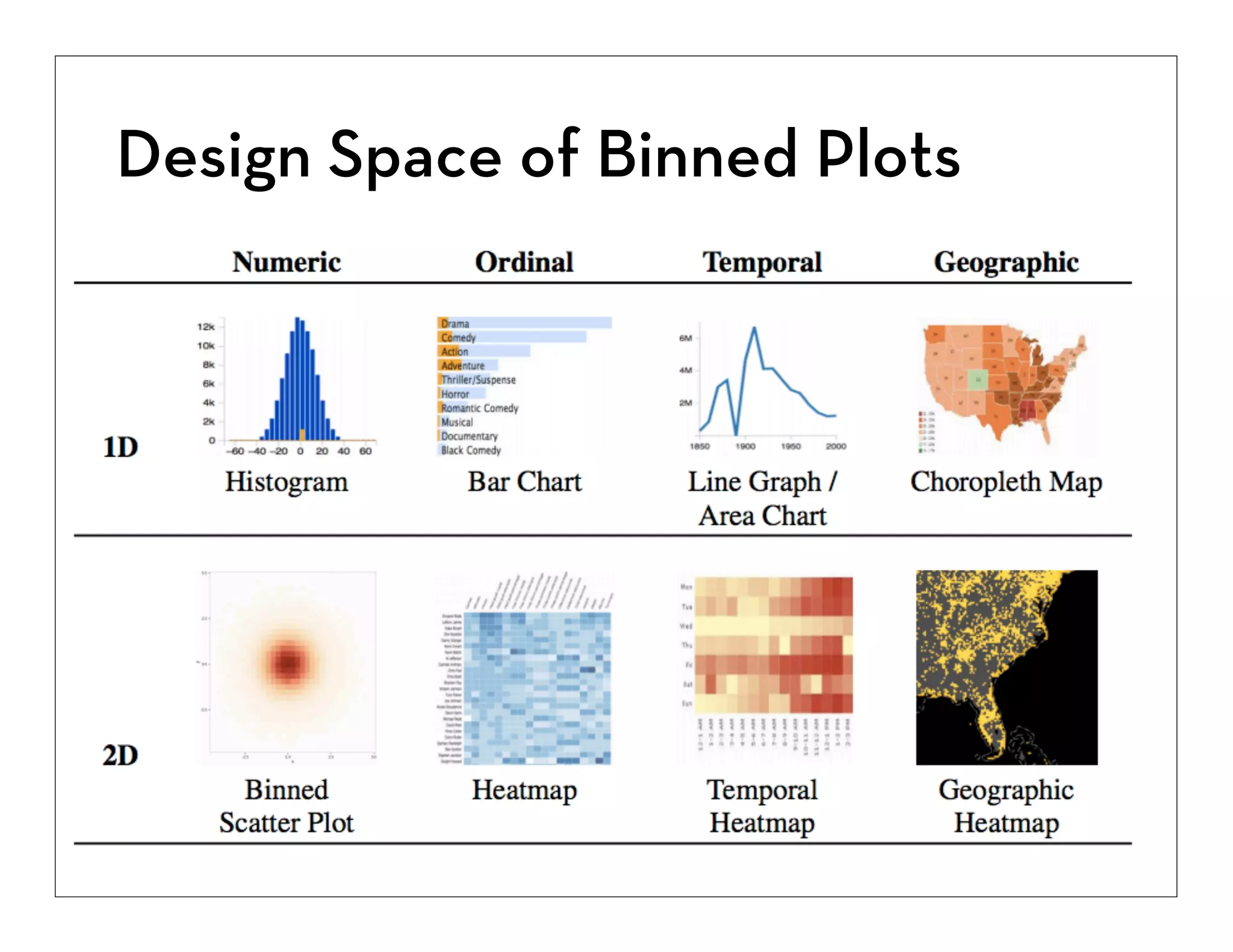
16. Plot: Visual Encoding
Choose Most Effective Encoding [Cleveland & McGill ’84]
1D Plot -> Position or Length Encoding
Histograms, line charts, etc.
2D Plot -> Area or Color Encoding
Spatial dimensions (x, y) already allocated.
While less effective than area for magnitude
estimation, color can be used at the per-pixel level
and provides an overall “gestalt”

17. Standard Color Ramp
Counts near zero are white.
-> Outliers are missed
Add Discontinuity after Zero
Counts near zero remain visible.
-> Outliers can be seen

18. Linear Alpha Interpolation
is not perceptually linear.
Cube-Root Alpha Interpolation
approximates perceptual linearity.

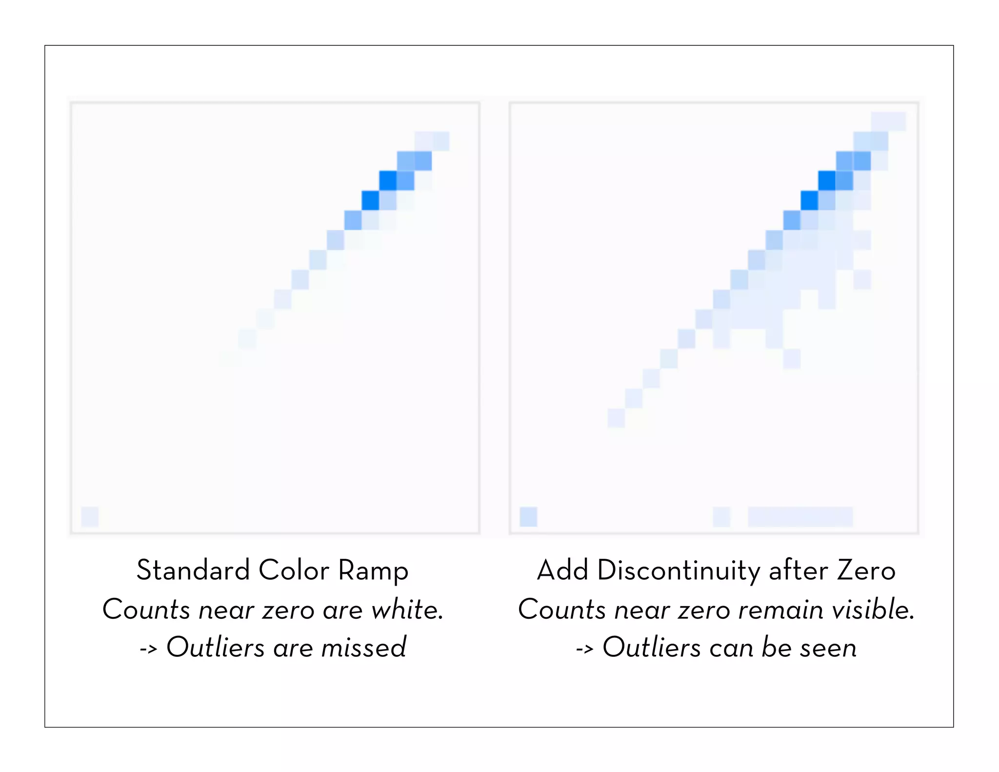
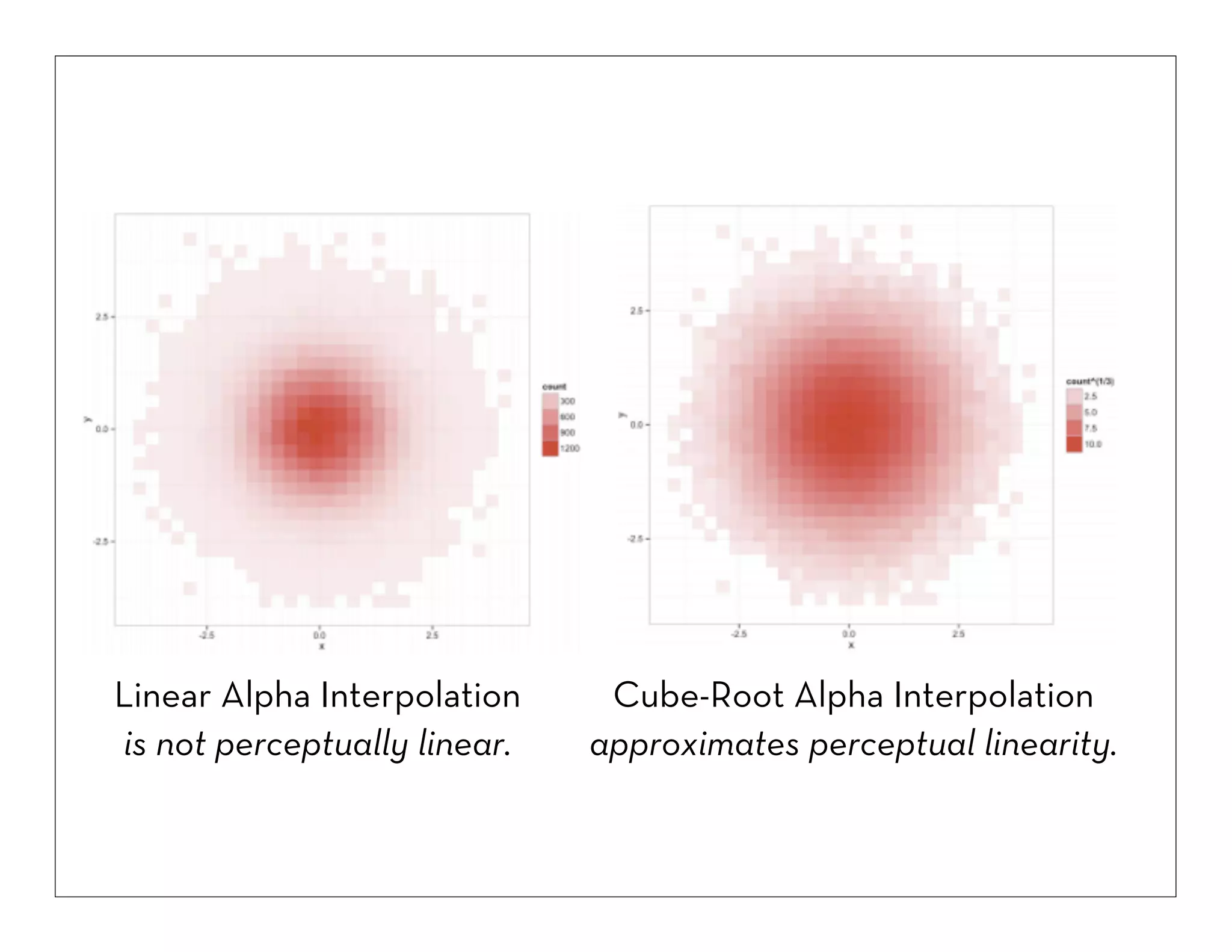
19. Color Encoding
Min. Non-Zero Intensity (α=0.15) [1]
Perceptual Scaling (γ=1/3) [2]
Luminance (in range 0-1) User-Adjustable Min/Max Values [3]
[1] Keep small non-zero values visible (outliers!)
[2] Match color ramp to perceptual distances
[3] Enable exploration across value ranges

20. Design Space of Binned Plots

21. Interaction

22. Interaction Techniques?
1. Select
Detail-on-Demand
2. Navigate Pan & Zoom
3. Query Brush & Link

25. Y
512
…
1023
5-D Data Cube
Month, Day, Hour, X, Y
767
…
X
Month …11
11
…
0
23
…
0
23
…
11
…
0
23
…
1
1
1
0
0
0
Hour
0 1
… 30
0 1
…
30
0 1
256
… 30
Day
12 x 31 x 24 x 512 x 512 = ~2.3 billion cells

26. Y
512
…
1023
Brushing January
Month, Day, Hour, X, Y
767
…
X
Month …11
11
…
0
23
…
0
23
…
11
…
0
23
…
1
1
1
0
0
0
Hour
0 1
… 30
0 1
…
30
0 1
256
… 30
Day
31 x 24 x 512 x 512 = ~195 million cells

29. Multivariate Data Tiles
1. Send data, not pixels
2. Embed multi-dim data

30. Full 5-D Cube
Σ
Σ
Σ
Σ
For any pair of 1D or 2D binned plots, the
maximum number of dimensions needed
to support brushing & linking is four.

31. Y : 512 bins
X : 512 bins

48. ~2.3B bins
Full 5-D Cube
Σ
Σ
Σ
13 3-D Data Tiles
Σ
~17.6M bins
(in 352KB!)

49. Query & Render on GPU via WebGL
Pack data tiles as PNG image files,
bind to WebGL as image textures.

50. Query & Render on GPU via WebGL
Σ
Invoke program for each output bin.
Executes in parallel on GPU.

51. Query & Render on GPU via WebGL
Σ

52. Performance Benchmarks
Simulate interaction:
brushing & linking
across binned plots.
- imMens vs. Profiler
- 4x4 and 5x5 plots
- 10 to 50 bins
Measure time from
selection to render.
Test setup:
2.3 GHz MacBook Pro (4-core)
NVIDIA GeForce GT 650M
Google Chrome v.23.0

53. 5 dimensions x 50 bins/dim x 25 plots
imMens
~50fps querying of visual
summaries of 1B data points.
In-Memory Data Cube
Number of Data Points

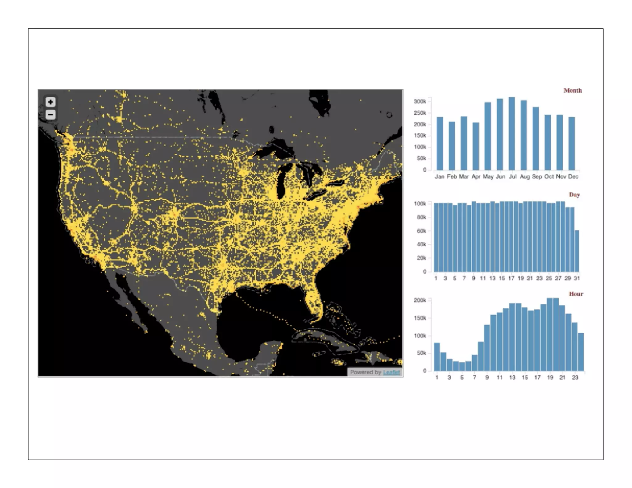
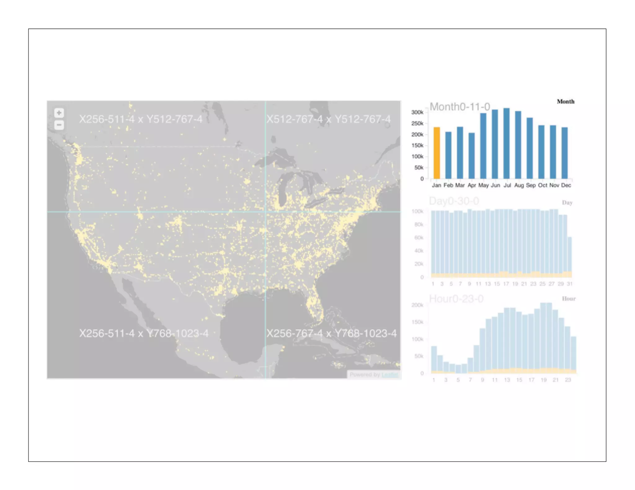
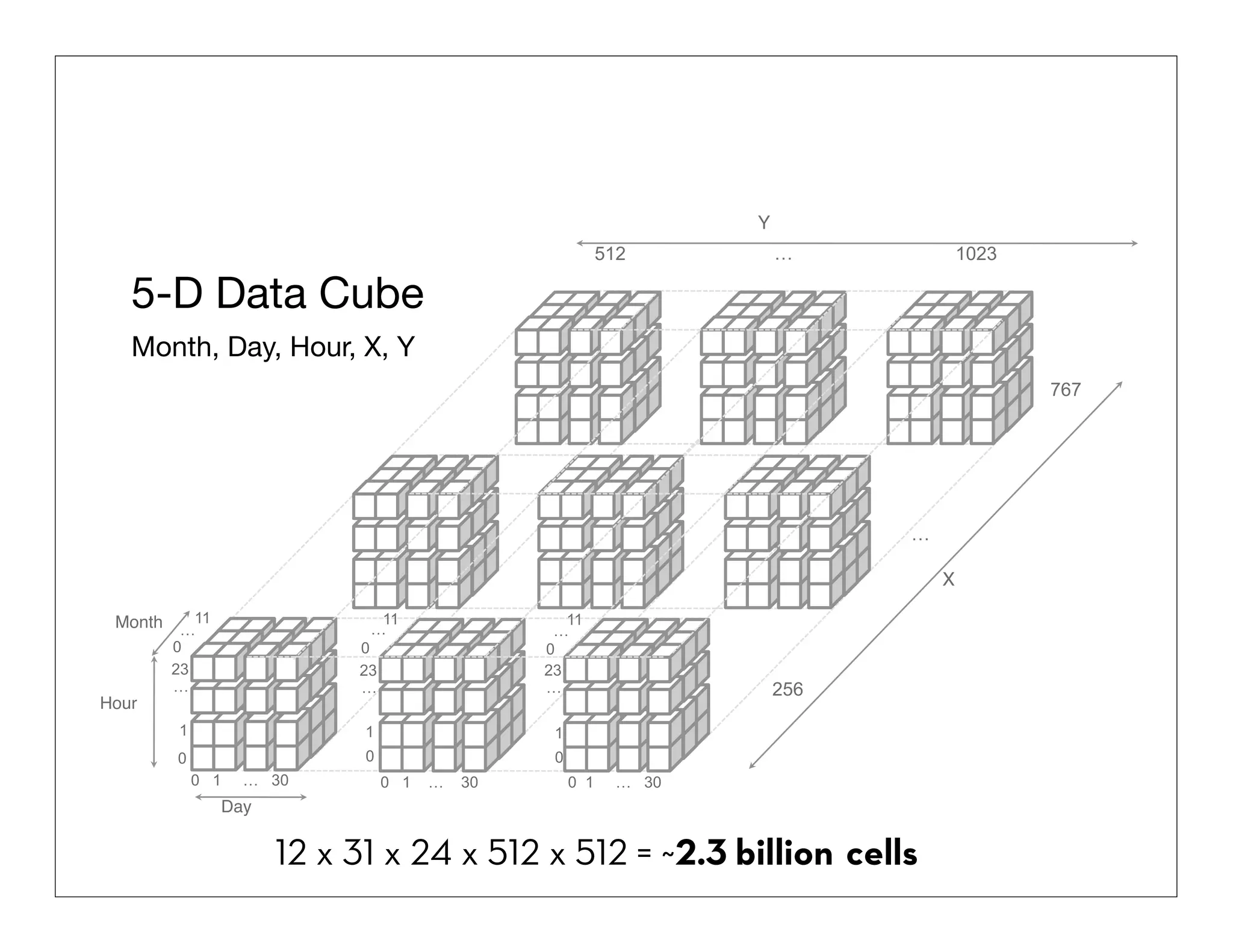
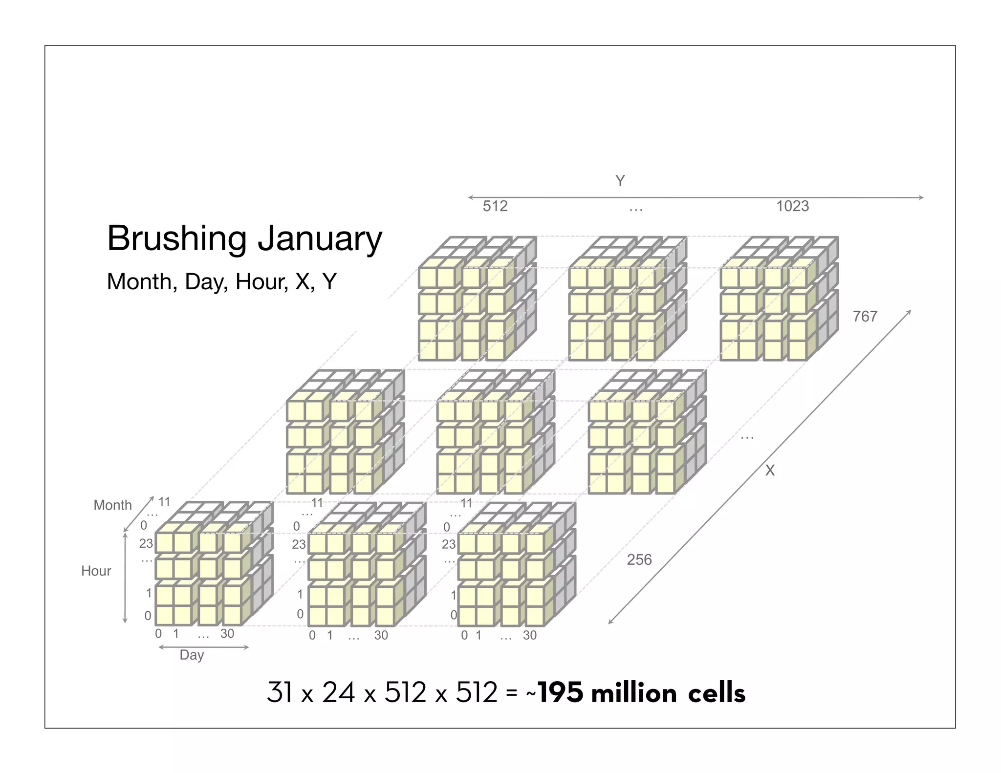
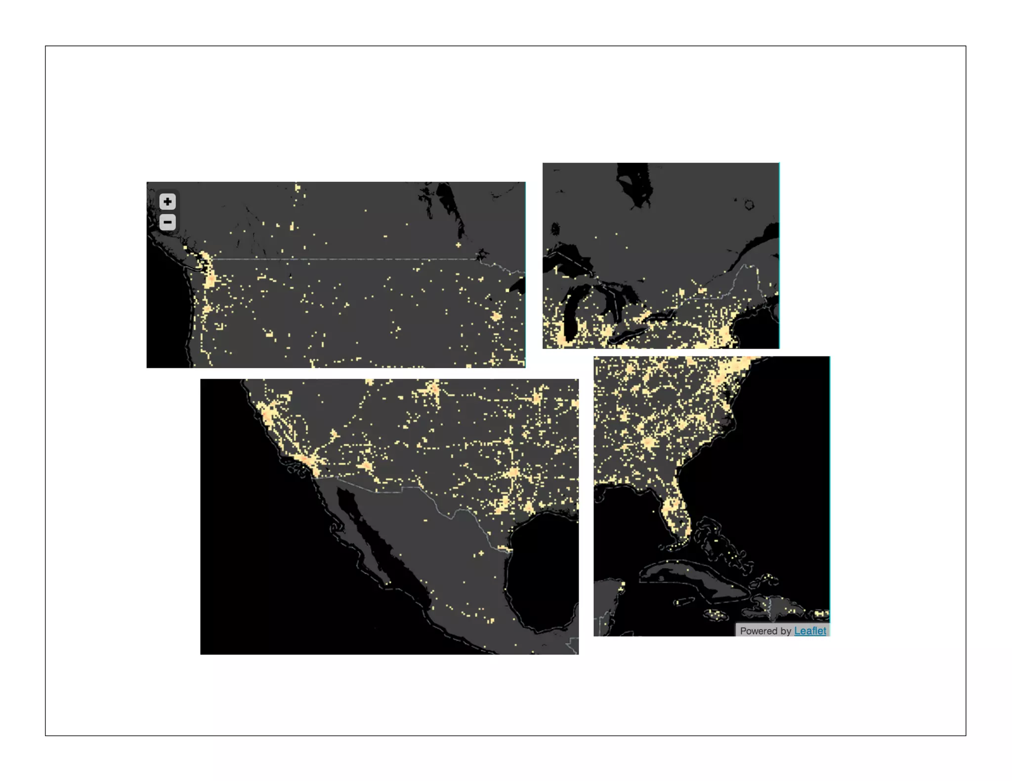
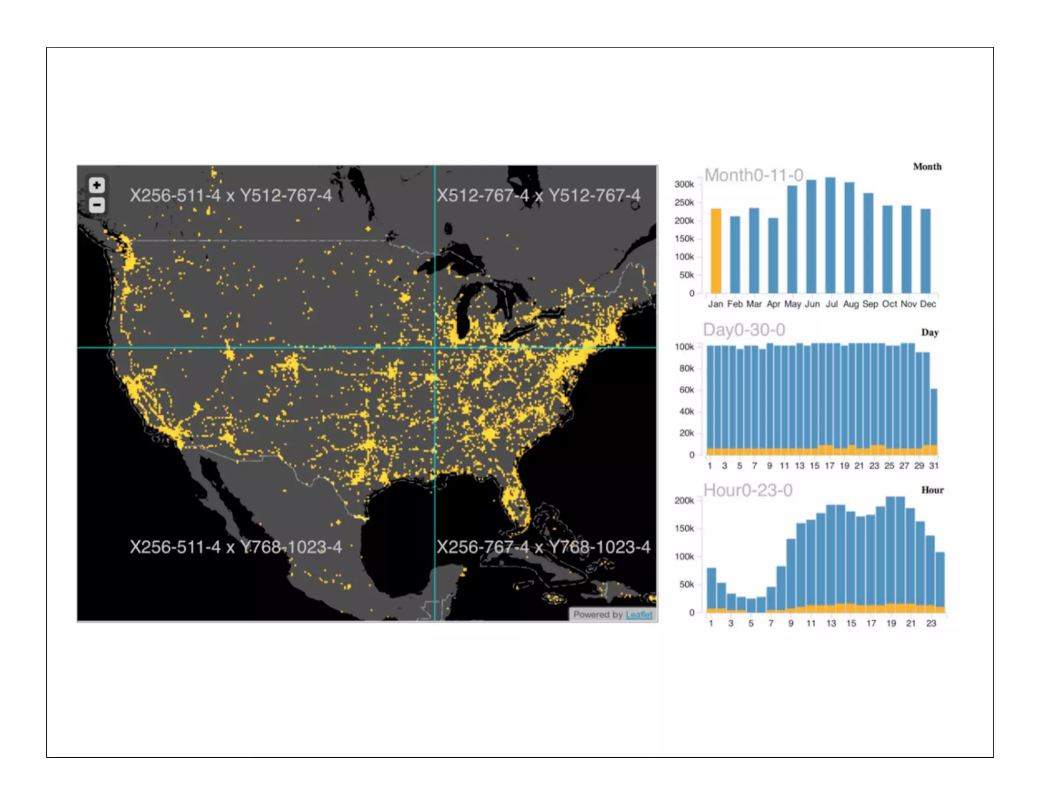
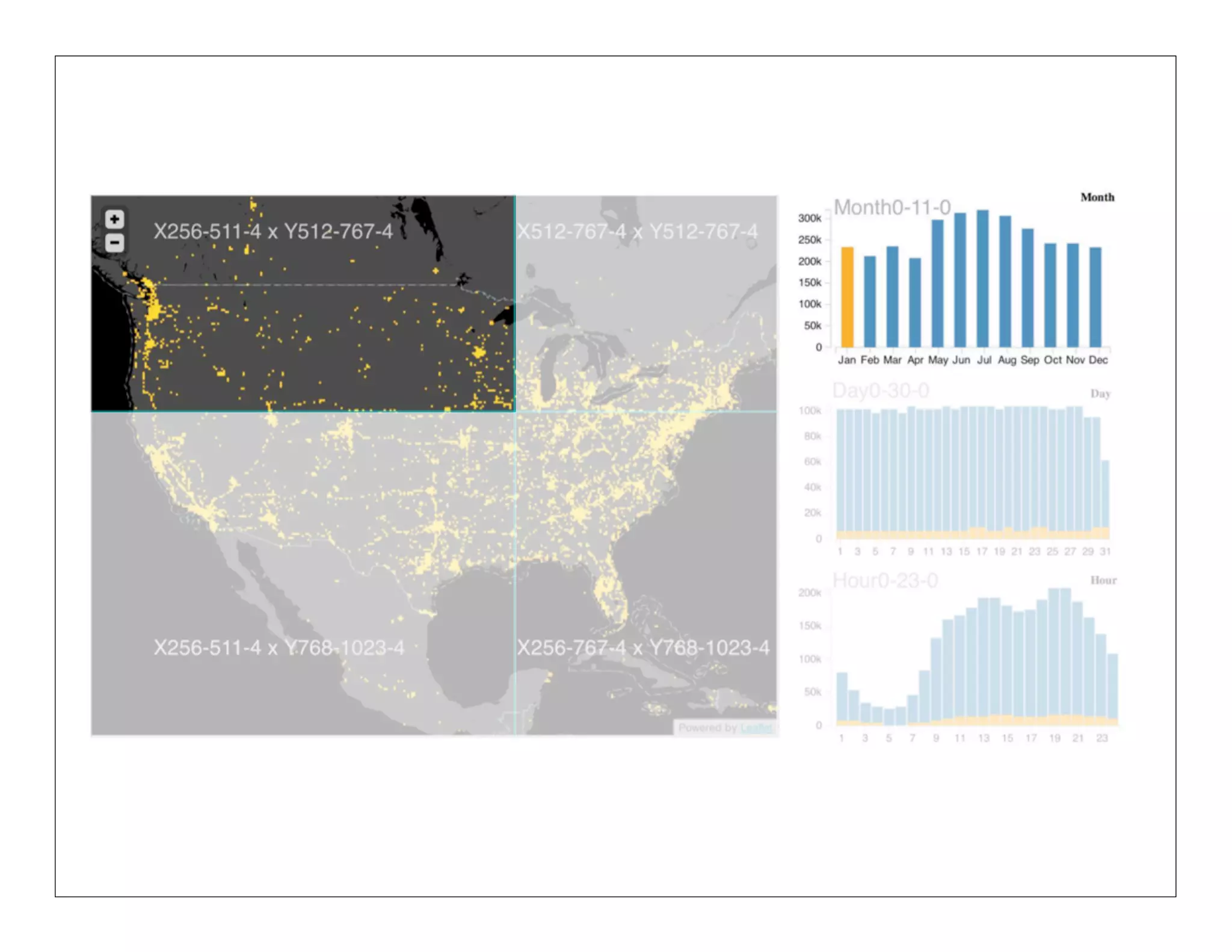
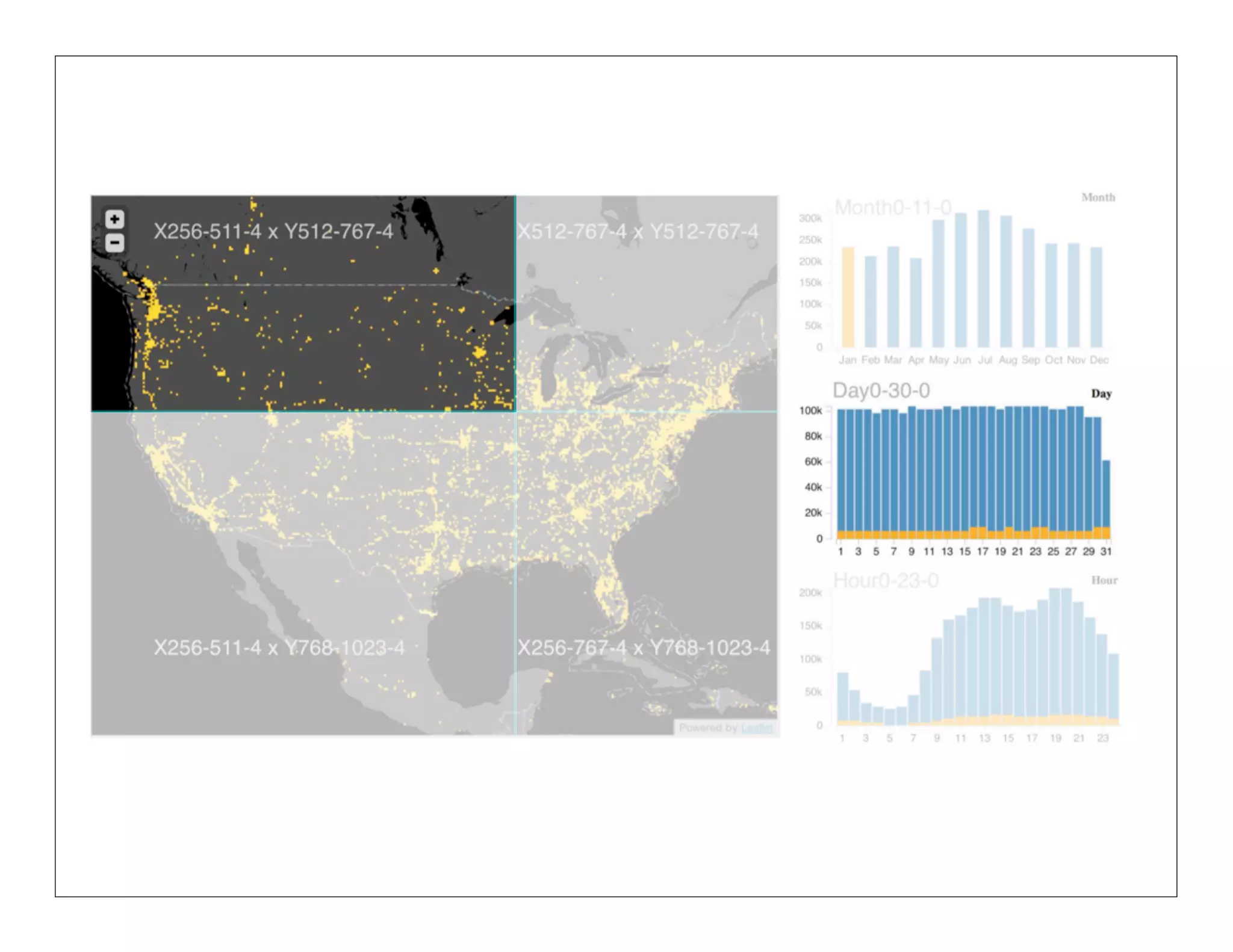
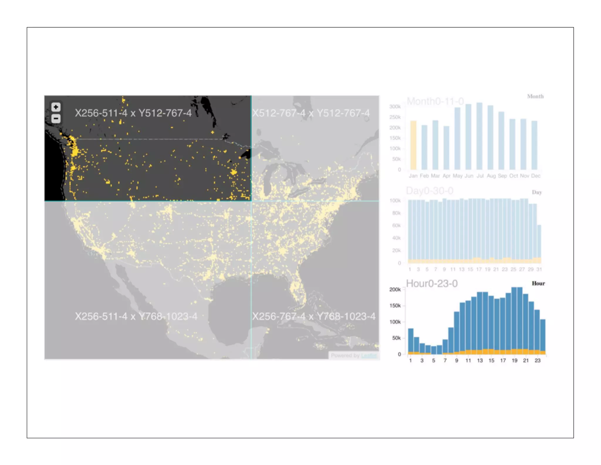
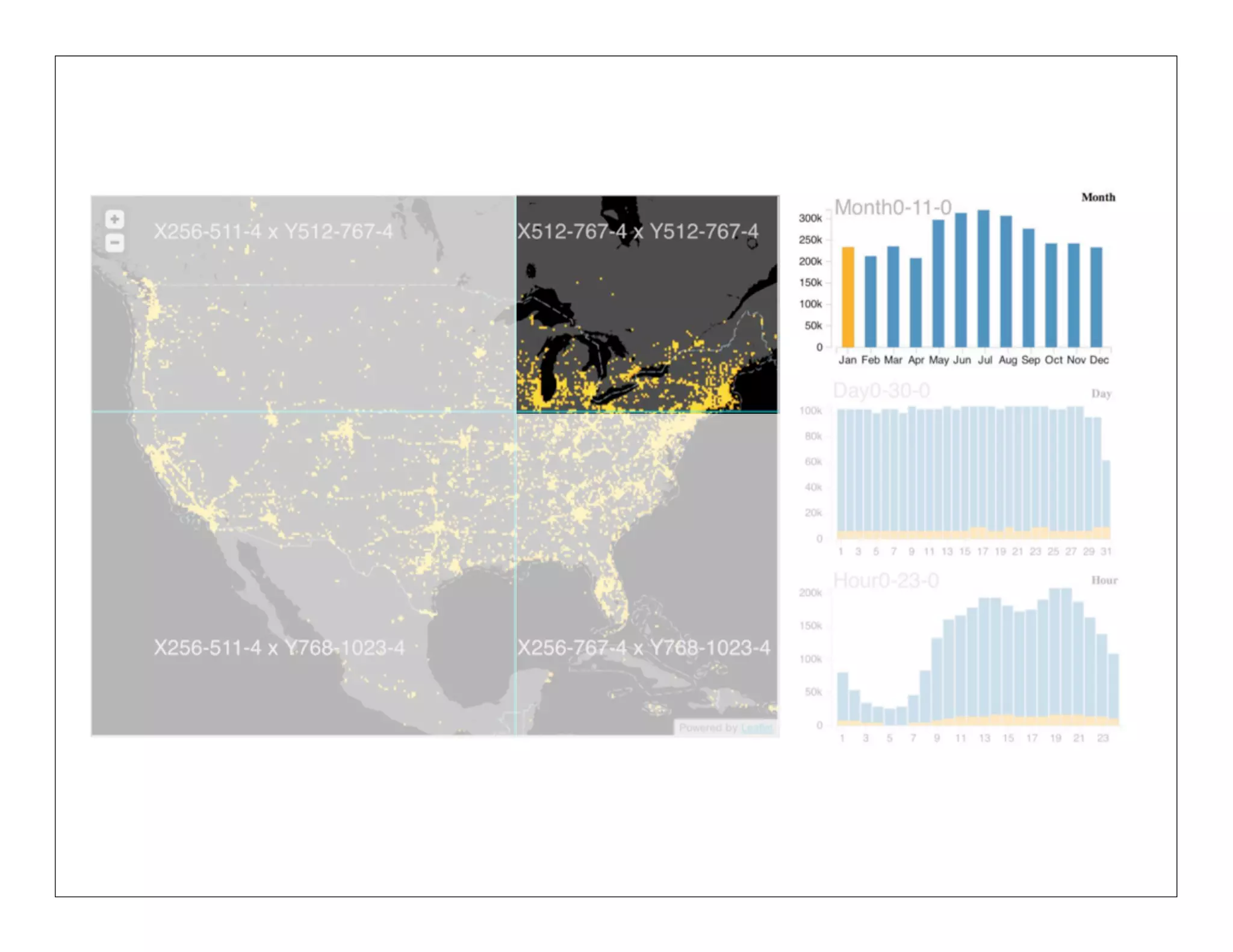
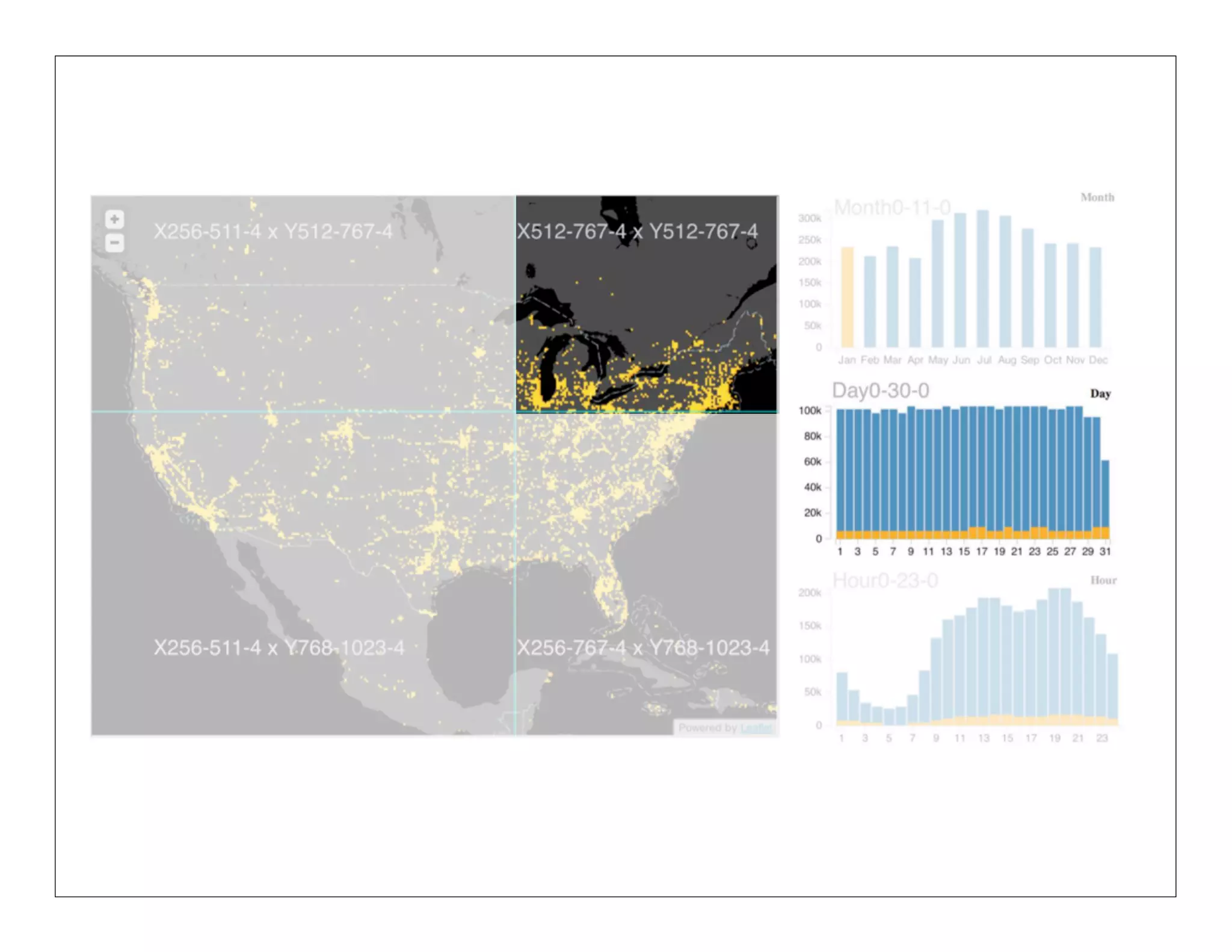
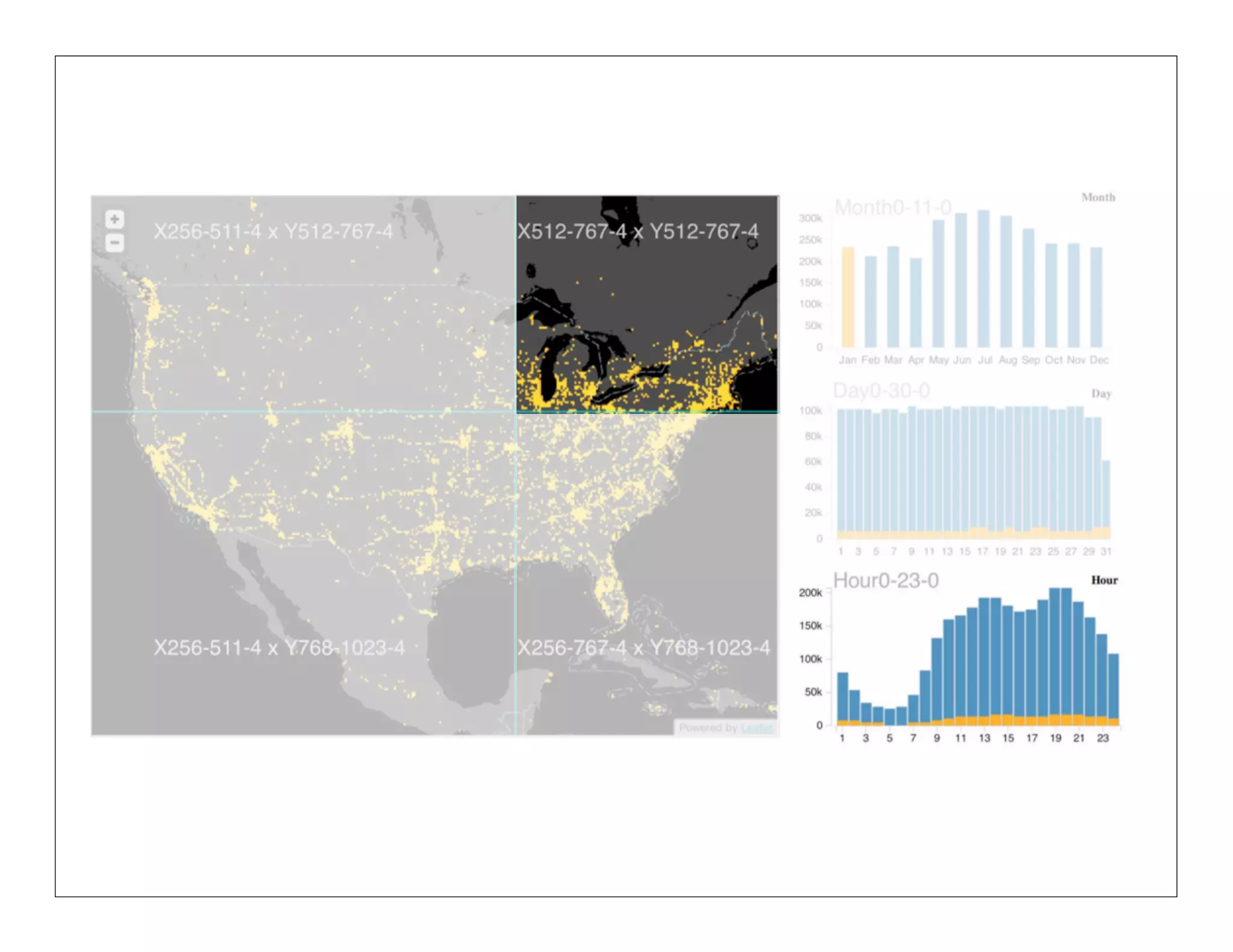
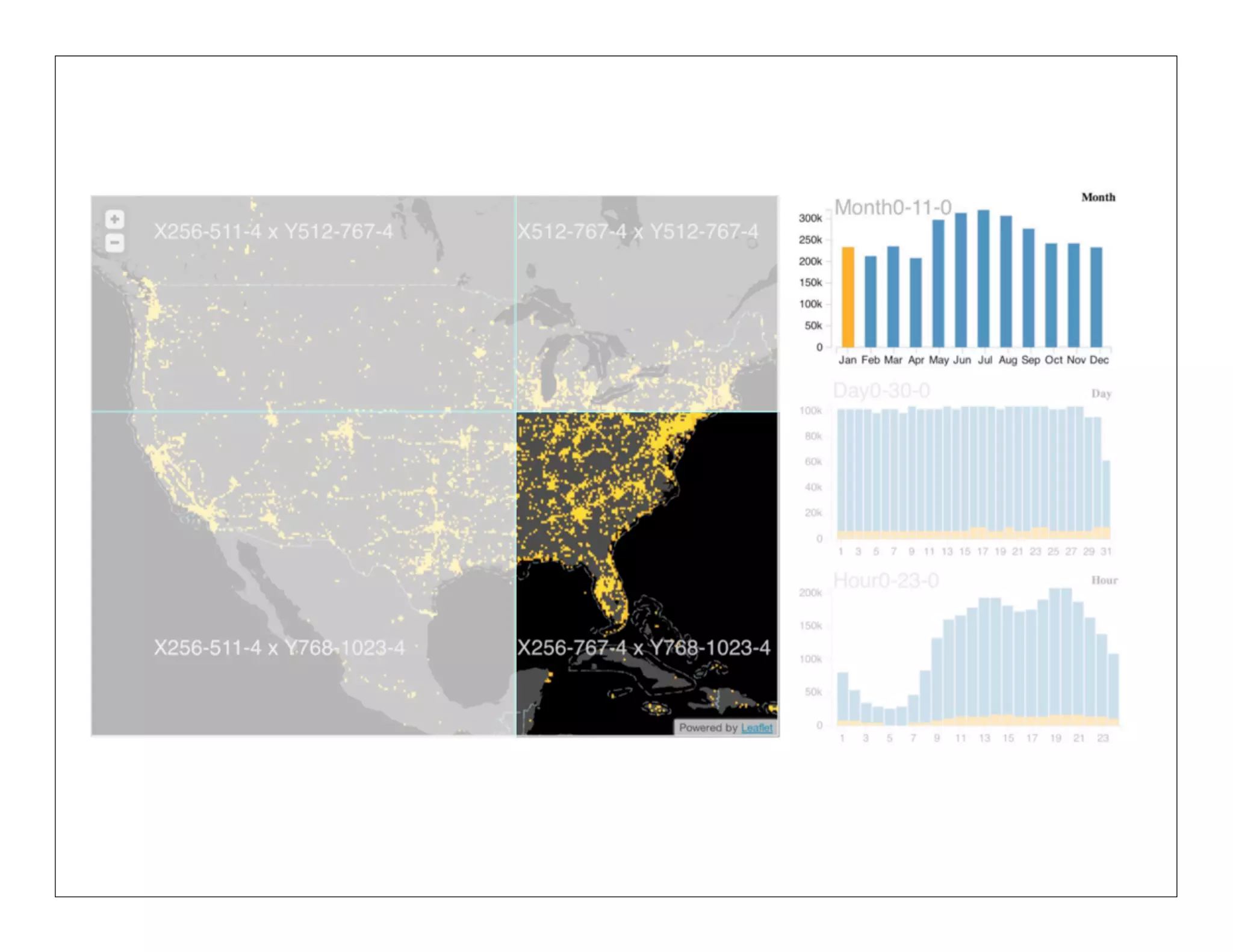
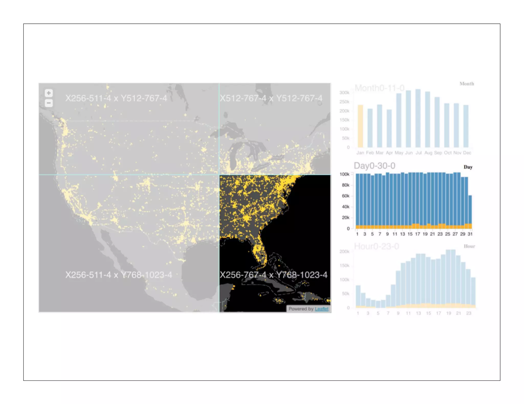
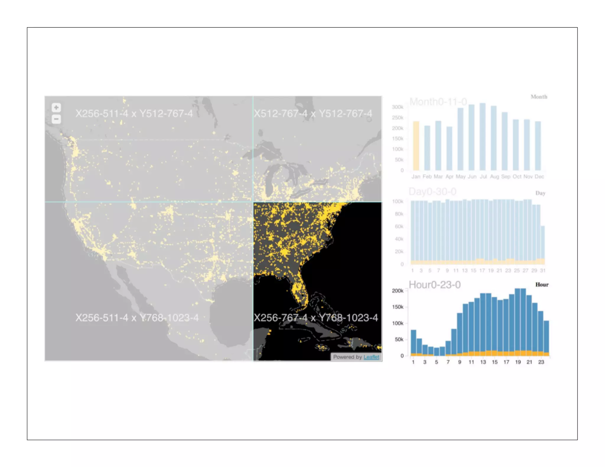
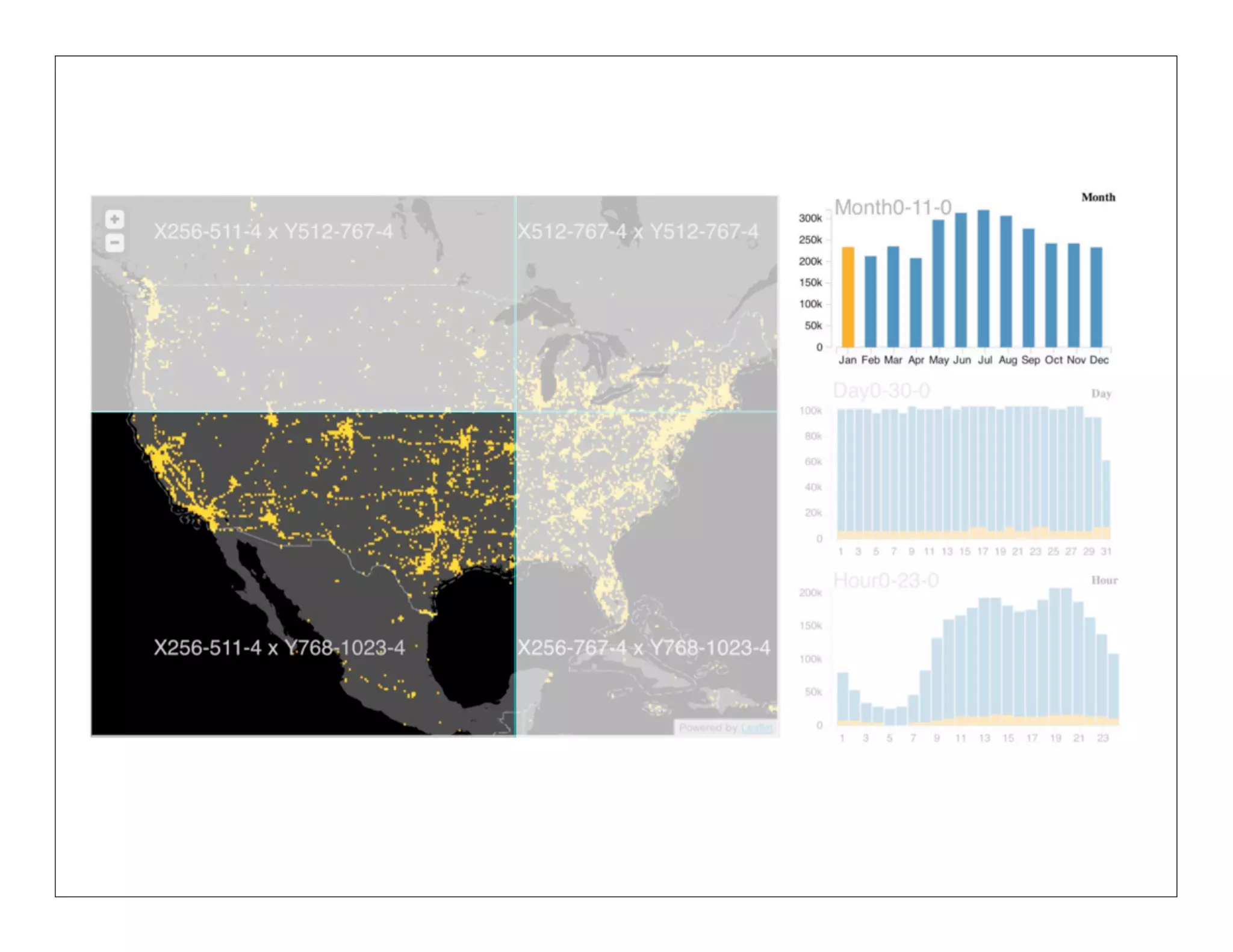
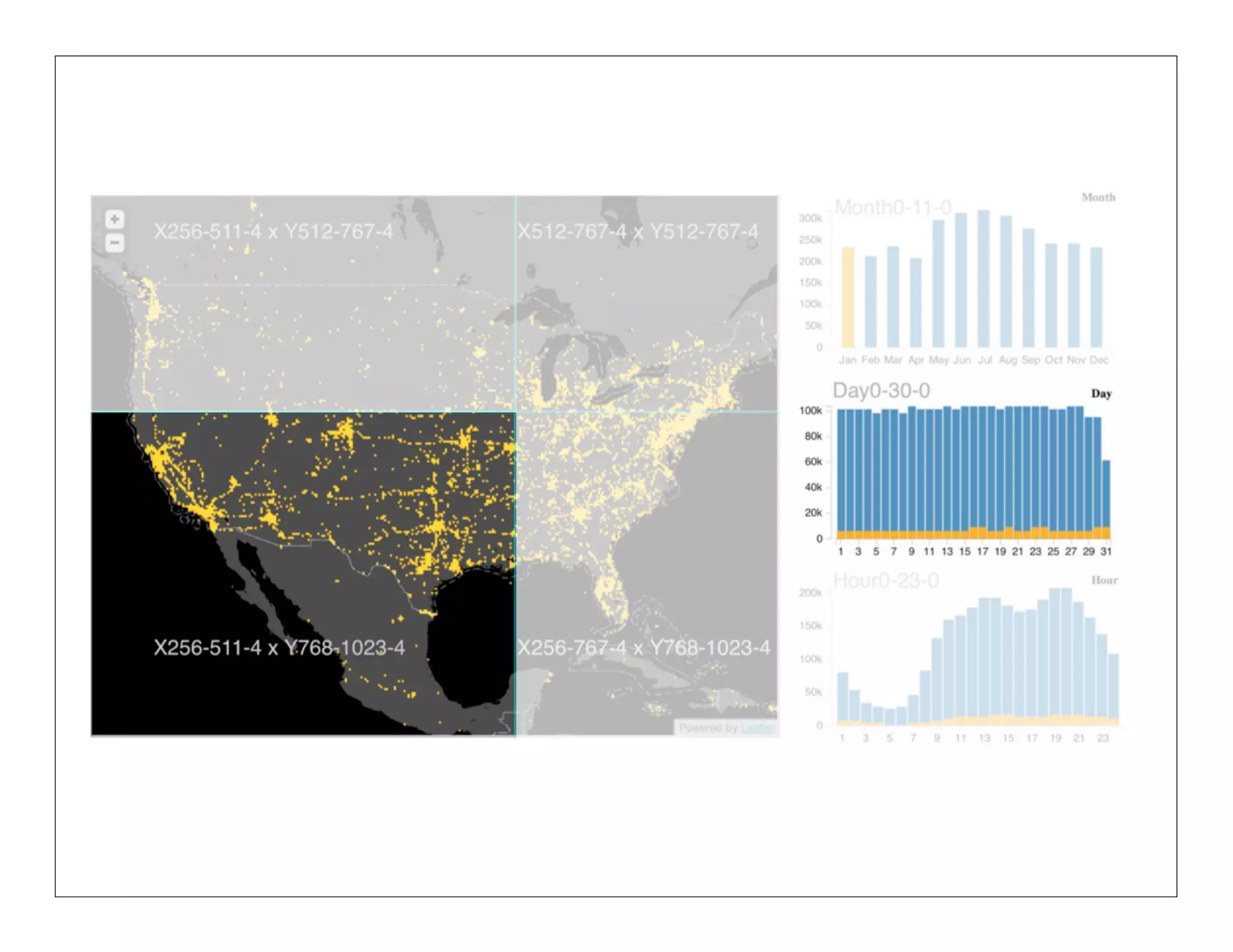
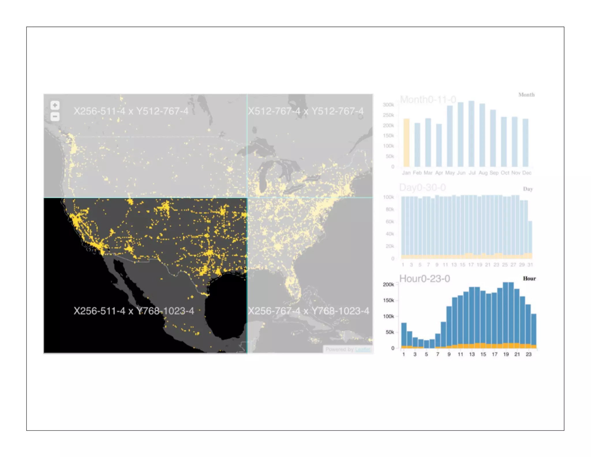
54. NanoCubes
[1] Lins et. al. Infovis 2013
[2] Sismanis et. al. SIGMOD 2002

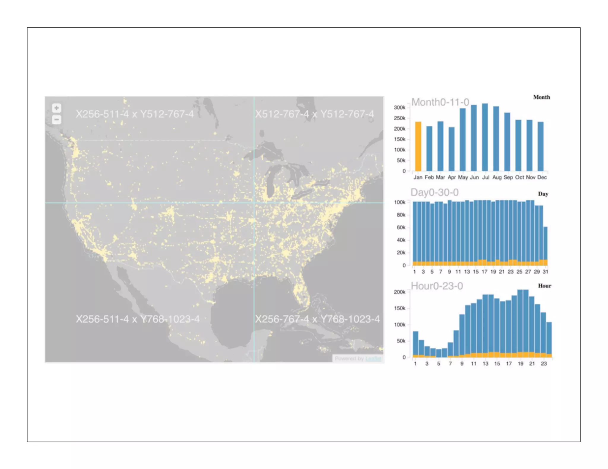
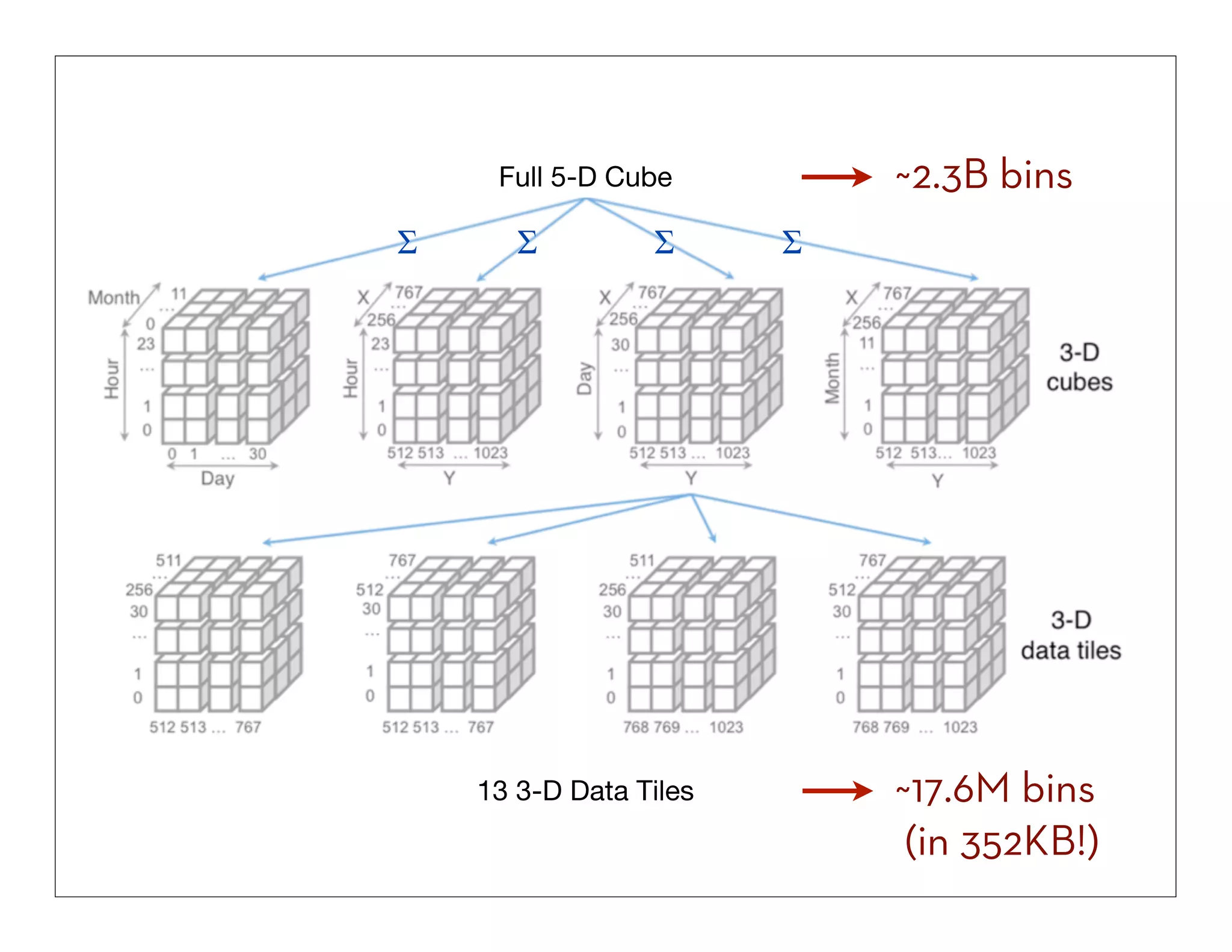
55. NanoCubes
[1] Lins et. al. Infovis 2013

56. Resources
imMens
Tableau Public
BigVis (R)
Nanocubes
BlinkDB
MapD
vis.stanford.edu/projects/immens
tableausoftware.com/public
github.com/hadley/bigvis
nanocubes.net
blinkdb.org
geops.csail.mit.edu/docs/

57. Acknowledgments
Zhicheng “Leo” Liu
Biye Jiang

58. Visualizing
“Big” Data
Sean Kandel & Jeffrey Heer
Trifacta Inc. @trifacta