This document provides parameters used in FLAC analyses for various soil types including silty sand with 20% fines, soft clay, and silt. It summarizes the methodology used to determine saturated unit weight, dry unit weight, porosity, specific gravity, elastic modulus, shear modulus, bulk modulus, permeability, and other parameters for each soil type based on reference tables and equations. Parameters like friction angle, cohesion, dilation angle, and constants for the Finn model are also selected from the references for each soil. Aggregate pier parameters are determined by selecting stiffness 8 times greater than the surrounding soils.

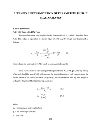
1. 262
APPENDIX A DETERMINATION OF PARAMETERS USED IN
FLAC ANALYSES
A.1 Soil Parameters
A.1.1 Silty Sand with 20% Fines
The typical saturated unit weight value for this type of soil is 120 lb/ft3
(based on Table
A.1). This value is equivalent to density (ρsat) of 3.73 slug/ft3
, which was determined as
follows:
3
2
3
73.3
sec
185.32
120
ft
slug
ft
ft
lb
g
sat
sat ==
γ
=ρ (A.1)
(Note: slug is the unit used in FLAC, which is equivalent to lb-sec2
/ft)
Since FLAC analyses were configured for groundwater (CONFIGgw), the dry density
of the soil should be used. FLAC will compute the saturated density of each element, using the
known values of the density of water, the porosity, and the saturation. The dry unit weight of
soil can be determined by the following equations:
( )
e
e
G
w
sat
s −
+
=
γ
γ 1
(A.2)
( )e
G ws
d
+
=
1
γ
γ (A.3)
where:
γsat = the saturated unit weight of soil
γw = the unit weight of water
e = void ratio

2. 263
Gs = the specific gravity of soil
γd = the dry unit weight of soil
Based on Table A.2, a value of void ratio (e) of 0.7 was selected. Based on the known
values of γsat (=120 pcf), e (=0.7), and γw (=62.4 pcf), Gs = 2.57 was obtained by using equation
(A.1). This value was used in equation (A.2) and γd = 94 pcf was obtained, which is equivalent
to 2.93 slug/ft3
.
Based on the selected void ratio (e) of 0.7, the porosity of soil can be determined using
equation (A.4) and n of 0.412 was obtained.
e
e
n
+
=
1
(A.4)
Table A.3 shows the relationship between Standard Penetration Test N-values, (N1)60
versus friction angle (φ). Based on this relationship, the values of 10 blows/ft and 30° were
used for (N1)60 and φ, respectively.
Tables A.4 and A.5 show the typical values of elastic modulus (E) and Poisson’s ratio
(ν) for various types of soil. Based on these tables, the values of 15 MPa (315,000 psf) and 0.3
were selected for E and ν, respectively.
The values of E and ν were then used to calculate the bulk modulus (K) and the shear
modulus (G) using the following equations:
( )ν−
=
213
E
K (A.5)
( )ν+
=
12
E
G (A.6)
By using equations (A.5) and (A.6) the following parameters were obtained:
K = 315,000 psf
G = 118,125 psf

3. 264
Table A.6 shows the typical values of dilation angle (ψ). The dilation angle of 0° was
selected in the FLAC analysis.
Based on Table A.7, permeability (k) of 10-4
cm/sec. (3.28*10-6
ft/sec.) was selected.
Equation (A.9) was used to determine the value of FLAC permeability, which result in the
value of 5.26*10-8
ft3
-sec/slug.
w
k
typermeabiliFLAC
γ
= (A.7)
A.1.2 Soft Clay
The typical saturated unit weight (γsat) value for this type of soil is 110 pcf (based on
Table A.1), which is equivalent to density (ρsat) of 3.42 slug/ft3
. Based on Table A.2, a value of
void ratio (e) of 1.1 was selected. By using equation (A.4), porosity (n) of 0.524 was obtained.
Based on the known values of saturated unit weight (γsat) of 110 pcf, void ratio (e) of 1.1, and
unit weight of water (γw) of 62.4 pcf, specific gravity (Gs) of 2.60 was obtained by using
equation (A.2). This value was used in equation (A.3) and dry unit weight (γd) of 77 pcf was
obtained, which is equivalent of 2.40 slug/ft3
.
Table A.8 shows the relationship between SPT (Standard Penetration Test) N-values
versus consistency of clay soil. Based on this relationship, (N1)60 of 4 blows/ft was selected for
soft clay.
Table A.9 shows the typical values of strength properties. Therefore, the values of 10
kPa (210 psf) and 17° were selected for cohesion (c) and friction angle (φ), respectively.
Based on Tables A.4 to A.6, the following values were selected for soft clay:
E = 5 MPa = 105,000 psf, ν = 0.414, and ψ = 0°
The above values were then used to calculate the bulk modulus (K) and the shear
modulus (G) using equations (A.5) and (A.6). The following results were obtained:
K = 204,421 psf
G = 37,118 psf

4. 265
Based on Table A.7, permeability (k) of 10-7
cm/sec. (3.28*10-9
ft/sec.) was selected.
Equation (A.7) results in the value of FLAC permeability of 5.26*10-11
ft3
-sec/slug.
A.1.3 Silt
Based on the Tables A.1 to A.6 and A.8 to A.9, the following values were selected and
used in FLAC analysis:
γsat = 115 pcf ⇔ ρsat = 3.57 slug/ft3
e = 0.9 ⇔ n = 0.474
γd = 85 pcf ⇔ ρd = 2.65 slug/ft3
(N1)60 = 8 blows/ft
c = 3 kPa = 63 psf
φ= 25° ⇔ ν = 0.4
E = 10 MPa = 210,000 psf
ψ = 0°
The bulk modulus (K) and the shear modulus (G) were calculated using equations (A.5)
and (A.6). The following results were obtained:
K = 261,268 psf
G = 76,865 psf
Based on Table A.7, permeability (k) of 10-6
cm/sec. (3.28*10-8
ft/sec.) was selected.
Equation (A.7) results in the value of FLAC permeability of 5.26*10-10
ft3
-sec/slug.
A.1.4 Determination of Parameters Used in Finn Model
As noted in Chapter 5, equations suggested by Byrne (1991) were used in the FLAC
analyses. Based on the selected (N1)60 values the constant C1 and C2 can be computed.

5. 266
( ) 25.1
6011 7.8
−
= NC (A.8)
1
2
4.0
C
C = (A.9)
Therefore, for silty sand the following values were used:
C1 = 0.49
C2 = 0.82
For soft clay, the following values were used:
C1 = 1.54
C2 = 0.26
For silt, the following values were used:
C1 = 0.65
C2 = 0.62
A.2 Aggregate Pier Parameters
As noted previously in Chapter 5, an angle of friction (φ) of 50° was selected for the
aggregate piers. Also selected the use of aggregate pier stiffness of 8 times stiffer than that of
the surrounding soils. Therefore, the value of elastic modulus of 2,520,000 psf and 1,680,000
psf for the aggregate pier were used. These values are eight times stiffer than the elastic
modulus of soil (315,000 psf and 210,000 psf for silty sand and silt, respectively).
Based on equation (5.6), the elastic modulus can be calculated. For silty sand, the elastic
modulus of aggregate pier is:
( ) psfE 625,933
2.25
13.18*000,31507.7*000,520,2
=
+
=
By using equations (A.5) and (A.6) and Poisson’s ratio (ν) of 0.2, the following values
were obtained:

6. 267
K = 501,299 psf
G = 392,412 psf
For silt,
( ) psfE 417,622
2.25
13.18*000,21007.7*000,680,1
=
+
=
and
K = 334,199 psf
G = 261,608 psf
Based on Table A.6, dilation angle of 0° was used.
The saturated unit weight of the aggregate pier is 147 pcf (ρsat = 4.57 slug/ft3
) and the
dry unit weight is 136 pcf (ρd = 4.23 slug/ft3
). These values correspond to e = 0.25 (n = 0.2)
and Gs = 2.69.
Based on Table A.7, permeability (k) of 10-1
cm/sec. (3.28*10-3
ft/sec.) was selected,
which corresponds to FLAC permeability of 5.26*10-5
ft3
-sec/slug.
A.3 Water Parameters
As noted previously, for uncoupled flow-mechanical approach, the flow calculation can
be set in flow-only mode (SET flow on, SET mech off), and then in mechanical-only mode
(SET flow off, SET mech on), to bring the model into equilibrium. For the latter, Kw is set to
zero, while for the former, Kw should be adjusted to a
wK by using the equation (4.29).
Therefore, for silty sand,
( )
psfK a
w 662,193
3/125,118*4000,315
1
10*2.4
412.0
412.0
7
=
+
+
=

7. 268
For soft clay,
( )
psfK a
w 582,132
3/118,37*4421,204
1
10*2.4
524.0
524.0
7
=
+
+
=
For silt,
( )
psfK a
w 601,171
3/865,76*4268,261
1
10*2.4
474.0
474.0
7
=
+
+
=
Once, the system is brought into equilibrium, bulk modulus of water (Kw) of 108
Pa (=
2.1 * 106
psf) was used. The unit weight of water used in FLAC analysis is equal to γw = 62.4
pcf (ρw = 1.94 slug/ft3
).
For a coupled flow-mechanical problem (SET flow on, SET mech on), the value of Kw
should be adjusted that the value of Rk is ≤ 20 by using equation (4.27). Since this case was
analyzed only for silty sand soil, the value of Rk becomes
( )
psfK
K
w
w
730,995,3
3/125,118*4000,315
412.0
20 =⇔
+
=

8. 269
Table A.1 Typical values of unit weights (after Coduto, 2001)
Soil type
Above groundwater
table (lb/ft3
)
Below groundwater
table (lb/ft3
)
GP – Poorly-graded gravel 110 – 130 125 – 140
GW – Well-graded gravel 110 – 140 125 – 150
GM – Silty gravel 100 – 130 125 – 140
GC – Clayey gravel 100 – 130 125 – 140
SP – Poorly-graded sand 95 – 125 120 – 135
SW – Well-graded sand 95 – 135 120 – 145
SM – Silty sand 80 – 135 110 – 140
SC – Clayey sand 85 – 130 110 – 135
ML – Low plasticity silt 75 – 110 80 – 130
MH – High plasticity silt 75 – 110 75 – 130
CL – Low plasticity clay 80 – 110 75 – 130
CH – High plasticity clay 80 – 110 70 – 125

9. 270
Table A.2 Typical values of void ratio (after Das, 1994)
Soil type Void ratio, e
Loose uniform sand 0.8
Dense uniform sand 0.45
Loose angular-grained silty sand 0.65
Dense angular-grained silty sand 0.4
Stiff clay 0.6
Soft clay 0.9 – 1.4
Loess 0.9
Soft organic clay 2.5 – 3.2
Glacial till 0.3

10. 271
Table A.3 Estimation of friction angle of granular soils from SPT test results (after Peck, et. al.,
1974)
(N1)60 (blows/ft) Relative density φ (°)
0 – 4 Very loose < 28
4 – 10 Loose 28 – 30
10 – 30 Medium dense 30 – 36
30 – 50 Dense 36 – 41
> 50 Very dense > 41

11. 272
Table A.4 Values of elastic modulus and Poisson’s ratio (after FLAC, 2000)
Soil
type
Dry density
(kg/m3
)
Elastic modulus, E
(MPa)
Poisson’s
ratio, ν
Loose uniform sand 1470 10 – 26 0.2 – 0.4
Dense uniform sand 1840 34 – 69 0.3 – 0.45
Loose, angular-grained, silty sand 1630
Dense, angular-grained, silty sand 1940 0.2 – 0.4
Stiff clay 1730 6 – 14 0.2 – 0.5
Soft clay 1170 – 1490 2 – 3 0.15 – 0.25
Loess 1380
Soft organic clay 610 – 820
Glacial till 2150

12. 273
Table A.5 Typical values of elastic modulus and Poisson’s ratio (after Das, 1994)
Soil
type
Elastic modulus, E
(psi)
Elastic modulus, E
(kN/m2
)
Poisson’s
ratio, ν
Loose sand 1500 – 4000 10,350 – 27,600 0.2 – 0.4
Medium sand 0.25 – 0.4
Dense sand 5000 – 10,000 34,500 – 69,000 0.3 – 0.45
Silty sand 0.2 – 0.4
Soft clay 250 – 500 1380 – 3450 0.15 – 0.25
Medium clay 0.2 – 0.5
Hard clay 850 – 2000 5865 – 13,800

13. 274
Table A.6 Typical values for dilation angle (after FLAC, 2000)
Soil type Dilation angle, ψ (°)
Dense sand 15
Loose sand < 10
Normally consolidated clay 0
Granulated and intact marble 12 – 20
Concrete 12

14. 275
Table A.7 Typical values of permeability (after Duncan, 2001)
Soil type Permeability, k (cm/sec.)
Coarse sand > 10-1
Fine sand 10-3
– 10-1
Silty sand 10-5
– 10-3
Silt 10-7
– 10-5
Clay < 10-7

15. 276
Table A.8 Typical values of (N1)60 for cohesive soil (after Das, 1994)
(N1)60 (blows/ft) Consistency qu (tsf)
0 – 2 Very soft 0 – 0.25
2 – 4 Soft 0.25 – 0.5
4 – 8 Medium stiff 0.5 – 1.0
8 – 16 Stiff 1.0 – 2.0
16 – 32 Very stiff 2.0 – 4.0
> 32 Hard > 4.0
(Note: qu = unconfined compression strength)

16. 277
Table A.9 Typical values of strength properties (after FLAC, 2000)
Soil type Cohesion, c (kPa) φ’ peak (°) φ’ residual (°)
Low plasticity clay 6 24 20
Medium plasticity clay 8 20 10
High plasticity clay 10 17 6
Low plasticity silt 2 28 25
Medium to high plasticity silt 3 25 22