Economics macro

1. Arba Minch University
College of Business and Economics
Department of Economics
by
Zigale Y.(M.Sc.)
Macroeconomics Economics
11/26/2021 1

2. CHAPTER ONE
Theories Of Consumption
➢Introduction
➢Chapter Outline:
• The concept of consumption
• Keynes and the consumption function
• Fisher and intertemporal choice
• Modigliani and the life-cycle hypothesis
• Friedman and the permanent income hypothesis
• Robert Hall and the random walk hypothesis
➢summery

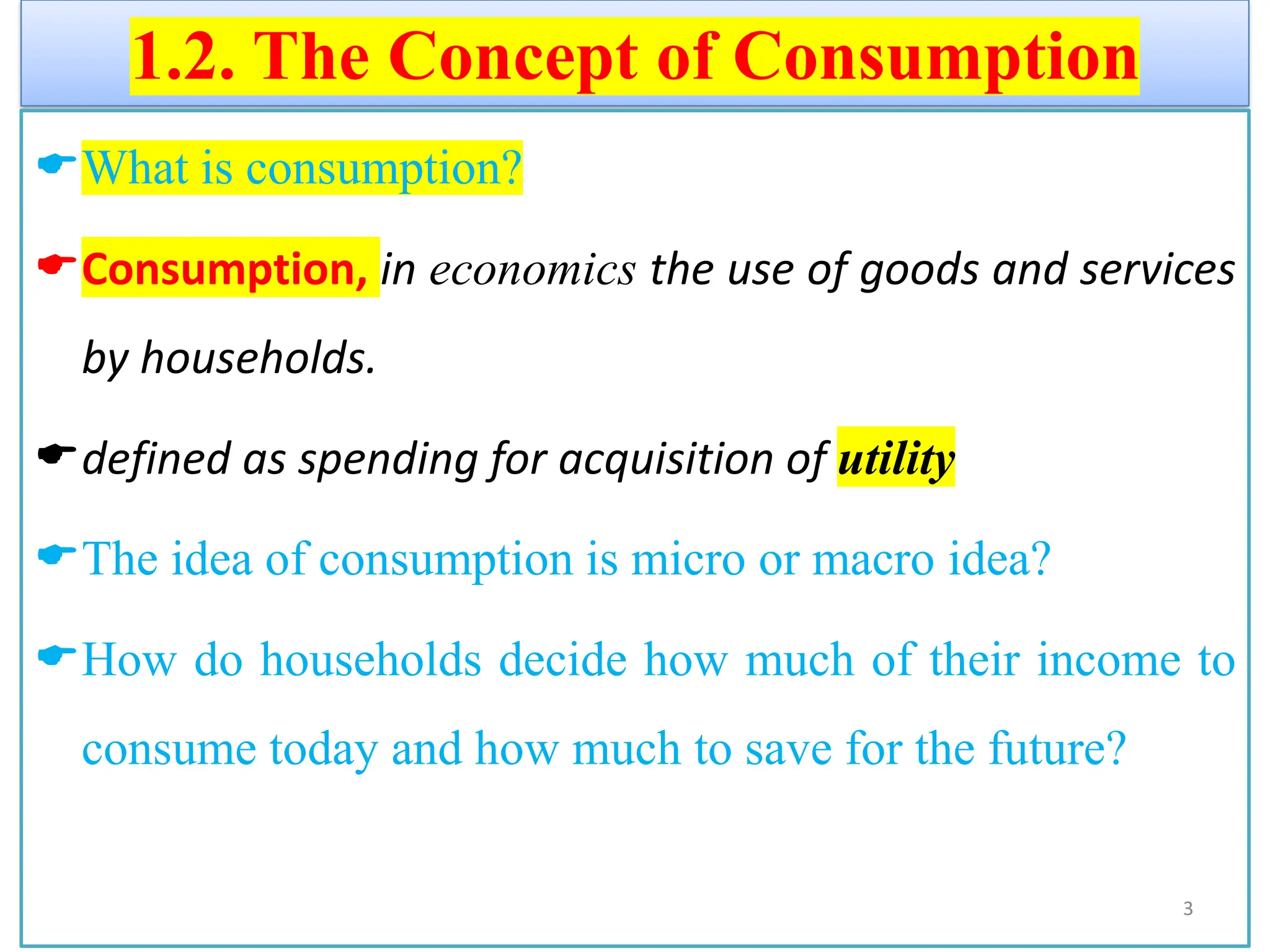
3. 1.2. The Concept of Consumption
What is consumption?
Consumption, in economics the use of goods and services
by households.
defined as spending for acquisition of utility
The idea of consumption is micro or macro idea?
How do households decide how much of their income to
consume today and how much to save for the future?
3

4. Cont’d …
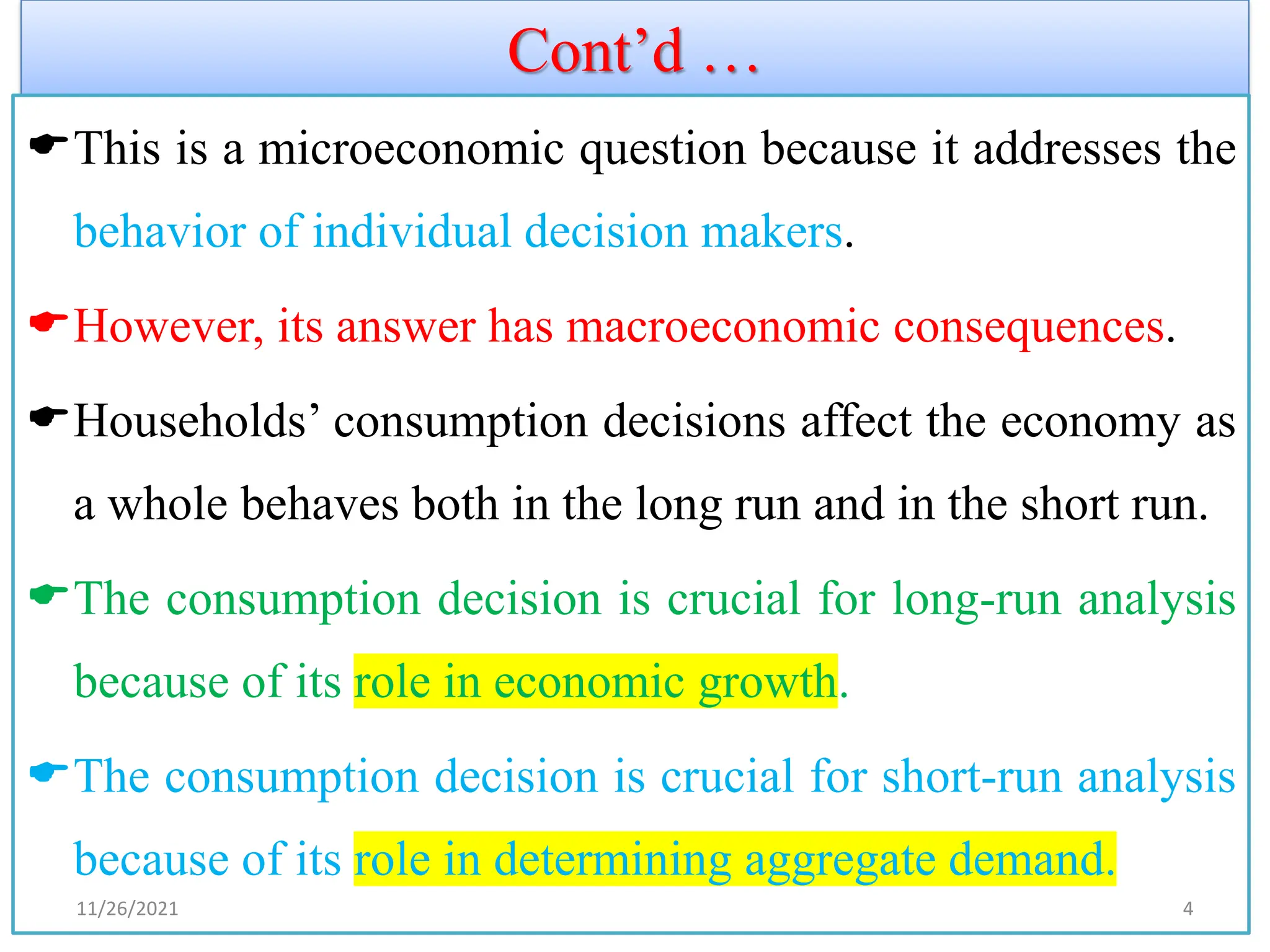
This is a microeconomic question because it addresses the
behavior of individual decision makers.
However, its answer has macroeconomic consequences.
Households’ consumption decisions affect the economy as
a whole behaves both in the long run and in the short run.
The consumption decision is crucial for long-run analysis
because of its role in economic growth.
The consumption decision is crucial for short-run analysis
because of its role in determining aggregate demand.
11/26/2021 4

5. Cont’d …
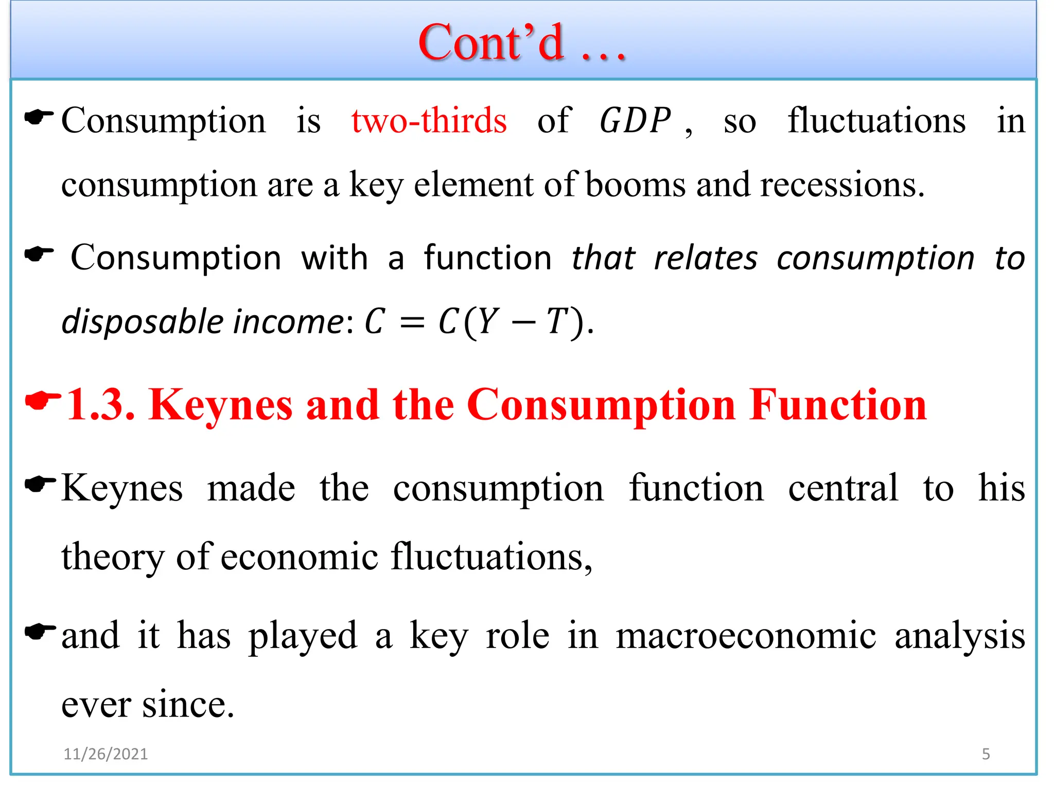
Consumption is two-thirds of 𝐺𝐷𝑃 , so fluctuations in
consumption are a key element of booms and recessions.
 Consumption with a function that relates consumption to
disposable income: 𝐶 = 𝐶(𝑌 − 𝑇).
1.3. Keynes and the Consumption Function
Keynes made the consumption function central to his
theory of economic fluctuations,
and it has played a key role in macroeconomic analysis
ever since.
11/26/2021 5

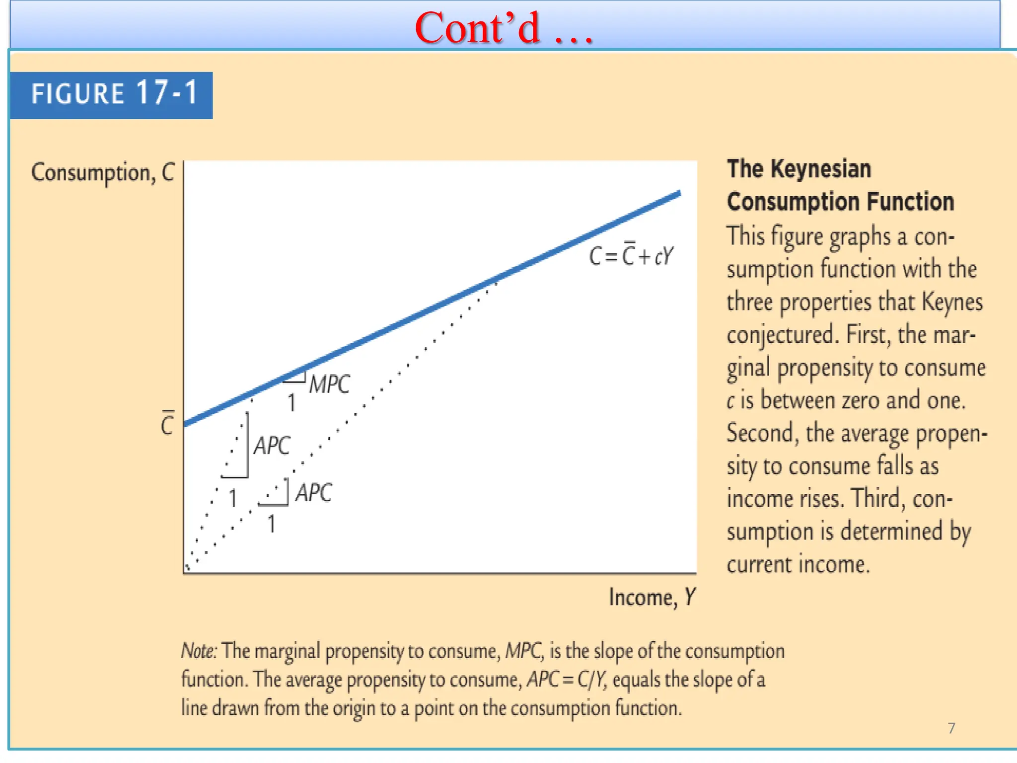
6. Keynes’s Conjectures
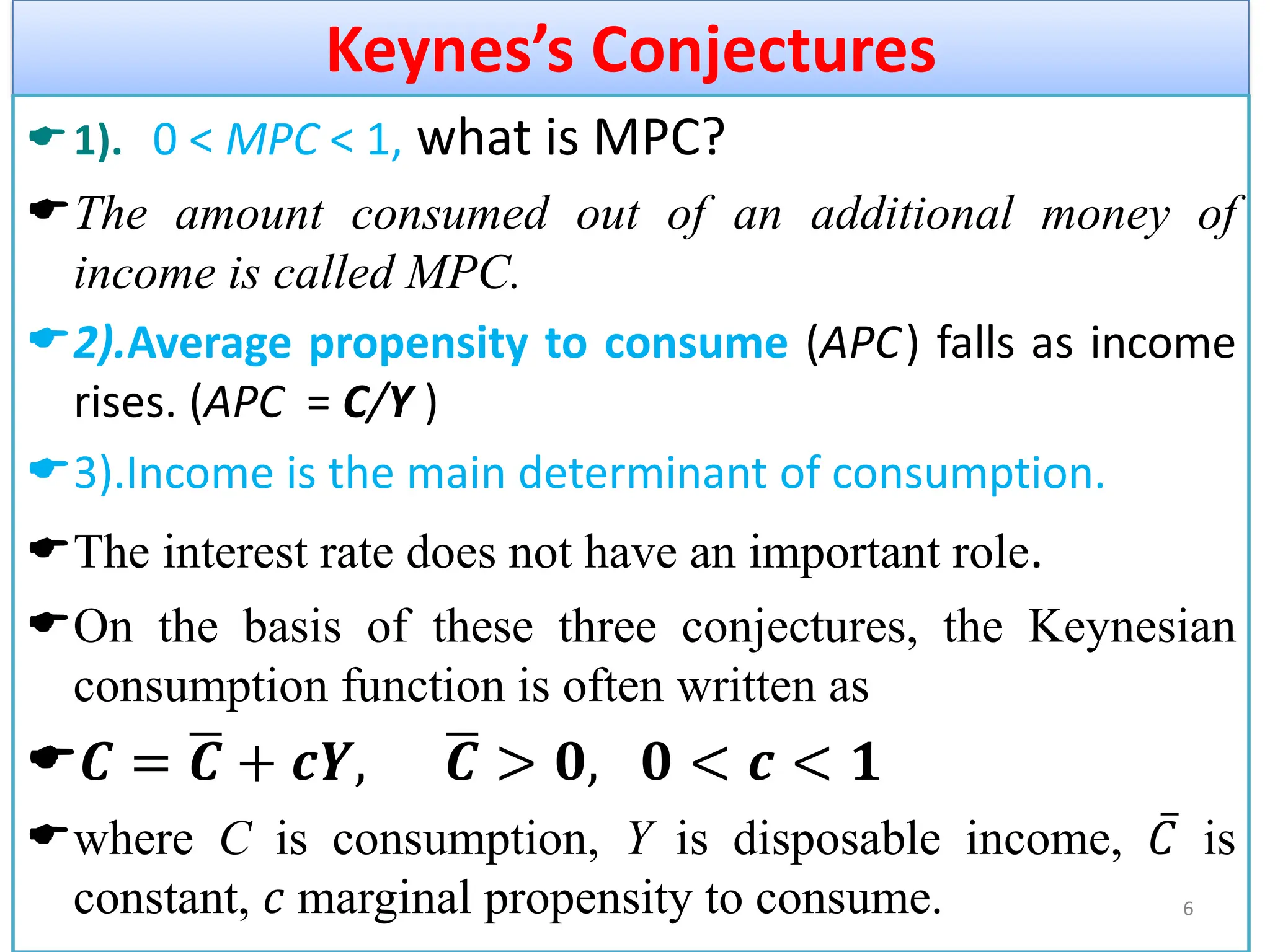
1). 0 < MPC < 1, what is MPC?
The amount consumed out of an additional money of
income is called MPC.
2).Average propensity to consume (APC) falls as income
rises. (APC = C/Y )
3).Income is the main determinant of consumption.
The interest rate does not have an important role.
On the basis of these three conjectures, the Keynesian
consumption function is often written as
𝑪 = ഥ
𝑪 + 𝒄𝒀, ഥ
𝑪 > 𝟎, 𝟎 < 𝒄 < 𝟏
where C is consumption, Y is disposable income, ҧ
𝐶 is
constant, 𝑐 marginal propensity to consume. 6

7. Cont’d …
7

8. The Early Empirical Successes
Soon after Keynes proposed the consumption function,
economists began collecting and examining data to test his
conjectures.
The earliest studies indicated that the Keynesian
consumption function is a good approximation of how
consumers behave.
In some of these studies, researchers surveyed households
and collected data on consumption and income.
They found that households with higher income consumed
more, which confirms that the marginal propensity to
consume is greater than zero.
11/26/2021 8

9. Cont’d …
They also found that households with higher
income saved more, which confirms that the
marginal propensity to consume is less than one.
In addition, these researchers found that higher-
income households saved a larger fraction of their
income, which confirms that APC falls as income
rises.
Thus, these data verified Keynes’s conjectures about the
marginal and average propensities to consume.
In other studies, researchers examined aggregate data on
consumption and income for the period between the
two world wars (i.e., short-time series data).
11/26/2021

10. Cont’d …
These data also supported the Keynesian consumption
function.
In years when income was unusually low, such as during the
depths of the Great Depression, both consumption and saving
were low, indicating that the MPC is between zero and one.
In addition, , during those years of low income, the ratio of
consumption to income was high, confirming Keynes’s second
conjecture that is APC fail.
Thus, the data also confirmed Keynes’s third conjecture that
income is the primary determinant of how much people choose
to consume. 10

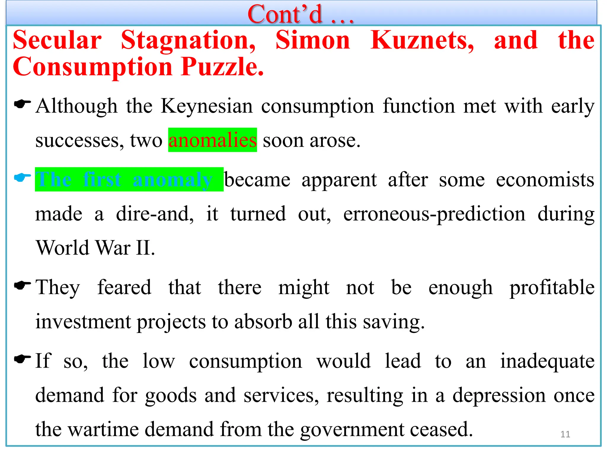
11. Cont’d …
Secular Stagnation, Simon Kuznets, and the
Consumption Puzzle.
Although the Keynesian consumption function met with early
successes, two anomalies soon arose.
The first anomaly became apparent after some economists
made a dire-and, it turned out, erroneous-prediction during
World War II.
They feared that there might not be enough profitable
investment projects to absorb all this saving.
If so, the low consumption would lead to an inadequate
demand for goods and services, resulting in a depression once
the wartime demand from the government ceased. 11

12. Cont’d …
 In other words, on the basis of the Keynesian consumption function,
these economists predicted that the economy would experience what
they called secular stagnation-a long depression of indefinite
duration-unless fiscal policy was used to expand aggregate demand.
 Fortunately for the economy, but unfortunately for the Keynesian
consumption function, the end of World War II did not throw the
country into another depression.
 Although incomes were much higher after the war than before, these
higher incomes did not lead to large increases in the rate of saving.
 Keynes’s conjecture that the average propensity to consume would
fall as income rose appeared not to hold.
12

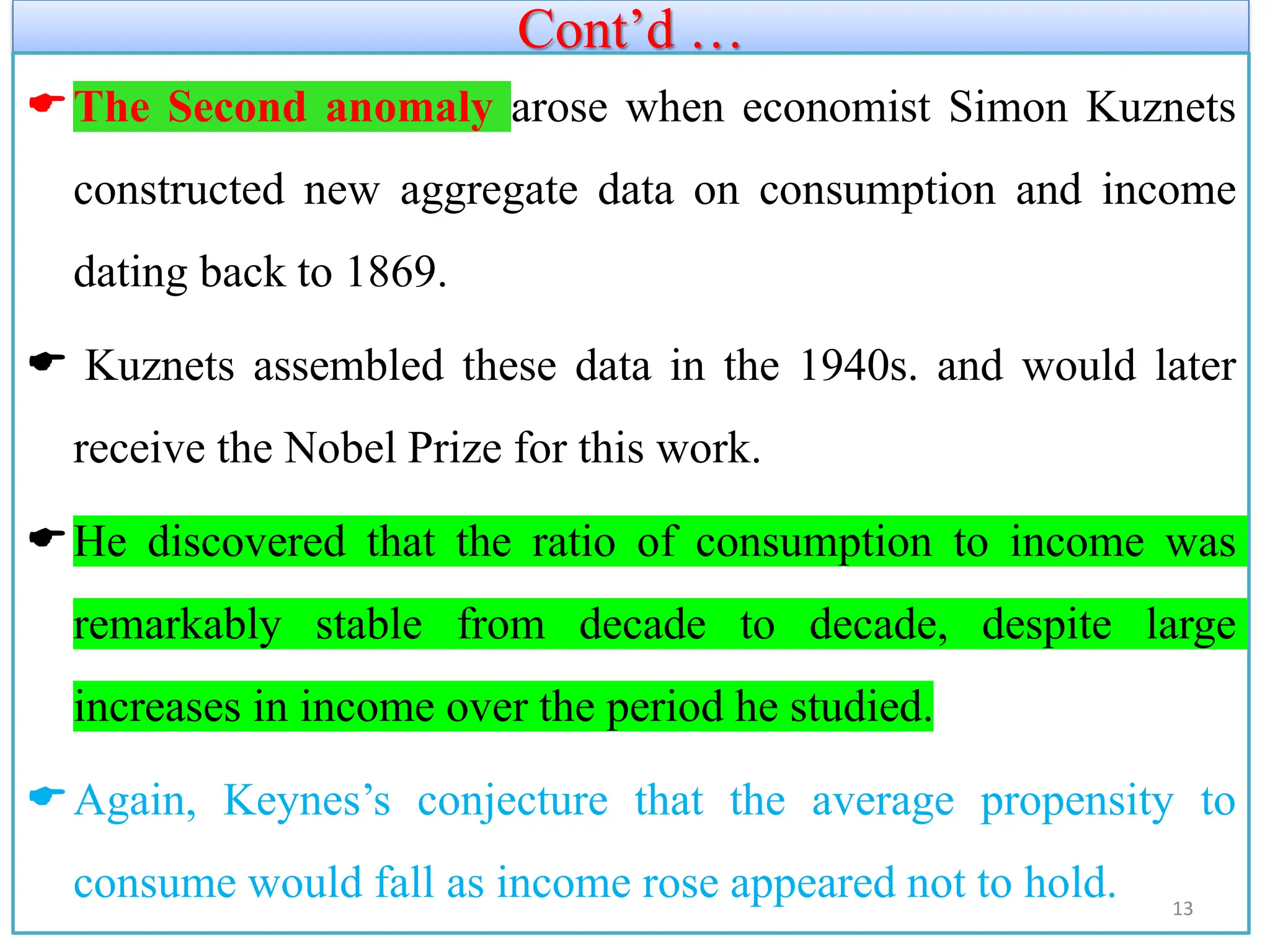
13. Cont’d …
The Second anomaly arose when economist Simon Kuznets
constructed new aggregate data on consumption and income
dating back to 1869.
 Kuznets assembled these data in the 1940s. and would later
receive the Nobel Prize for this work.
He discovered that the ratio of consumption to income was
remarkably stable from decade to decade, despite large
increases in income over the period he studied.
Again, Keynes’s conjecture that the average propensity to
consume would fall as income rose appeared not to hold. 13

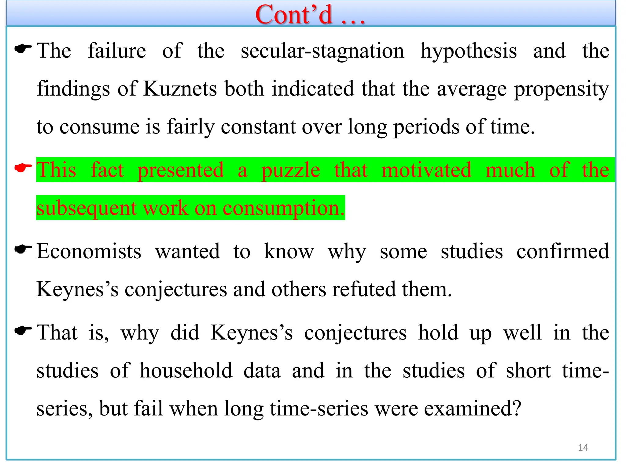
14. Cont’d …
The failure of the secular-stagnation hypothesis and the
findings of Kuznets both indicated that the average propensity
to consume is fairly constant over long periods of time.
This fact presented a puzzle that motivated much of the
subsequent work on consumption.
Economists wanted to know why some studies confirmed
Keynes’s conjectures and others refuted them.
That is, why did Keynes’s conjectures hold up well in the
studies of household data and in the studies of short time-
series, but fail when long time-series were examined?
14

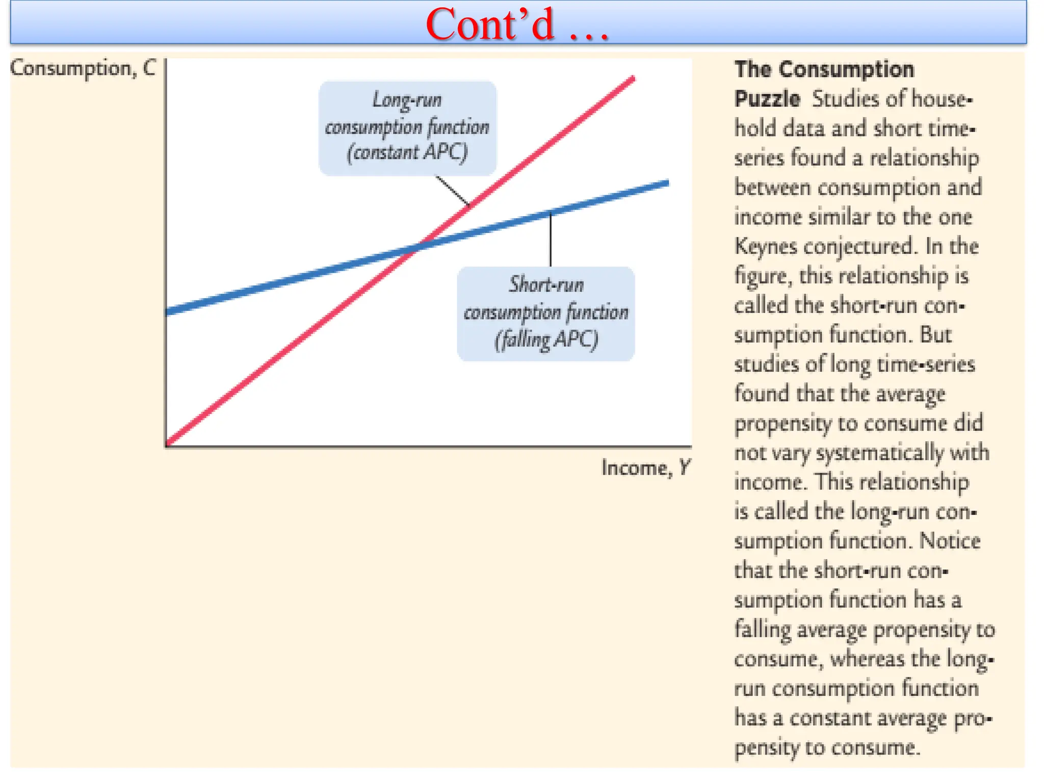
15. Cont’d …
Figure 1-2 illustrates the puzzle. The evidence suggested that
there were two consumption functions. For the household data
or for the short time-series, the Keynesian consumption
function appeared to work well.
Yet for the long time-series, the consumption function
appeared to have a constant average propensity to consume.
11/26/2021 15

16. Cont’d …
11/26/2021 16

17. 1.4 Fisher and Intertemporal Choice
The consumption function introduced by Keynes relates
current consumption to current income.
This relationship, however, is incomplete at best.
When people decide how much to consume and how
much to save, they consider both the present and the
future.
The more consumption they enjoy today, the less they will
be able to enjoy tomorrow.
17

18. Cont’d …
The economist Irving Fisher developed the model with
which economists analyze how rational, forward-looking
consumers make intertemporal choices-
that is, choices involving different periods of time.
Fisher’s model illuminates the constraints consumers face,
the preferences they have, and how these constraints and
preferences together determine their choices about
consumption and saving.
18

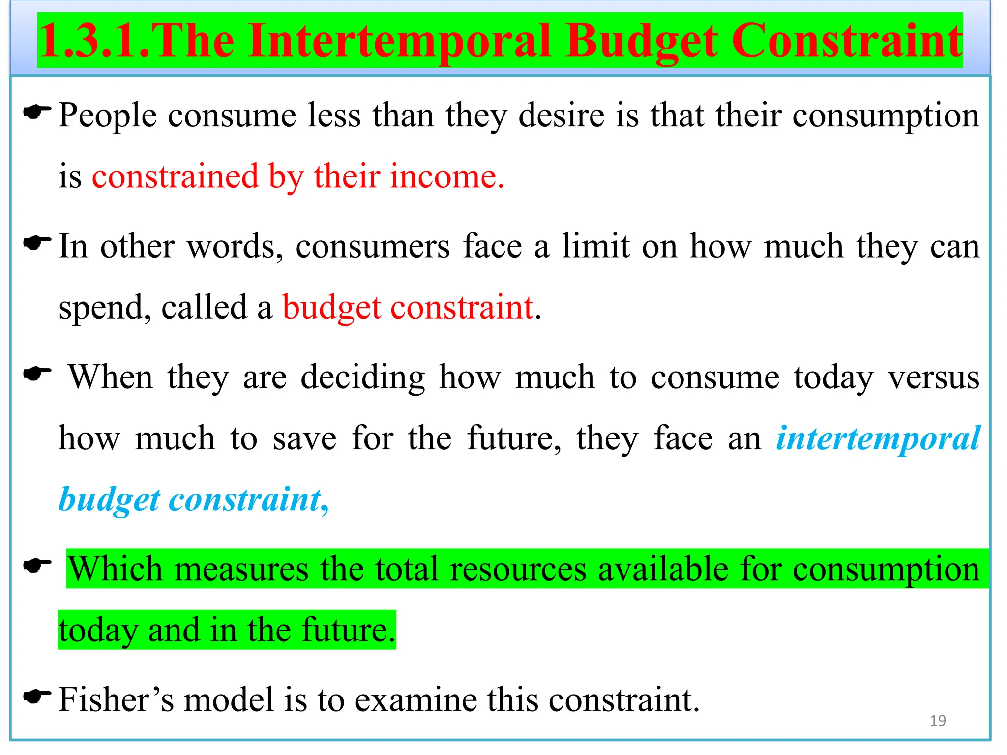
19. 1.3.1.The Intertemporal Budget Constraint
People consume less than they desire is that their consumption
is constrained by their income.
In other words, consumers face a limit on how much they can
spend, called a budget constraint.
 When they are deciding how much to consume today versus
how much to save for the future, they face an intertemporal
budget constraint,
 Which measures the total resources available for consumption
today and in the future.
Fisher’s model is to examine this constraint. 19

20. Cont’d …
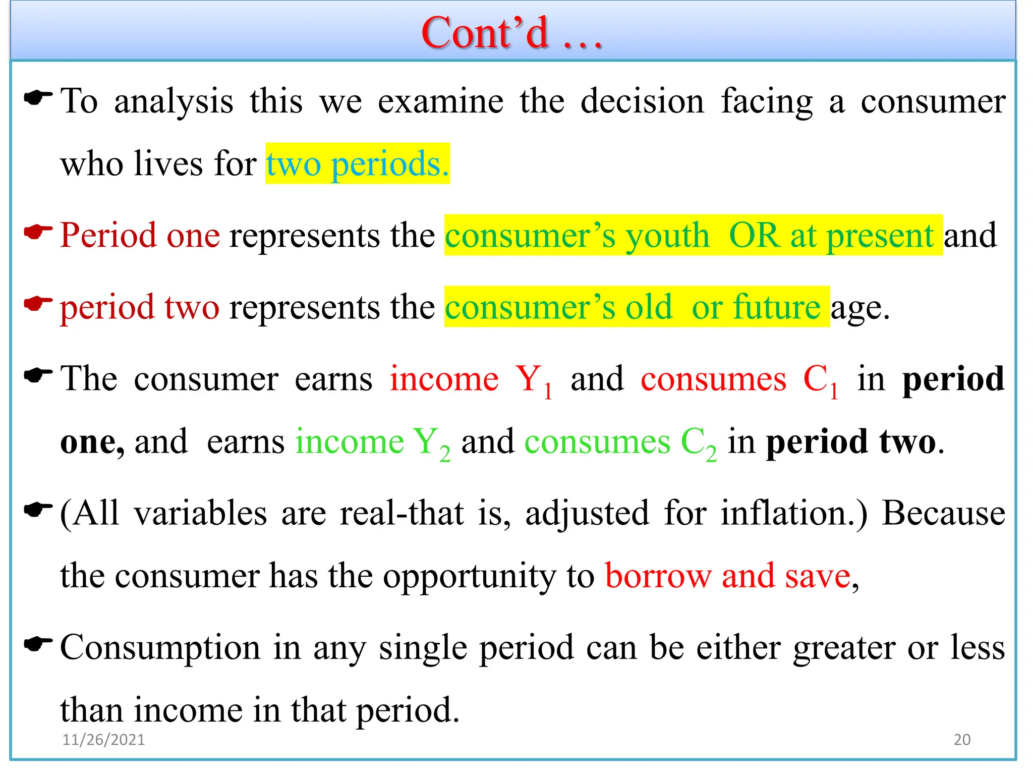
To analysis this we examine the decision facing a consumer
who lives for two periods.
Period one represents the consumer’s youth OR at present and
period two represents the consumer’s old or future age.
The consumer earns income Y1 and consumes C1 in period
one, and earns income Y2 and consumes C2 in period two.
(All variables are real-that is, adjusted for inflation.) Because
the consumer has the opportunity to borrow and save,
Consumption in any single period can be either greater or less
than income in that period.
11/26/2021 20

21. Cont’d …
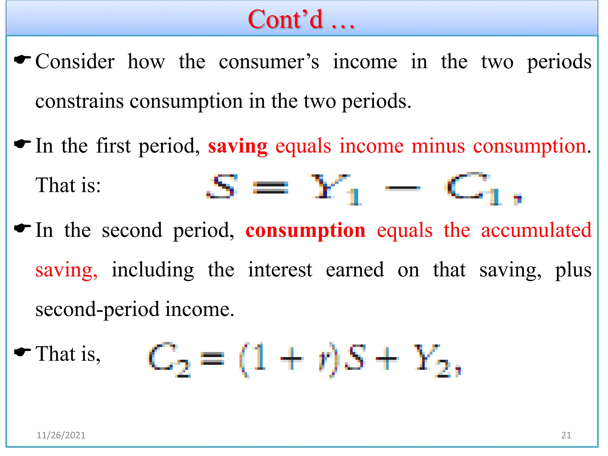
Consider how the consumer’s income in the two periods
constrains consumption in the two periods.
In the first period, saving equals income minus consumption.
That is:
In the second period, consumption equals the accumulated
saving, including the interest earned on that saving, plus
second-period income.
That is,
11/26/2021 21

22. Cont’d …
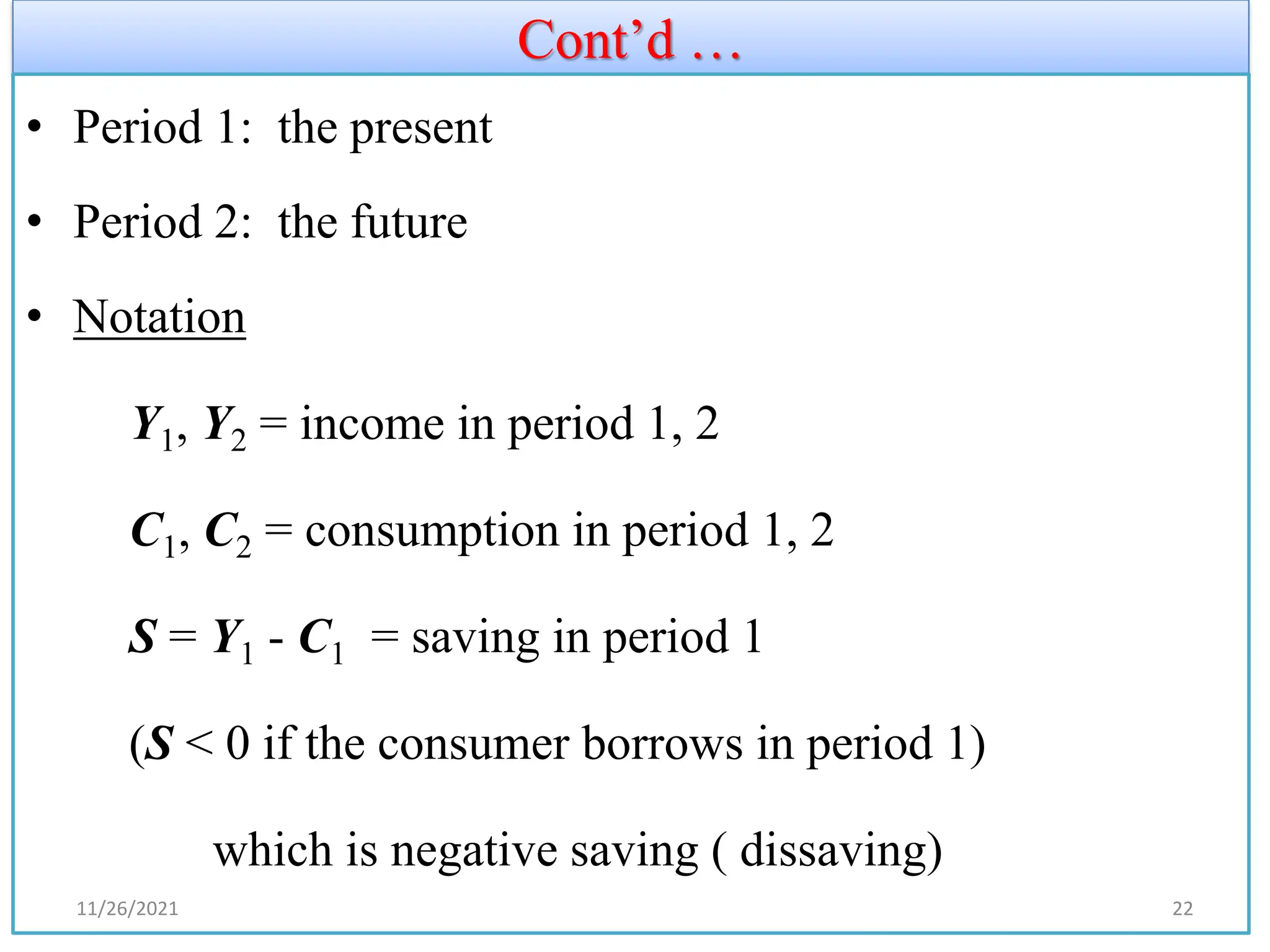
• Period 1: the present
• Period 2: the future
• Notation
Y1, Y2 = income in period 1, 2
C1, C2 = consumption in period 1, 2
S = Y1 - C1 = saving in period 1
(S < 0 if the consumer borrows in period 1)
which is negative saving ( dissaving)
11/26/2021 22

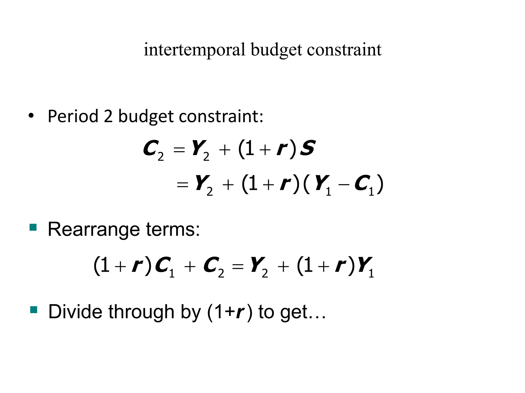
23. intertemporal budget constraint
• Period 2 budget constraint:
2 2 (1 )
C Y r S
= + +
2 1 1
(1 )( )
Y r Y C
= + + −
▪ Rearrange terms:
1 2 2 1
(1 ) (1 )
r C C Y r Y
+ + = + +
▪ Divide through by (1+r) to get…

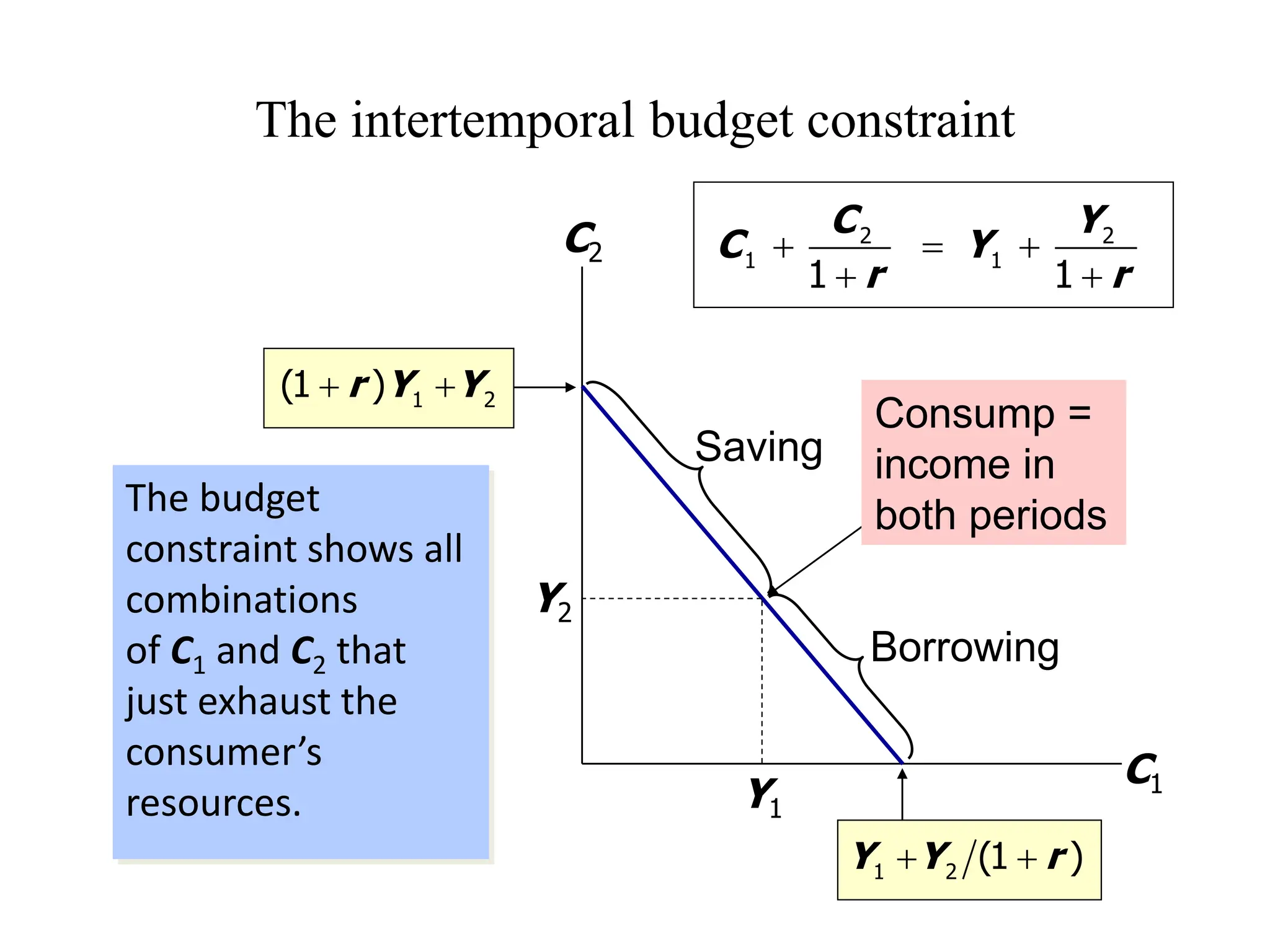
24. The intertemporal budget constraint
2 2
1 1
1 1
C Y
C Y
r r
+ = +
+ +
present value of
lifetime consumption
present value of
lifetime income

25. Cont’d …
11/26/2021 25

26. The intertemporal budget constraint
The budget
constraint shows all
combinations
of C1 and C2 that
just exhaust the
consumer’s
resources.
C1
C2
1 2 (1 )
Y Y r
+ +
1 2
(1 )
r Y Y
+ +
Y1
Y2
Borrowing
Saving
Consump =
income in
both periods
2 2
1 1
1 1
C Y
C Y
r r
+ = +
+ +

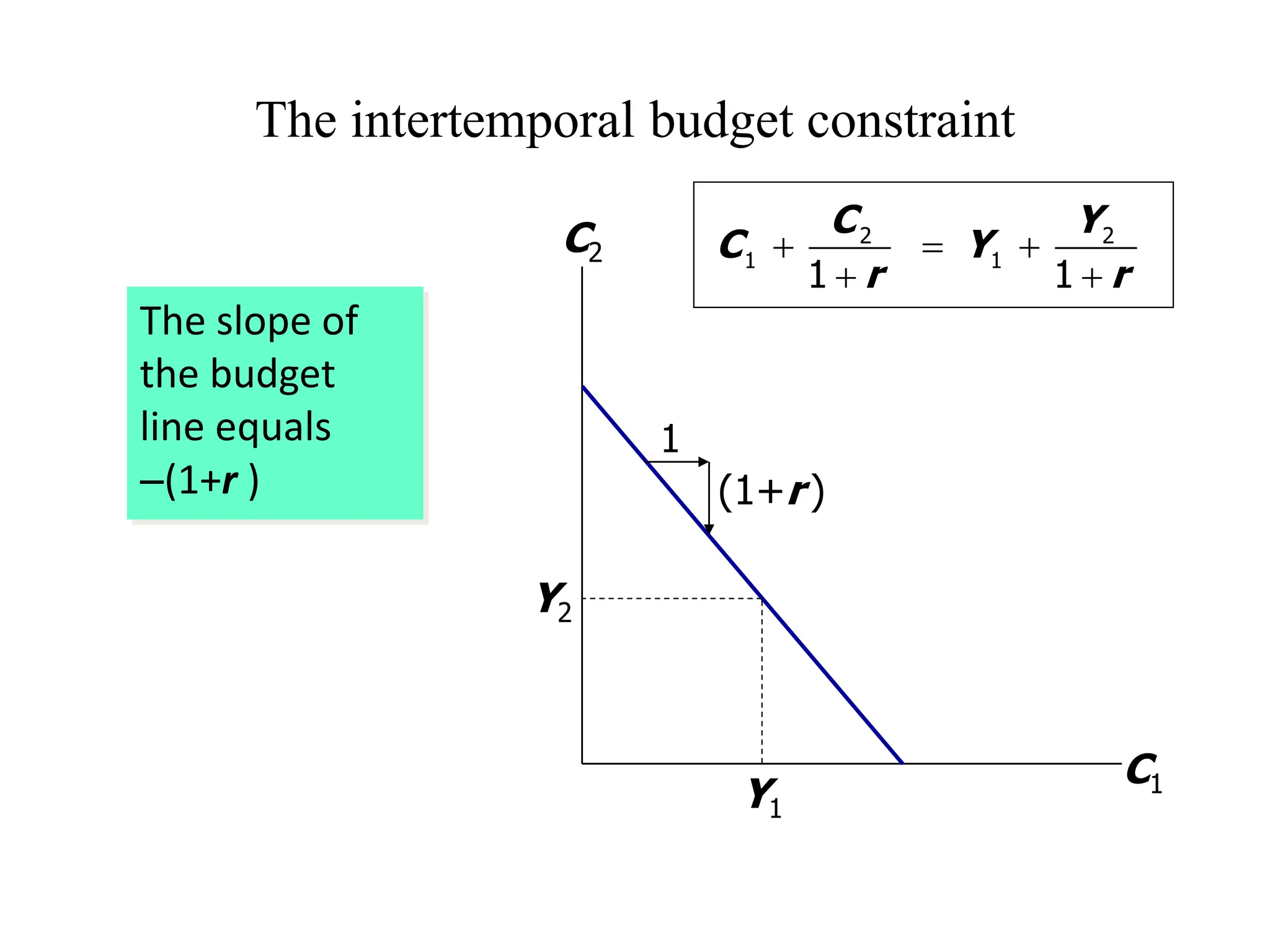
27. The intertemporal budget constraint
The slope of
the budget
line equals
−(1+r )
C1
C2
Y1
Y2
1
(1+r )
2 2
1 1
1 1
C Y
C Y
r r
+ = +
+ +

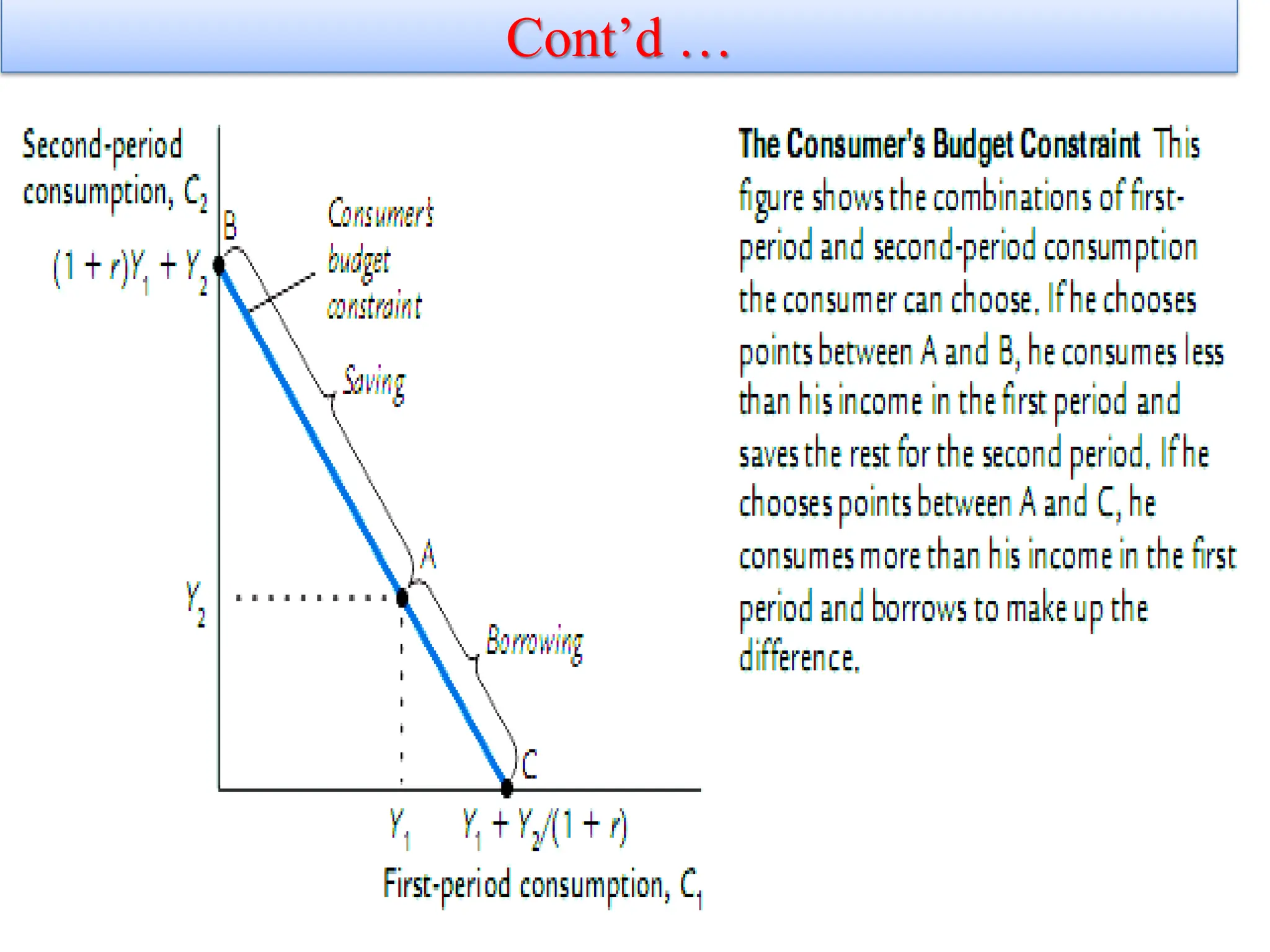
28. Cont’d …
At point A, the consumer consumes exactly his income in each
period (C1 = Y1 and C2 = Y2), so there is neither saving nor
borrowing between the two periods.
At point B, the consumer consumes nothing in the first period
(C1=0) and saves all income, so second-period consumption C2
is (1 +r) Y1 +Y2.
 At point C, the consumer plans to consume nothing in the
second period (C2=0) and borrows as much as possible against
second-period income, so first-period consumption C1 is Y1 +
Y2 /(1 + r).

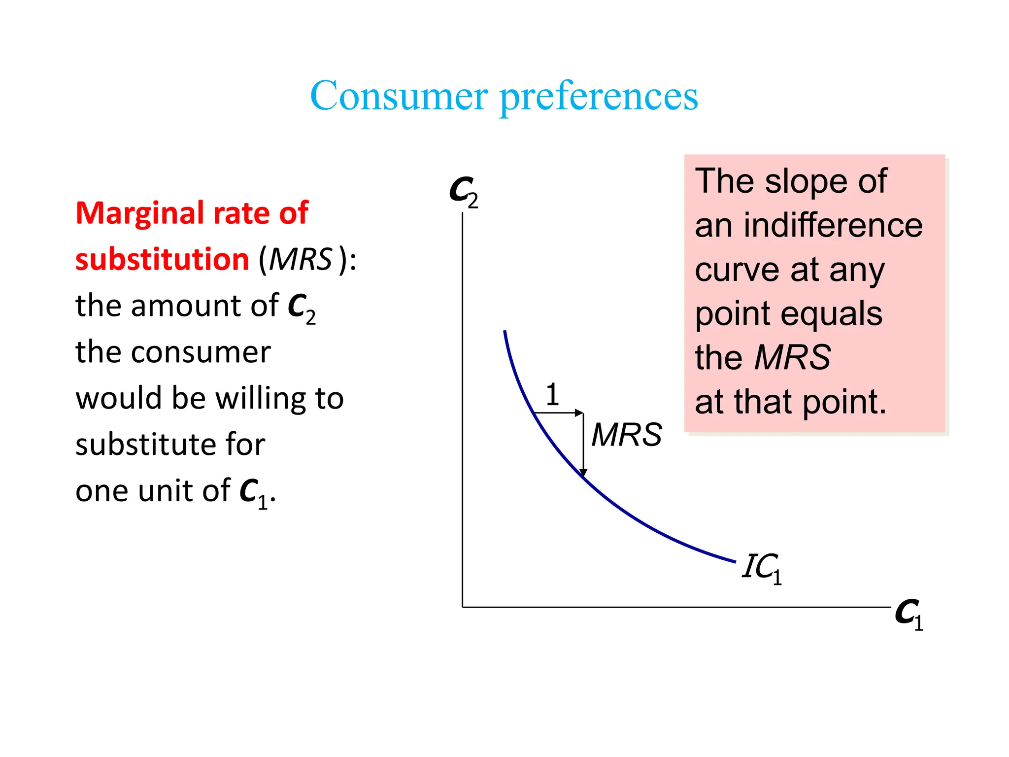
29. 1.3.2.Consumer Preferences
The consumer’s preferences regarding consumption in the
two periods can be represented by indifference curves.
 An indifference curve shows the combinations of first-
period and second-period consumption that make the
consumer equally happy.
The slope is the marginal rate of substitution between
first-period consumption and second-period consumption.
It tells us the rate at which the consumer is willing to
substitute second-period consumption for first-period
consumption.
11/26/2021 29

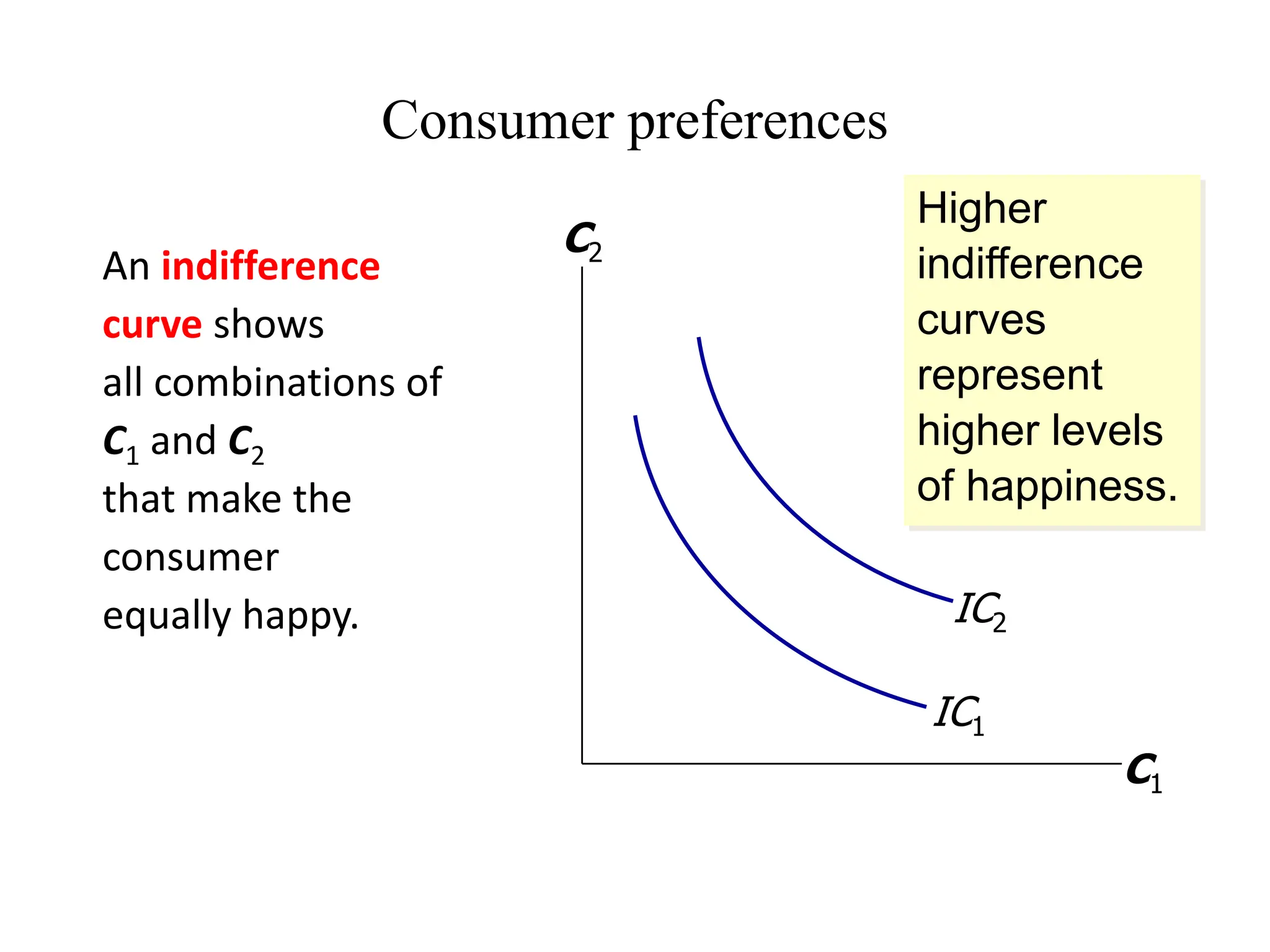
30. Consumer preferences
An indifference
curve shows
all combinations of
C1 and C2
that make the
consumer
equally happy.
C1
C2
IC1
IC2
Higher
indifference
curves
represent
higher levels
of happiness.

31. Consumer preferences
Marginal rate of
substitution (MRS):
the amount of C2
the consumer
would be willing to
substitute for
one unit of C1.
C1
C2
IC1
The slope of
an indifference
curve at any
point equals
the MRS
at that point.
1
MRS

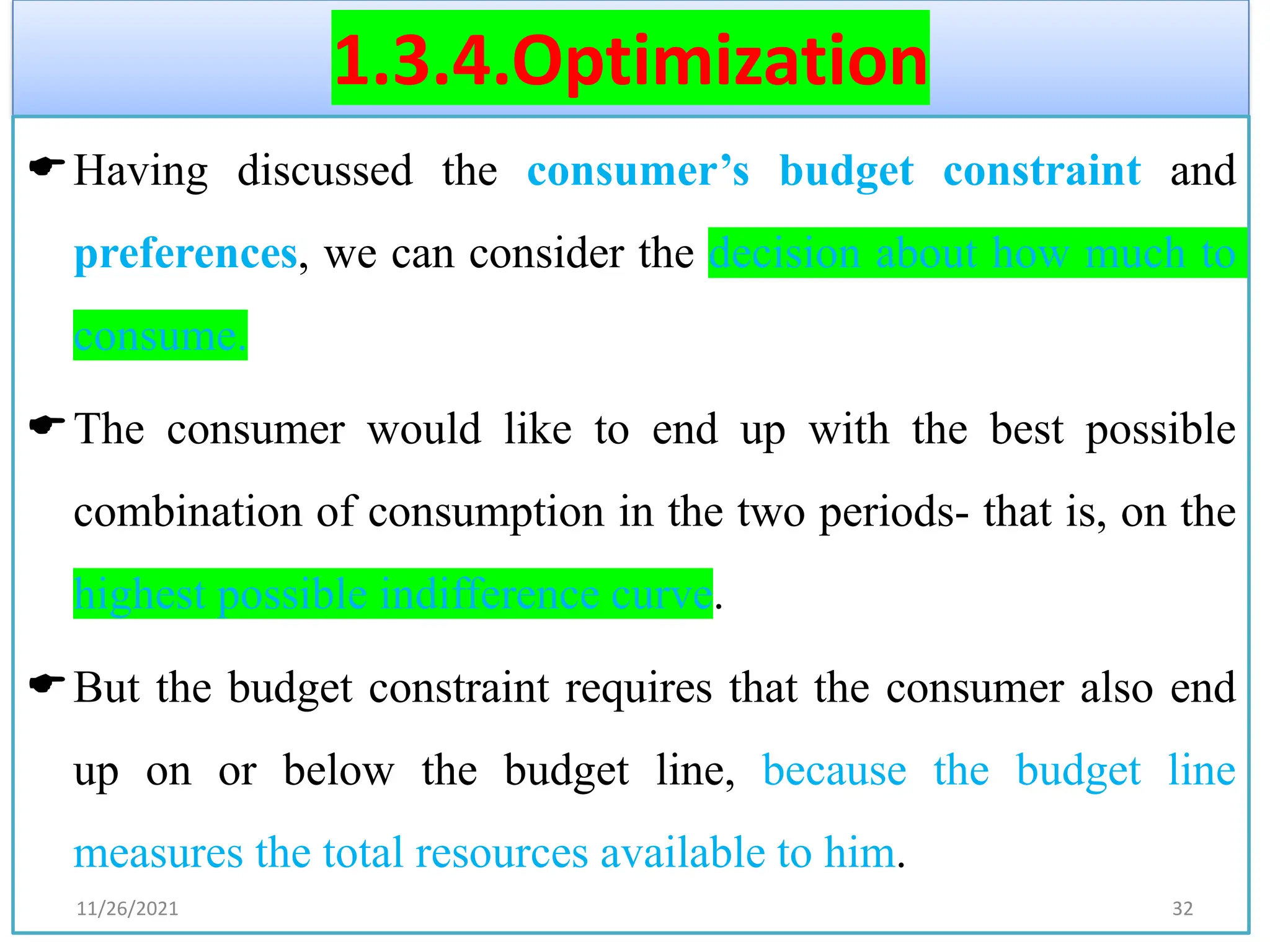
32. 1.3.4.Optimization
Having discussed the consumer’s budget constraint and
preferences, we can consider the decision about how much to
consume.
The consumer would like to end up with the best possible
combination of consumption in the two periods- that is, on the
highest possible indifference curve.
But the budget constraint requires that the consumer also end
up on or below the budget line, because the budget line
measures the total resources available to him.
11/26/2021 32

33. Inter Temporal Choice (Irving Fisher)
The consumer has to choose C1 and C2 so as to
✓ The optimal solution is at a point where the slope of the
budget line, (1+r) equals the slope of an IC, MRS.
MRS = (1+r)
– The slope of the budget line means to increase C1 by one
unit, the consumer must sacrifice (1+r) units of C2.
– The slope of an indifference curve (MRS) measures the
amount of C2 the consumer would be willing to
substitute for one unit of C1.
2 2
1 1
1 1
C Y
C Y
r r
+ = +
+ +
33

34. Cont’d …
11/26/2021 34

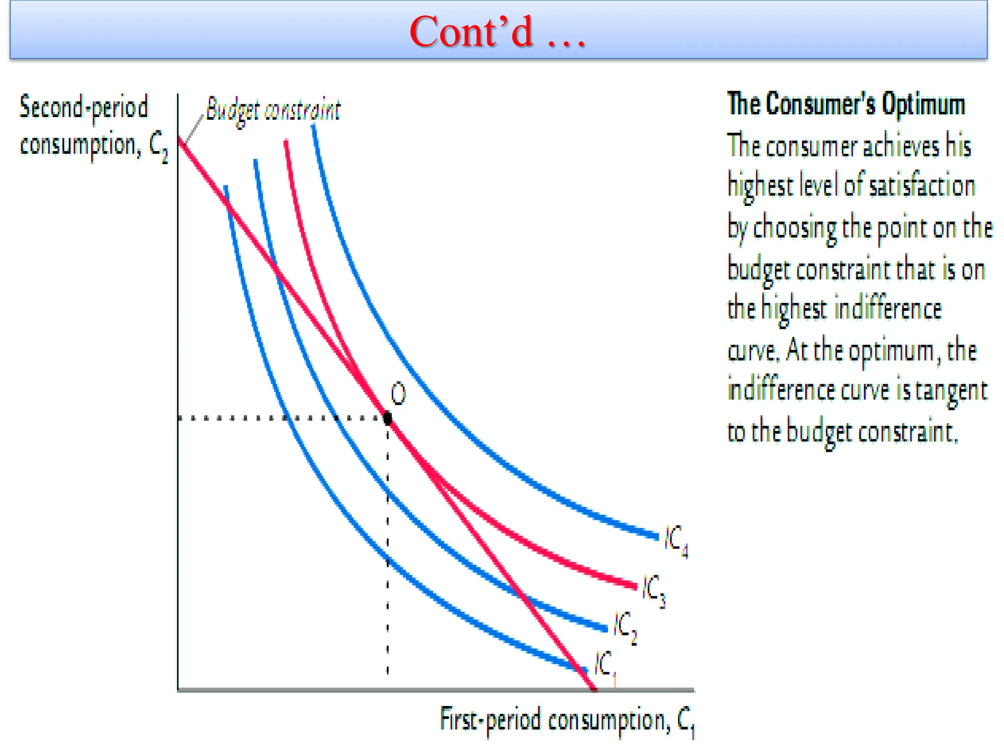
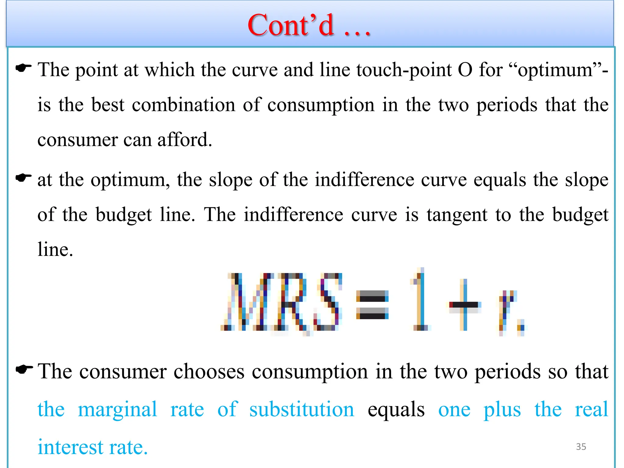
35. Cont’d …
 The point at which the curve and line touch-point O for “optimum”-
is the best combination of consumption in the two periods that the
consumer can afford.
 at the optimum, the slope of the indifference curve equals the slope
of the budget line. The indifference curve is tangent to the budget
line.
The consumer chooses consumption in the two periods so that
the marginal rate of substitution equals one plus the real
interest rate. 35

36. Cont’d …
11/26/2021 36
❖QUESTIONS
❖Abebe obeys the two-period Fisher’s model consumption.
He earns nothing in the first period, and earns 11,000 birr in
the second period. He can borrow or save money at the
interest rate 𝑟. We observe that Abebe consuming 5000 birr
in the first period and 5000 in the second period. What is
the interest rate 𝑟 ?

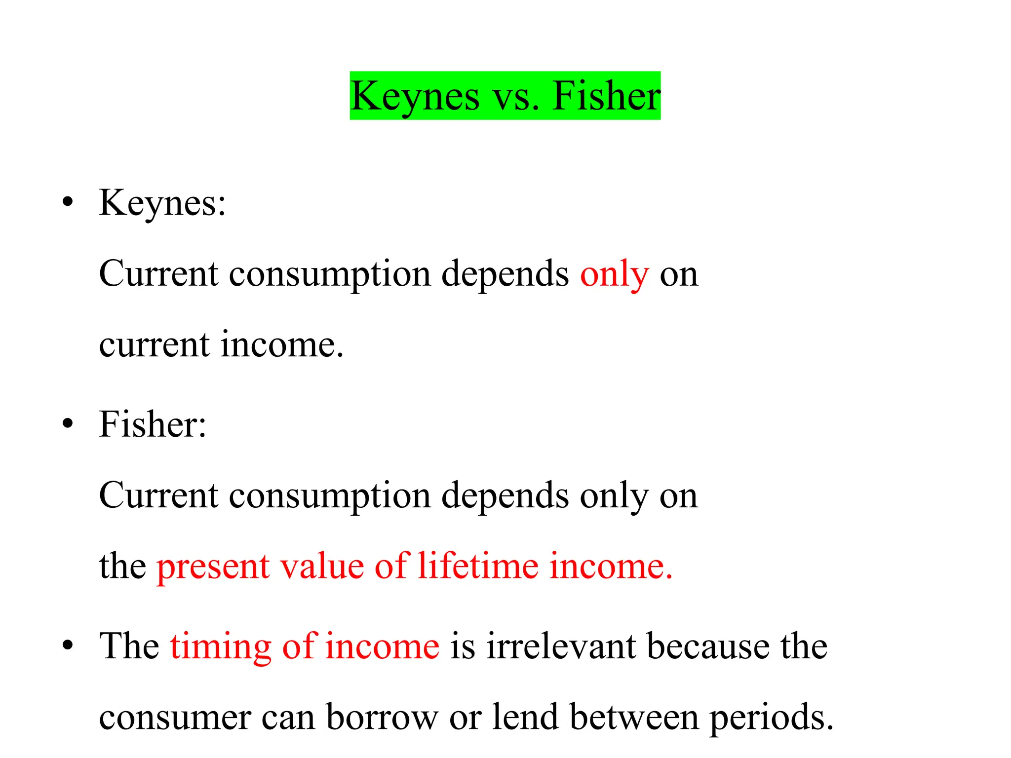
37. Keynes vs. Fisher
• Keynes:
Current consumption depends only on
current income.
• Fisher:
Current consumption depends only on
the present value of lifetime income.
• The timing of income is irrelevant because the
consumer can borrow or lend between periods.

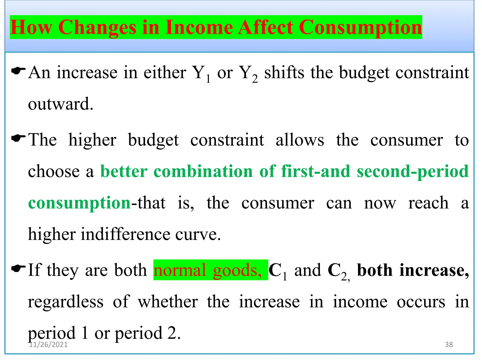
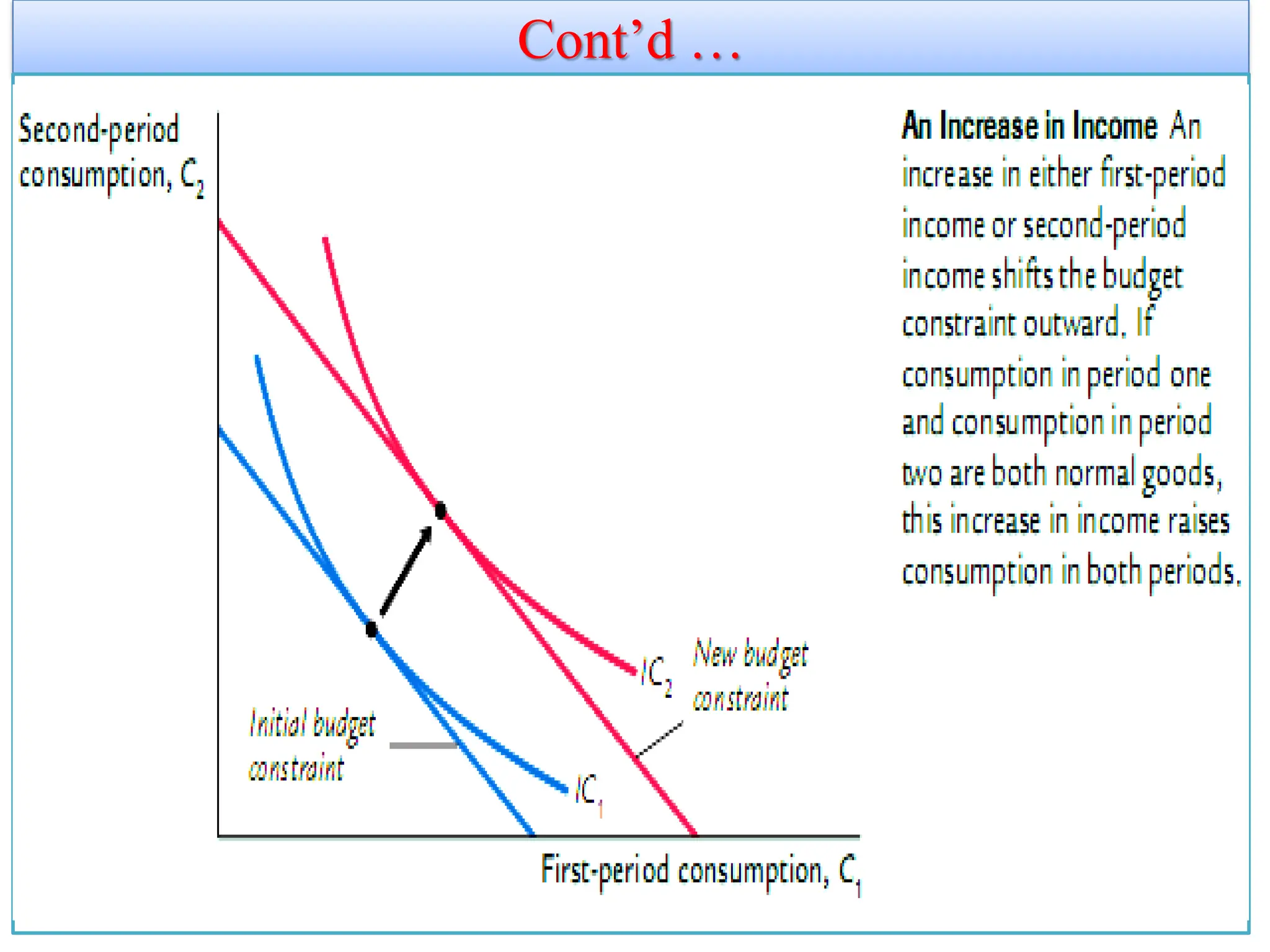
38. How Changes in Income Affect Consumption
An increase in either Y1 or Y2 shifts the budget constraint
outward.
The higher budget constraint allows the consumer to
choose a better combination of first-and second-period
consumption-that is, the consumer can now reach a
higher indifference curve.
If they are both normal goods, C1 and C2, both increase,
regardless of whether the increase in income occurs in
period 1 or period 2.
11/26/2021 38

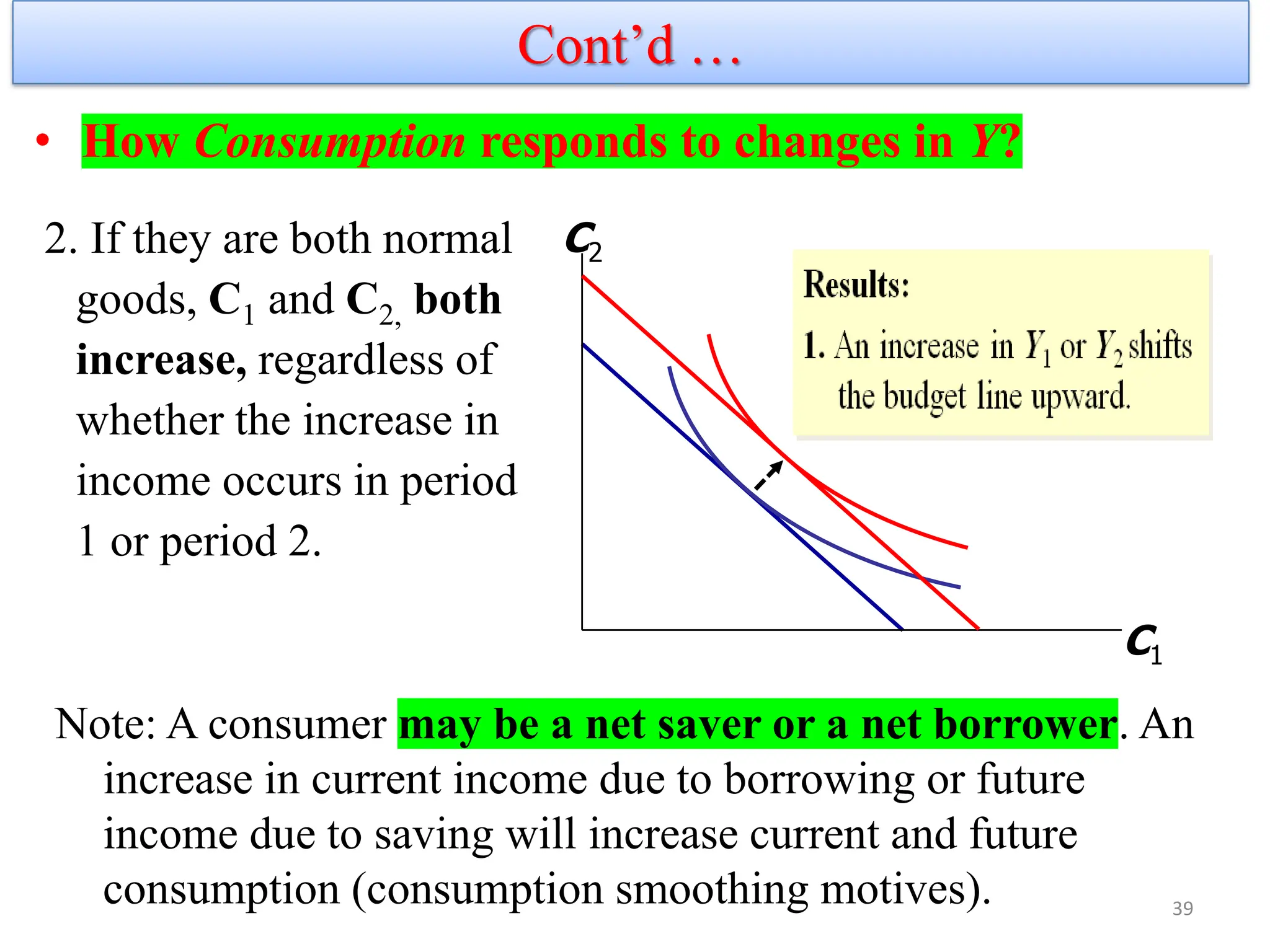
39. • How Consumption responds to changes in Y?
C1
C2
2. If they are both normal
goods, C1 and C2, both
increase, regardless of
whether the increase in
income occurs in period
1 or period 2.
Note: A consumer may be a net saver or a net borrower. An
increase in current income due to borrowing or future
income due to saving will increase current and future
consumption (consumption smoothing motives). 39
Cont’d …

40. Cont’d …
11/26/2021 40

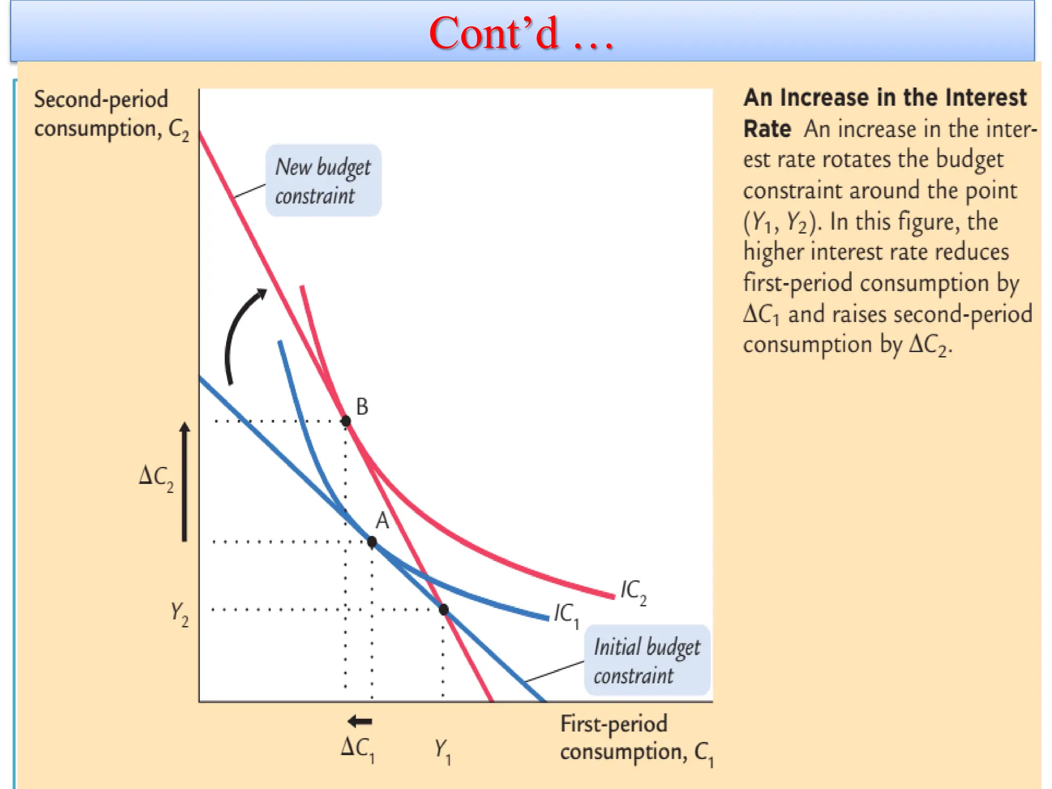
41. Changes in the Real Interest Rate Affect Consumption
There are two cases to consider:
Case 1: the consumer is initially saving and
 Case 2: the consumer is initially borrowing.
Here we discuss the saving case;
an increase in the real interest rate rotates the consumer’s
budget line around the point (Y1, Y2).
Economists decompose the impact of an increase in the real
interest rate on consumption into two effects: an income
effect and a substitution effect.
41

42. Cont’d …
The income effect :If consumer is a saver, the rise in r makes him
better off, which tends to increase consumption in both periods.
How? the change in consumption that results from the
movement to a higher indifference curve.
 Because the consumer is a saver rather than a borrower (as
indicated by the fact that first-period consumption is less than
first-period income).
the increase in the interest rate makes him better off (as
reflected by the movement to a higher indifference curve).
11/26/2021 42

43. Cont’d …
 If consumption in period one and consumption in period two
are both normal goods, the consumer will want to spread this
improvement in his welfare over both periods.
This income effect tends to make the consumer want more
consumption in both periods.
The substitution effect : The rise in r increases opportunity
cost of current consumption, which tends to reduce C1 and
increase C2.
the change in consumption that results from the change in the
relative price of consumption in the two periods. 43

44. Cont’d …
In particular, C2 becomes less expensive relative to C in
period one when the interest rate rises.
That is, because the real interest rate earned on saving is
higher, the consumer must now give up less first-period C
to obtain an extra unit of second-period C.
This substitution effect tends to make the consumer
choose more consumption in period two and less
consumption in period one.
11/26/2021 44

45. Cont’d …
 The consumer’s choice depends on both the income effect and the
substitution effect.
 Both effects act to increase the amount of second-period
consumption.
 hence, we can conclude that an increase in the real interest rate
raises second-period consumption.
 But the two effects have opposite impacts on first-period
consumption, so the increase in the interest rate could either raise
or lower it.
 Hence, depending on the relative size of the income and
substitution effects.
45

46. Cont’d …
11/26/2021 46

47. Cont’d …
If the consumer is a net borrower, The ability to
borrow allows current consumption to exceed current income.
 In essence, when the consumer borrows, he consumes some of
his future income today.
 Constraints on Borrowing
However, for many people borrowing is impossible.
For example, a student wishing to enjoy summer break in
in Langano would probably be unable to finance this
vacation with a bank loan.
11/26/2021 47

48. Cont’d …
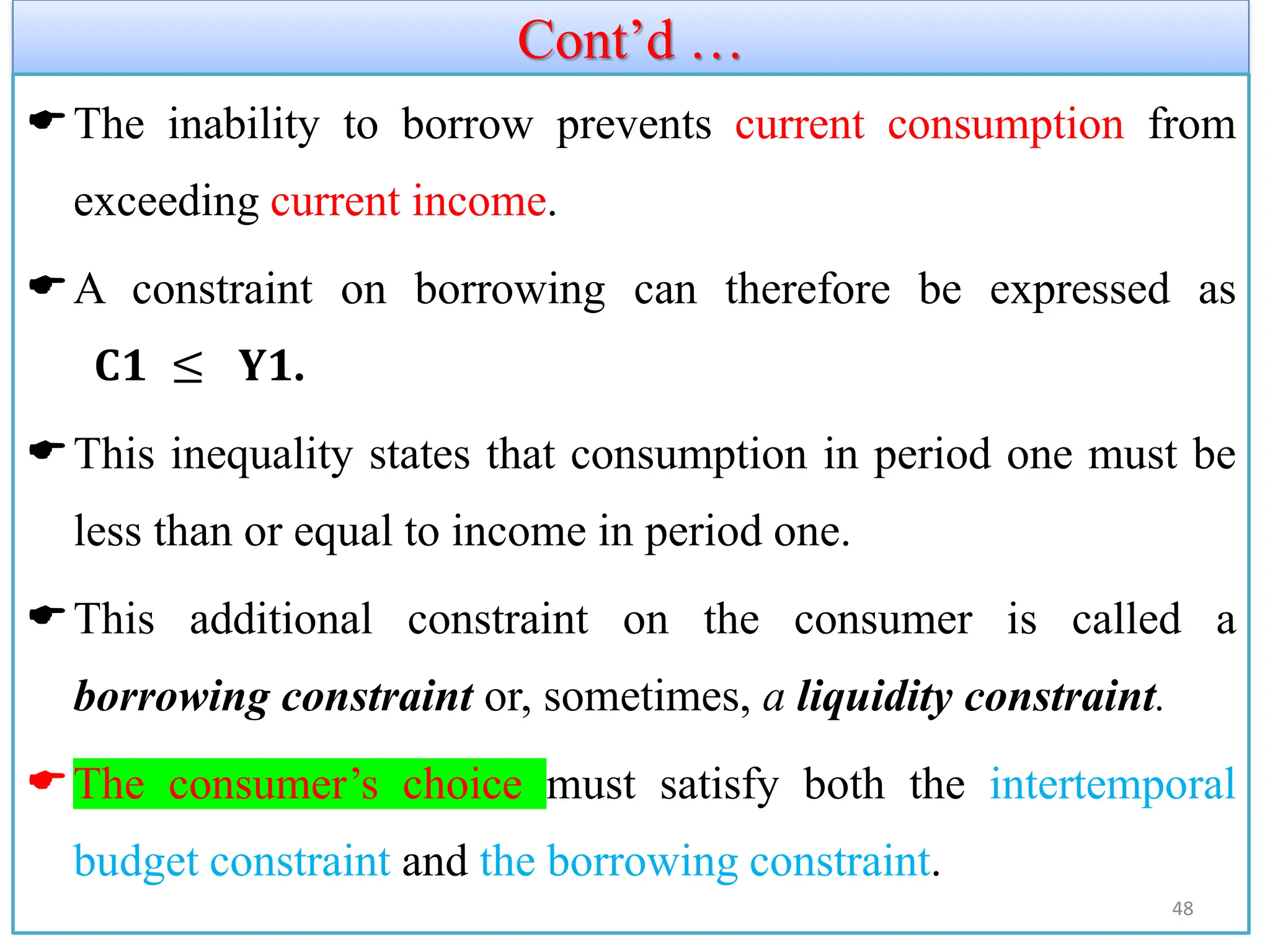
The inability to borrow prevents current consumption from
exceeding current income.
A constraint on borrowing can therefore be expressed as
𝐂𝟏 ≤ 𝐘𝟏.
This inequality states that consumption in period one must be
less than or equal to income in period one.
This additional constraint on the consumer is called a
borrowing constraint or, sometimes, a liquidity constraint.
The consumer’s choice must satisfy both the intertemporal
budget constraint and the borrowing constraint.
48

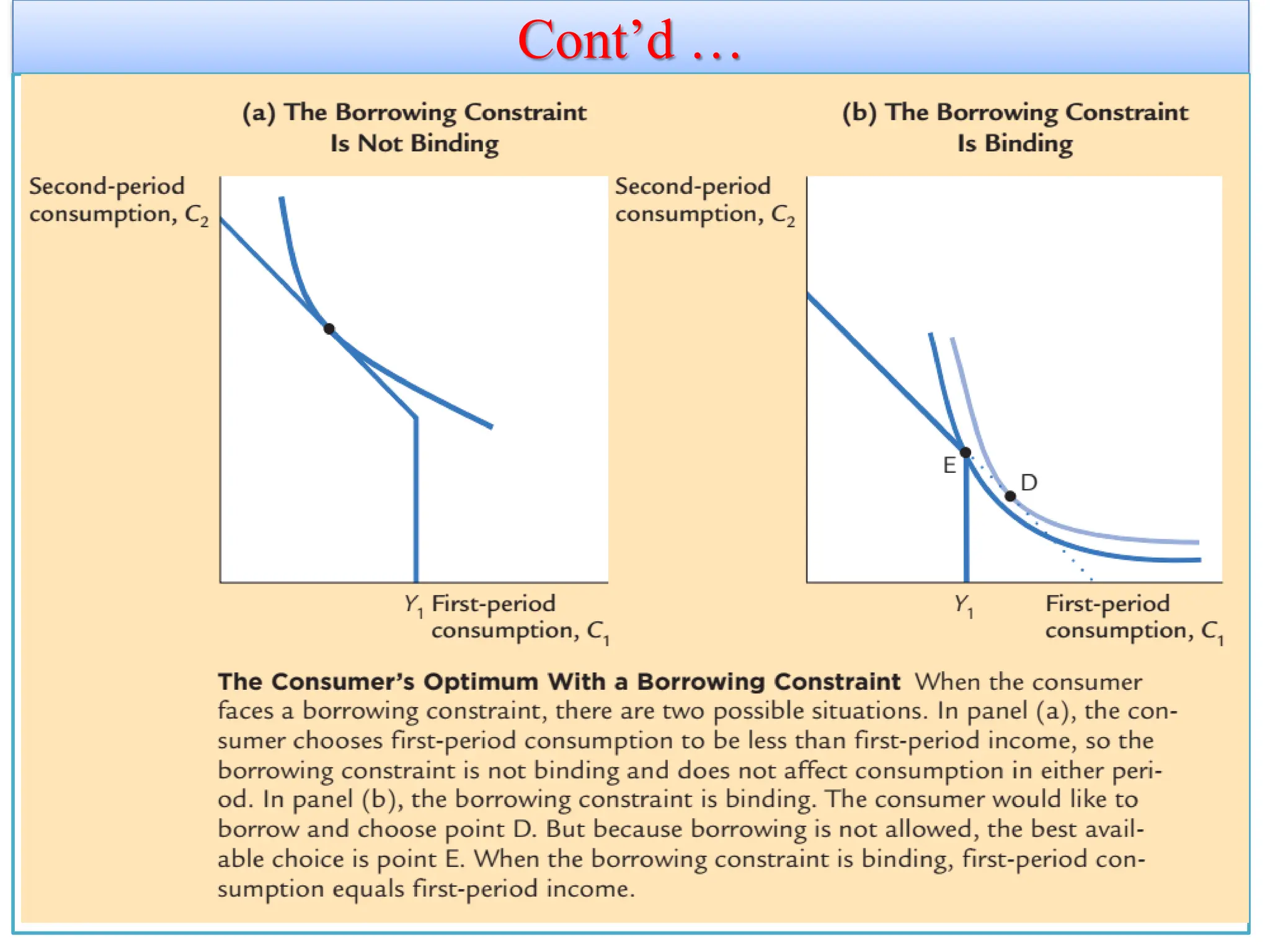
49. Cont’d …
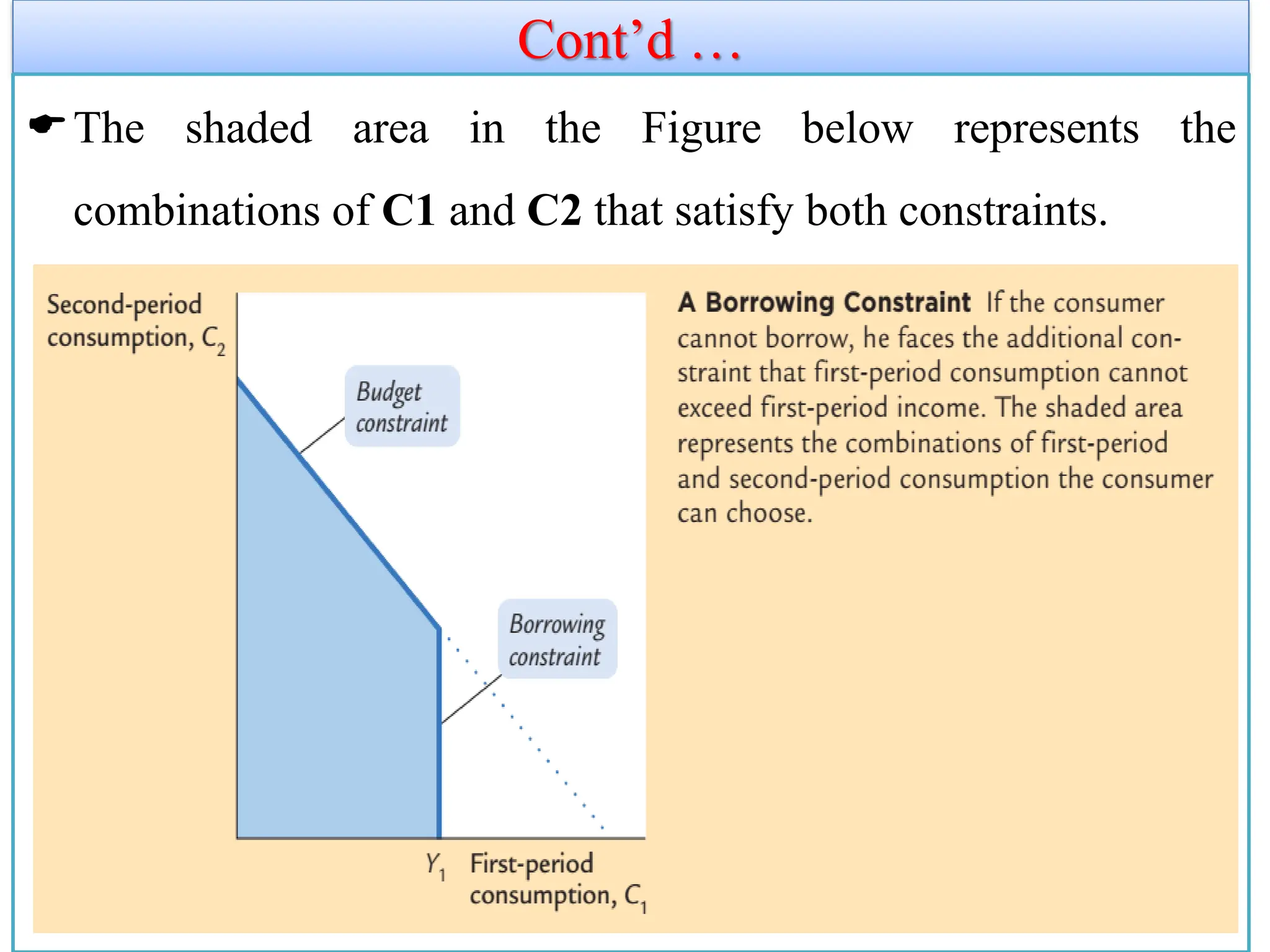
The shaded area in the Figure below represents the
combinations of C1 and C2 that satisfy both constraints.
11/26/2021 49

50. Cont’d …
✓ The borrowing constraint affects the consumption decision
✓ When the consumer faces a borrowing constraint, there are two
possible situations.
✓ In panel (a), the consumer chooses first-period consumption to be
less than first-period income, so the borrowing constraint is not
necessary/binding and does not affect consumption in either period.
✓ In panel (b), the borrowing constraint is binding. The consumer
would like to borrow and choose point 𝐃. But because borrowing is
not allowed, the best available choice is point 𝐄. When the
borrowing constraint is binding, first-period consumption equals
first-period income.
11/26/2021

51. Cont’d …
11/26/2021 51

52. Cont’d …
❖To sum up, the analysis of borrowing constraints leads us to
conclude that there are two consumption functions.
✓ For some consumers, the borrowing constraint is not binding,
and consumption in both periods depends on the present value
of lifetime income, 𝐘𝟏 + [ 𝐘𝟐/(𝟏 + 𝐫 )].
✓ For other consumers, the borrowing constraint binds, and the
consumption function is
✓ 𝐂 𝟏 = 𝐘𝟏 and 𝐂 𝟐= 𝐘𝟐. Hence, for those consumers who
would like to borrow but cannot, consumption depends only on
current income.
11/26/2021 52

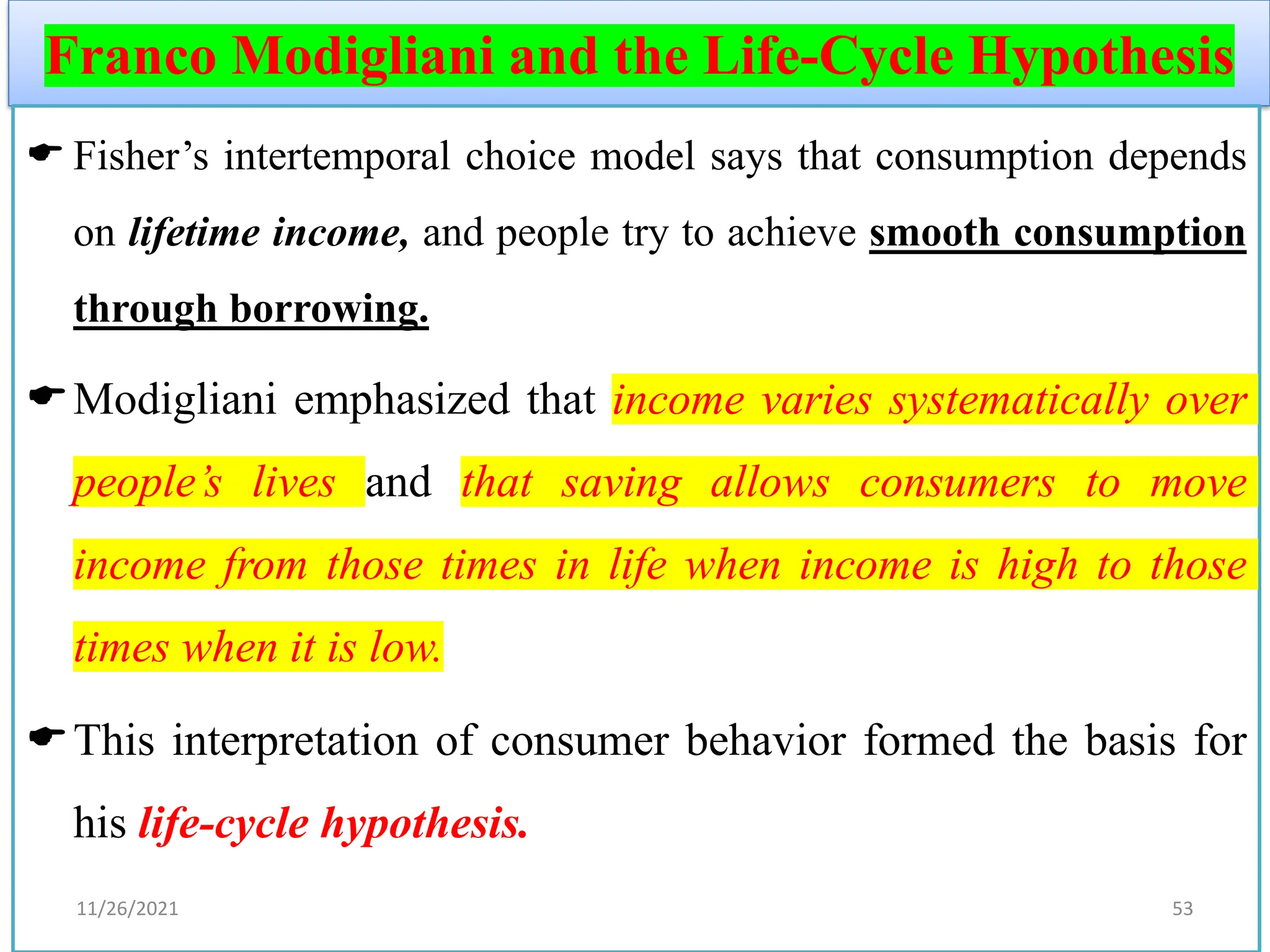
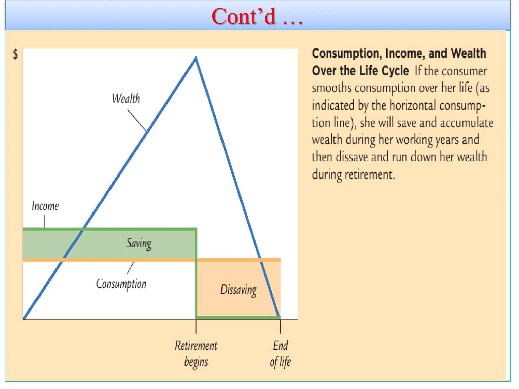
53. Franco Modigliani and the Life-Cycle Hypothesis
 Fisher’s intertemporal choice model says that consumption depends
on lifetime income, and people try to achieve smooth consumption
through borrowing.
Modigliani emphasized that income varies systematically over
people’s lives and that saving allows consumers to move
income from those times in life when income is high to those
times when it is low.
This interpretation of consumer behavior formed the basis for
his life-cycle hypothesis.
11/26/2021 53

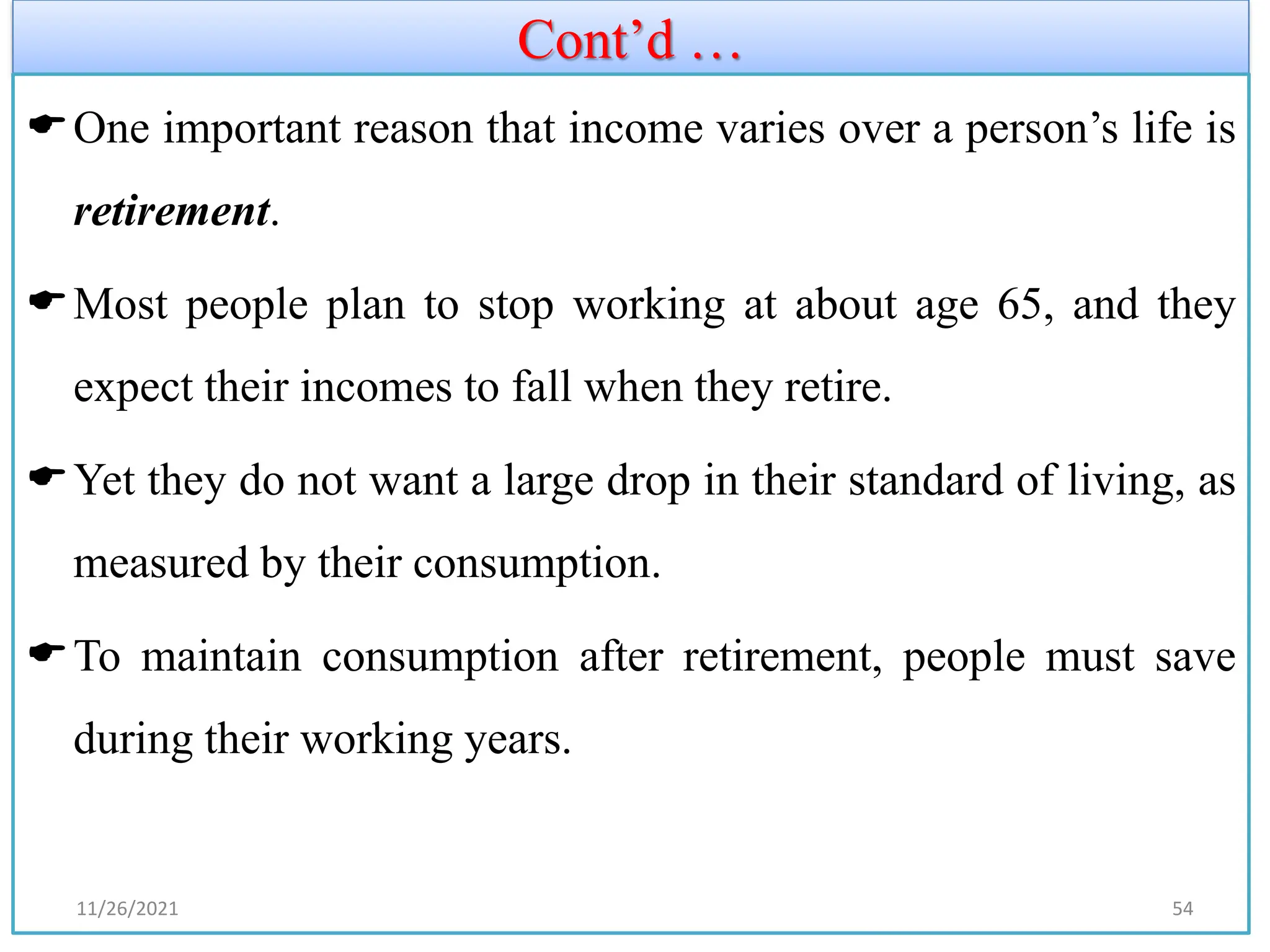
54. Cont’d …
One important reason that income varies over a person’s life is
retirement.
Most people plan to stop working at about age 65, and they
expect their incomes to fall when they retire.
Yet they do not want a large drop in their standard of living, as
measured by their consumption.
To maintain consumption after retirement, people must save
during their working years.
11/26/2021 54

55. Cont’d …
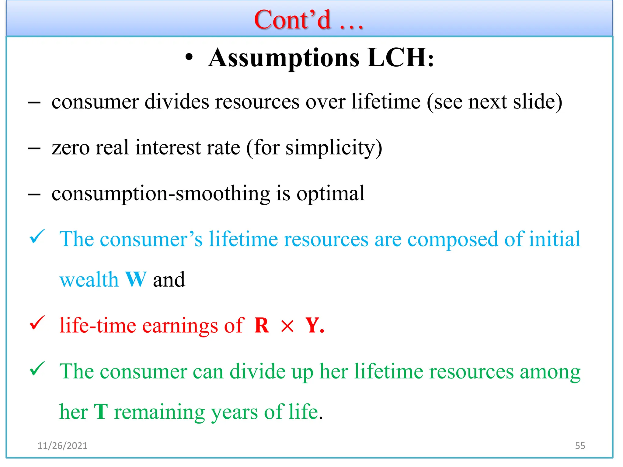
• Assumptions LCH:
– consumer divides resources over lifetime (see next slide)
– zero real interest rate (for simplicity)
– consumption-smoothing is optimal
✓ The consumer’s lifetime resources are composed of initial
wealth W and
✓ life-time earnings of 𝐑 × 𝐘.
✓ The consumer can divide up her lifetime resources among
her T remaining years of life.
11/26/2021 55

56. Cont’d …
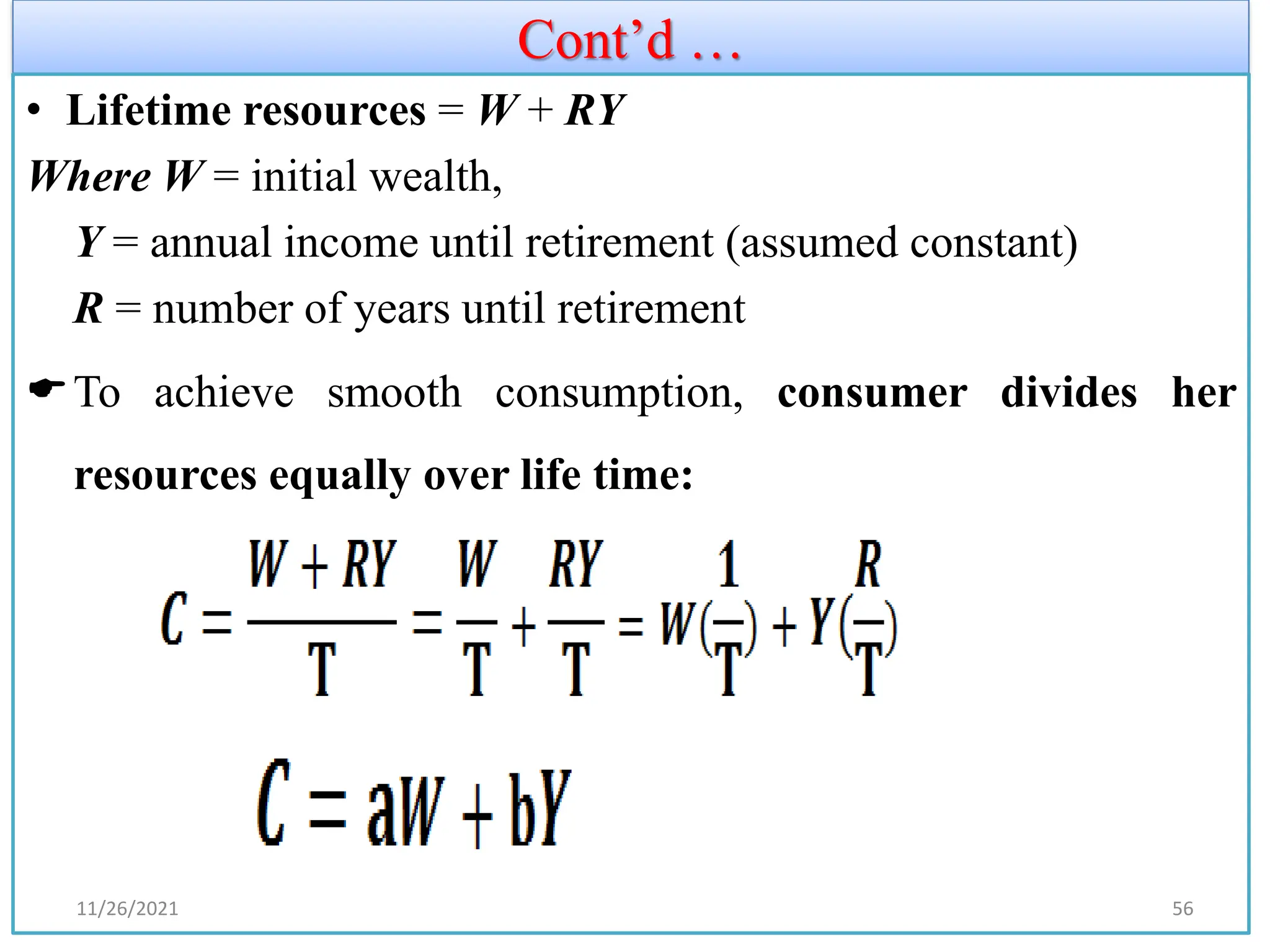
• Lifetime resources = W + RY
Where W = initial wealth,
Y = annual income until retirement (assumed constant)
R = number of years until retirement
To achieve smooth consumption, consumer divides her
resources equally over life time:
11/26/2021 56

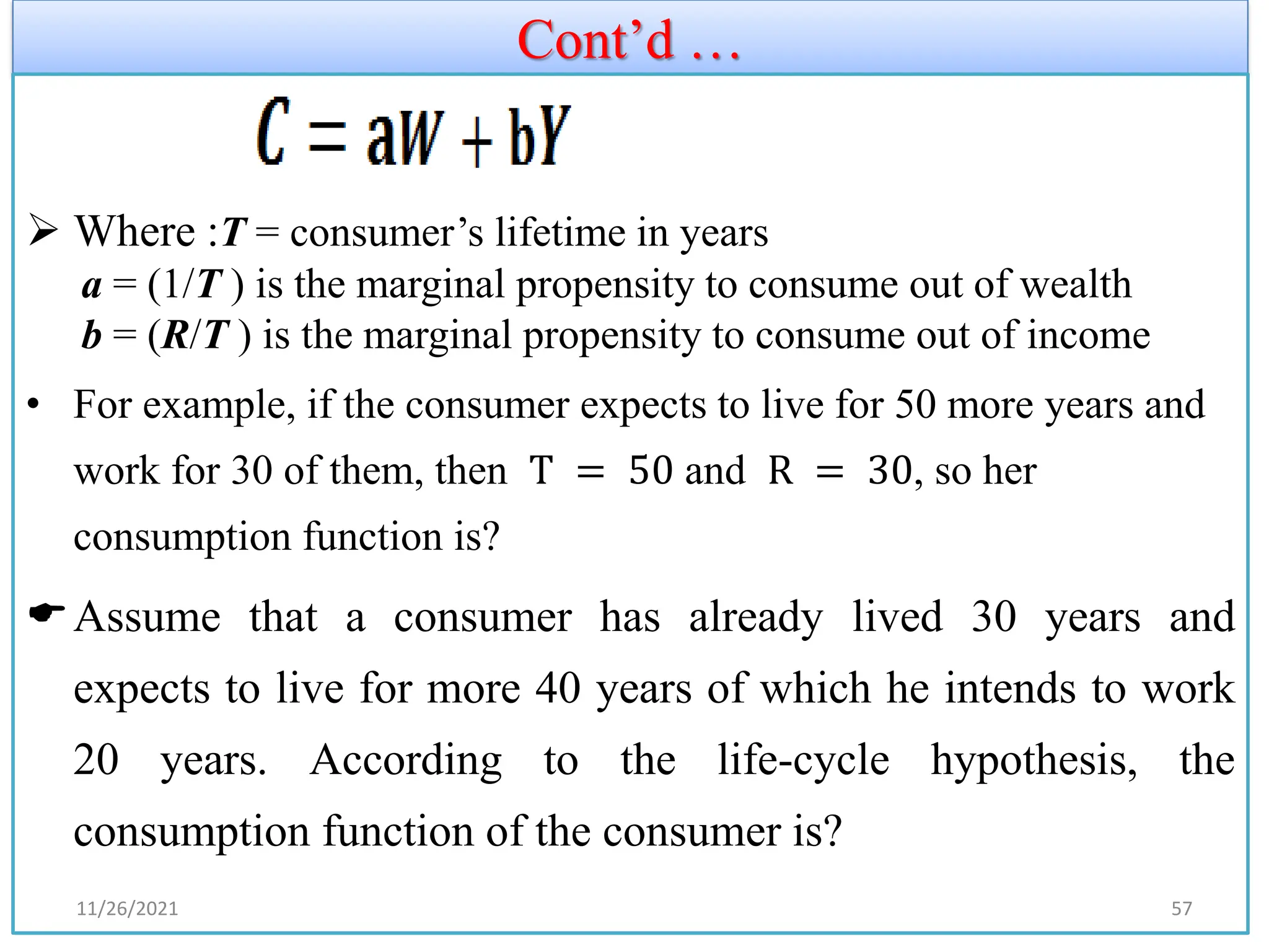
57. Cont’d …
➢ Where :T = consumer’s lifetime in years
a = (1/T ) is the marginal propensity to consume out of wealth
b = (R/T ) is the marginal propensity to consume out of income
• For example, if the consumer expects to live for 50 more years and
work for 30 of them, then T = 50 and R = 30, so her
consumption function is?
Assume that a consumer has already lived 30 years and
expects to live for more 40 years of which he intends to work
20 years. According to the life-cycle hypothesis, the
consumption function of the consumer is?
11/26/2021 57

58. Cont’d …
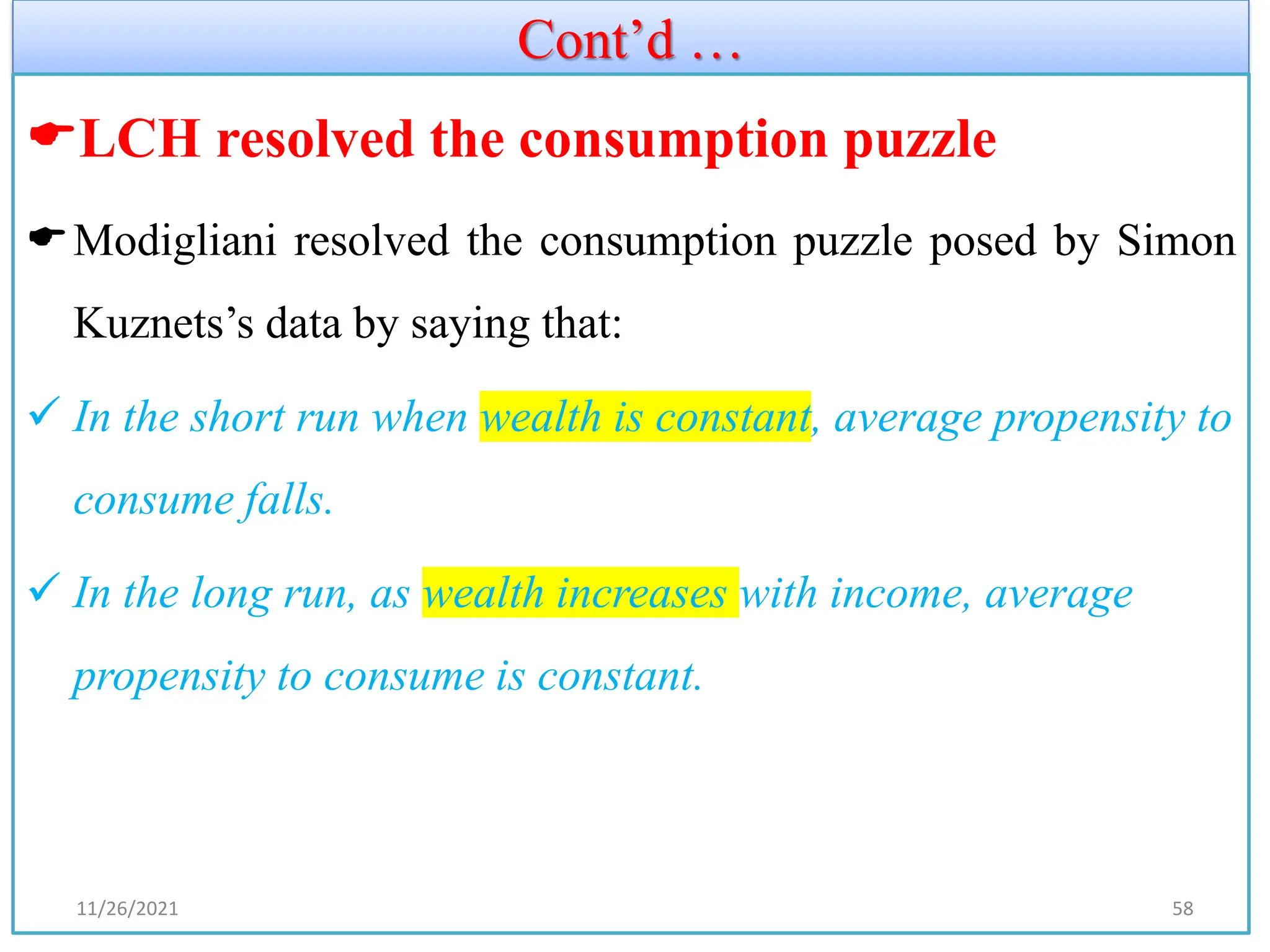
LCH resolved the consumption puzzle
Modigliani resolved the consumption puzzle posed by Simon
Kuznets’s data by saying that:
✓ In the short run when wealth is constant, average propensity to
consume falls.
✓ In the long run, as wealth increases with income, average
propensity to consume is constant.
11/26/2021 58

59. Cont’d …
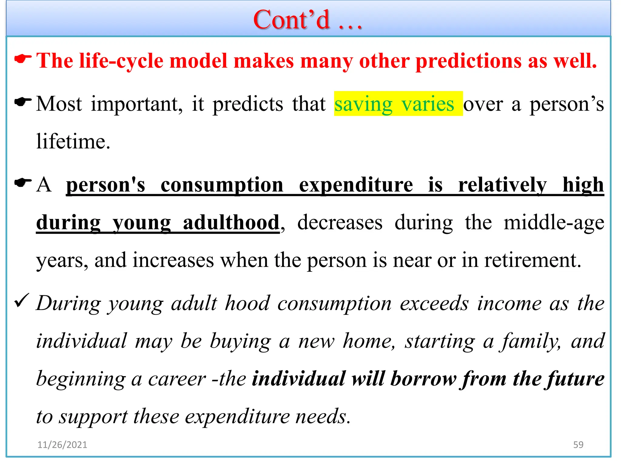
The life-cycle model makes many other predictions as well.
Most important, it predicts that saving varies over a person’s
lifetime.
A person's consumption expenditure is relatively high
during young adulthood, decreases during the middle-age
years, and increases when the person is near or in retirement.
✓ During young adult hood consumption exceeds income as the
individual may be buying a new home, starting a family, and
beginning a career -the individual will borrow from the future
to support these expenditure needs.
11/26/2021 59

60. Cont’d …
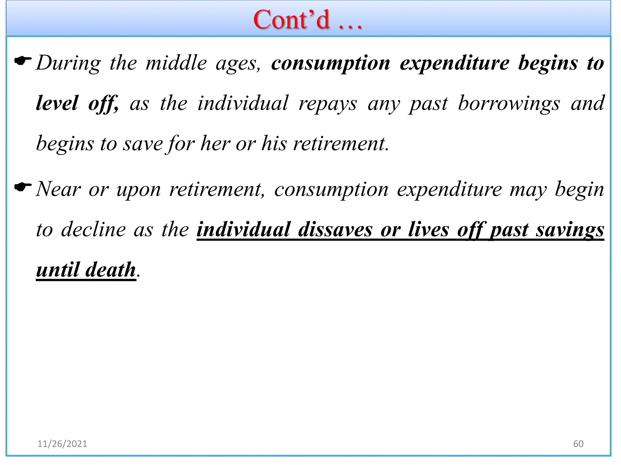
During the middle ages, consumption expenditure begins to
level off, as the individual repays any past borrowings and
begins to save for her or his retirement.
Near or upon retirement, consumption expenditure may begin
to decline as the individual dissaves or lives off past savings
until death.
11/26/2021 60

61. Cont’d …
11/26/2021 61

62. Milton Friedman and the Permanent-Income Hypothesis
Friedman’s permanent-income hypothesis complements
Modigliani’s life-cycle hypothesis:
 both use Irving Fisher’s theory of the consumer to argue that
consumption should not depend on current income alone.
But unlike the life-cycle hypothesis, which emphasizes that
income follows a regular pattern over a person’s lifetime.
 the permanent-income hypothesis emphasizes that people
experience random and temporary changes in their incomes
from year to year.
11/26/2021 62

63. Cont’d …
 Friedman suggested that we view current income Y as the sum of
two components, permanent income YP and transitory income YT .
That is,
Y = Y P + Y T
• Permanent income is the part of income that people expect to
persist into the future.
• Transitory income is the part of income that people do not expect to
persist.
• Friedman reasoned that consumption should depend primarily on
permanent income.
• Because consumers use saving and borrowing to smooth
consumption in response to transitory changes in income.
63

64. Cont’d …
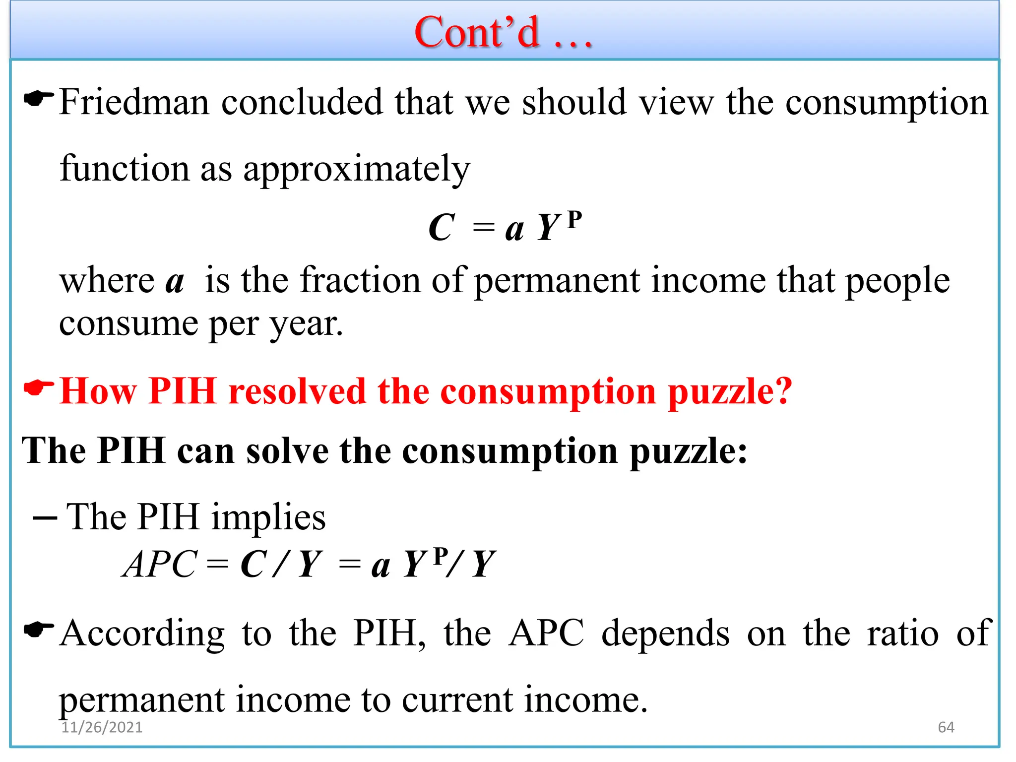
Friedman concluded that we should view the consumption
function as approximately
C = a Y P
where a is the fraction of permanent income that people
consume per year.
How PIH resolved the consumption puzzle?
The PIH can solve the consumption puzzle:
– The PIH implies
APC = C / Y = a Y P/ Y
According to the PIH, the APC depends on the ratio of
permanent income to current income.
11/26/2021 64

65. Cont’d …
✓ When current income temporarily rises above permanent
income, the APC temporarily falls;
✓ when current income temporarily falls below permanent
income, the APC temporarily rises.
✓Now consider the studies of household data.
❖Friedman reasoned that these data reflect a combination of
permanent and transitory income:
✓ Households with high permanent income have proportionately
higher consumption.
11/26/2021 65

66. Cont’d …
✓ If all variation in current income came from the permanent
component, the average propensity to consume would be the
same in all households.
✓ But some of the variation in income comes from the transitory
component, and households with high transitory income do not
have higher consumption.
Therefore, researchers find that high-income households have,
on average, lower average propensities to consume.
APC is lower in high-average income households.
11/26/2021 66

67. Cont’d …
✓ Similarly, consider the studies of time-series data.
✓ over long periods of time, the variation in income comes from
the permanent component.
✓ Hence, in long time-series, one should observe a constant
average propensity to consume, as in fact Kuznets found.
11/26/2021 67

68. 1.6).Robert Hall and the Random-Walk Hypothesis
❖The permanent-income hypothesis is based on Fisher’s model
of inter-temporal choice.
❖It builds on the idea that forward-looking consumers base their
consumption decisions not only on their current income but
also on the income they expect to receive in the future.
❖ Thus, the permanent-income hypothesis highlights that
consumption depends on people’s expectations.
❖Recent research on consumption has combined this view of the
consumer with the assumption of rational expectations.
68

69. 1.6).Robert Hall and the Random-Walk Hypothesis
❖The economist Robert Hall was the first to derive the
implications of rational expectations for consumption.
❖It is based on Fisher’s model & PIH, in which forward-looking
consumers base consumption on expected future income.
❖Hall adds the assumption of rational expectations, that people
use all available information to forecast future variables like
income.
❖The rational-expectations assumption states that people use all
available information to make optimal forecasts about the
future.
69

70. Cont’d …
He showed that if the permanent-income hypothesis is correct
and if consumers have rational expectations, then changes in
consumption over time should be unpredictable.
When changes in a variable are unpredictable, the variable is
said to follow a random walk.
According to Hall, the combination of the permanent-income
hypothesis and rational expectations implies that consumption
follows a random walk.
11/26/2021 70

71. Cont’d …
According to Hall, the combination of the PIH and
rational expectations implies that consumption follows a
random walk.
Hall reasoned as follows:
At any moment, consumers choose consumption based on
their current expectations of their lifetime incomes.
Over time, they change their consumption because they
receive news that causes them to revise their expectations.
11/26/2021 71

72. Cont’d …
In other words, changes in consumption reflect
“surprises” about lifetime income.
If consumers are optimally using all available information,
then they should be surprised only by events that were
entirely unpredictable.
Therefore, changes in their consumption should be
unpredictable as well.
11/26/2021 72

73. Cont’d …
✓ If RWH is correct and consumers have rational expectations,
then consumption should follow a random walk: changes in
consumption should be unpredictable.
– A change in income or wealth that was anticipated has
already been factored into expected permanent income, so
it will not change consumption.
– Only unanticipated changes in income or wealth that alter
expected permanent income will change consumption.
11/26/2021 73

74. Cont’d …
✓ The rational-expectations approach to consumption has
implications not only for forecasting but also for the analysis
of economic policies.
✓ If consumers obey the permanent-income hypothesis and
have rational expectations, then only unexpected policy
changes influence consumption.
✓ These policy changes take effect when they change
expectations.
11/26/2021 74

75. Cont’d …
For example, suppose that today the government passes a tax
increase to be effective next year.
In this case, consumers receive the news about their lifetime
incomes when the government passes the law (or even earlier
if the law’s passage was predictable).
The arrival of this news causes consumers to revise their
expectations and reduce their consumption.
11/26/2021 75

76. 1.7.The Psychology of Instant Gratification
• Theories from Fisher to Hall assume that
consumers are rational and act to maximize
lifetime utility.
• Recent studies by David Laibson and others
consider the psychology of consumers.
• The desire for instant gratification causes people
to save less than they rationally know they should

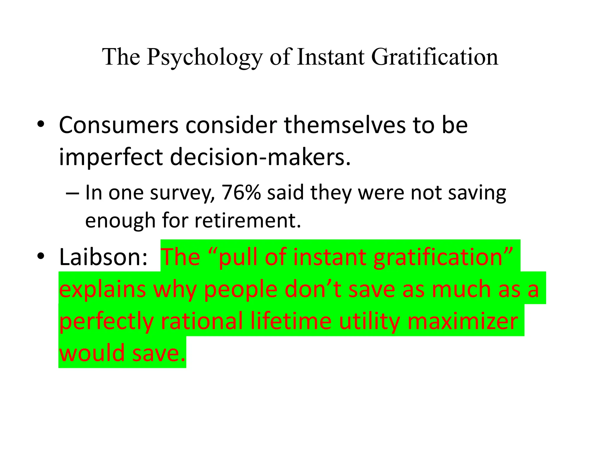
77. The Psychology of Instant Gratification
• Consumers consider themselves to be
imperfect decision-makers.
– In one survey, 76% said they were not saving
enough for retirement.
• Laibson: The “pull of instant gratification”
explains why people don’t save as much as a
perfectly rational lifetime utility maximizer
would save.

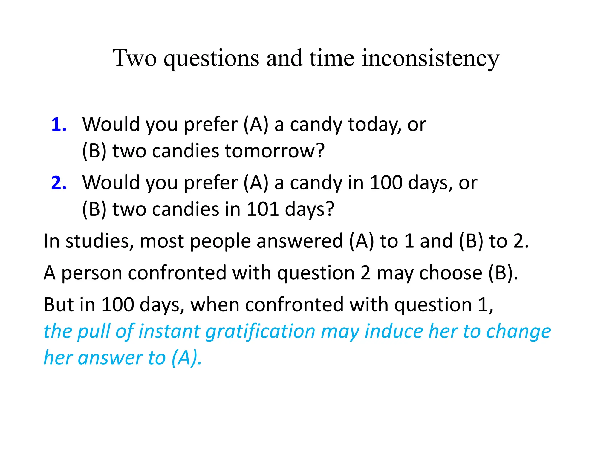
78. Two questions and time inconsistency
1. Would you prefer (A) a candy today, or
(B) two candies tomorrow?
2. Would you prefer (A) a candy in 100 days, or
(B) two candies in 101 days?
In studies, most people answered (A) to 1 and (B) to 2.
A person confronted with question 2 may choose (B).
But in 100 days, when confronted with question 1,
the pull of instant gratification may induce her to change
her answer to (A).

79. Cont’d …
Reading assignment on
adaptive and naïve expectation on
consumption
11/26/2021 79

80. Cont’d …
11/26/2021 80