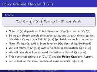
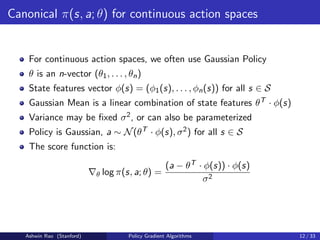
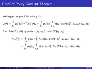
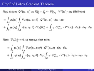
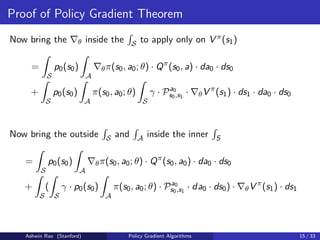
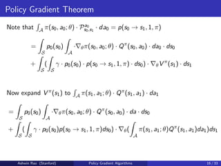
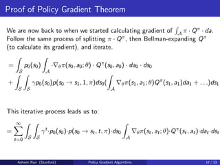
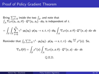
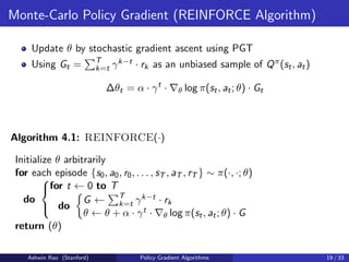
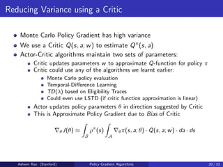
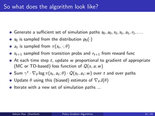
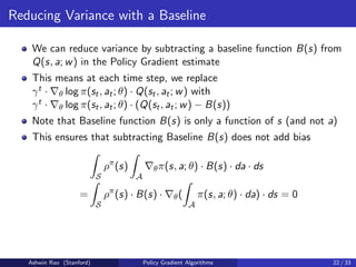
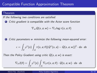
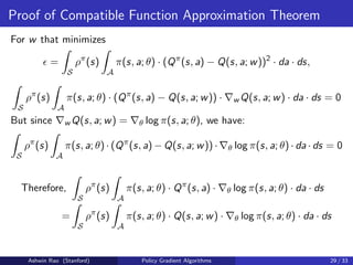
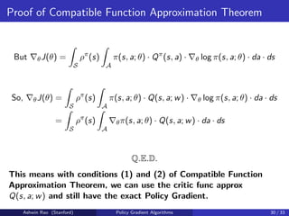
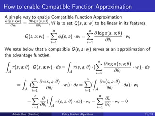
The document provides an overview of policy gradient algorithms. It begins by motivating policy gradients as a way to perform policy improvement with gradient ascent instead of argmax when the action space is large or continuous. It then defines key concepts like the policy gradient theorem, which shows the gradient of expected returns with respect to the policy parameters can be estimated by sampling simulation paths. It presents the policy gradient algorithm REINFORCE, which uses Monte Carlo returns to estimate the action-value function and perform policy gradient ascent updates. It also discusses canonical policy function approximations like the softmax policy for finite actions and Gaussian policy for continuous actions.

1. Policy Gradient Algorithms
Ashwin Rao
ICME, Stanford University
Ashwin Rao (Stanford) Policy Gradient Algorithms 1 / 33

2. Overview
1 Motivation and Intuition
2 Definitions and Notation
3 Policy Gradient Theorem and Proof
4 Policy Gradient Algorithms
5 Compatible Function Approximation Theorem and Proof
6 Natural Policy Gradient
Ashwin Rao (Stanford) Policy Gradient Algorithms 2 / 33

3. Why do we care about Policy Gradient (PG)?
Let us review how we got here
We started with Markov Decision Processes and Bellman Equations
Next we studied several variants of DP and RL algorithms
We noted that the idea of Generalized Policy Iteration (GPI) is key
Policy Improvement step: π(a|s) derived from argmaxa Q(s, a)
How do we do argmax when action space is large or continuous?
Idea: Do Policy Improvement step with a Gradient Ascent instead
Ashwin Rao (Stanford) Policy Gradient Algorithms 3 / 33

4. “Policy Improvement with a Gradient Ascent??”
We want to find the Policy that fetches the “Best Expected Returns”
Gradient Ascent on “Expected Returns” w.r.t params of Policy func
So we need a func approx for (stochastic) Policy Func: π(s, a; θ)
In addition to the usual func approx for Action Value Func: Q(s, a; w)
π(s, a; θ) func approx called Actor, Q(s, a; w) func approx called Critic
Critic parameters w are optimized w.r.t Q(s, a; w) loss function min
Actor parameters θ are optimized w.r.t Expected Returns max
We need to formally define “Expected Returns”
But we already see that this idea is appealing for continuous actions
GPI with Policy Improvement done as Policy Gradient (Ascent)
Ashwin Rao (Stanford) Policy Gradient Algorithms 4 / 33

5. Value Function-based and Policy-based RL
Value Function-based
Learn Value Function (with a function approximation)
Policy is implicit - readily derived from Value Function (eg: -greedy)
Policy-based
Learn Policy (with a function approximation)
No need to learn a Value Function
Actor-Critic
Learn Policy (Actor)
Learn Value Function (Critic)
Ashwin Rao (Stanford) Policy Gradient Algorithms 5 / 33

6. Advantages and Disadvantages of Policy Gradient approach
Advantages:
Finds the best Stochastic Policy (Optimal Deterministic Policy,
produced by other RL algorithms, can be unsuitable for POMDPs)
Naturally explores due to Stochastic Policy representation
Effective in high-dimensional or continuous action spaces
Small changes in θ ⇒ small changes in π, and in state distribution
This avoids the convergence issues seen in argmax-based algorithms
Disadvantages:
Typically converge to a local optimum rather than a global optimum
Policy Evaluation is typically inefficient and has high variance
Policy Improvement happens in small steps ⇒ slow convergence
Ashwin Rao (Stanford) Policy Gradient Algorithms 6 / 33

7. Notation
Discount Factor γ
Assume episodic with 0 ≤ γ ≤ 1 or non-episodic with 0 ≤ γ 1
States st ∈ S, Actions at ∈ A, Rewards rt ∈ R, ∀t ∈ {0, 1, 2, . . .}
State Transition Probabilities Pa
s,s0 = Pr(st+1 = s0|st = s, at = a)
Expected Rewards Ra
s = E[rt|st = s, at = a]
Initial State Probability Distribution p0 : S → [0, 1]
Policy Func Approx π(s, a; θ) = Pr(at = a|st = s, θ), θ ∈ Rk
PG coverage will be quite similar for non-discounted non-episodic, by
considering average-reward objective (so we won’t cover it)
Ashwin Rao (Stanford) Policy Gradient Algorithms 7 / 33

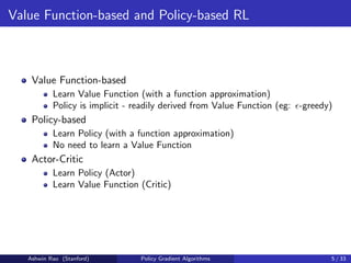
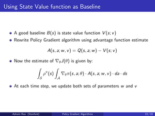
8. “Expected Returns” Objective
Now we formalize the “Expected Returns” Objective J(θ)
J(θ) = Eπ[
∞
X
t=0
γt
rt]
Value Function V π(s) and Action Value function Qπ(s, a) defined as:
V π
(s) = Eπ[
∞
X
k=t
γk−t
rk|st = s], ∀t ∈ {0, 1, 2, . . .}
Qπ
(s, a) = Eπ[
∞
X
k=t
γk−t
rk|st = s, at = a], ∀t ∈ {0, 1, 2, . . .}
Advantage Function Aπ
(s, a) = Qπ
(s, a) − V π
(s)
Also, p(s → s0, t, π) will be a key function for us - it denotes the
probability of going from state s to s0 in t steps by following policy π
Ashwin Rao (Stanford) Policy Gradient Algorithms 8 / 33

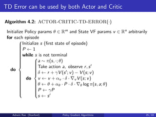
9. Discounted-Aggregate State-Visitation Measure
J(θ) = Eπ[
∞
X
t=0
γt
rt] =
∞
X
t=0
γt
Eπ[rt]
=
∞
X
t=0
γt
Z
S
(
Z
S
p0(s0) · p(s0 → s, t, π) · ds0)
Z
A
π(s, a; θ) · Ra
s · da · ds
=
Z
S
(
Z
S
∞
X
t=0
γt
· p0(s0) · p(s0 → s, t, π) · ds0)
Z
A
π(s, a; θ) · Ra
s · da · ds
Definition
J(θ) =
Z
S
ρπ
(s)
Z
A
π(s, a; θ) · Ra
s · da · ds
where ρπ(s) =
R
S
P∞
t=0 γt · p0(s0) · p(s0 → s, t, π) · ds0 is the key function
(for PG) we’ll refer to as Discounted-Aggregate State-Visitation Measure.
Ashwin Rao (Stanford) Policy Gradient Algorithms 9 / 33

10. Policy Gradient Theorem (PGT)
Theorem
∇θJ(θ) =
Z
S
ρπ
(s)
Z
A
∇θπ(s, a; θ) · Qπ
(s, a) · da · ds
Note: ρπ(s) depends on θ, but there’s no ∇θρπ(s) term in ∇θJ(θ)
So we can simply sample simulation paths, and at each time step, we
calculate (∇θ log π(s, a; θ)) · Qπ(s, a) (probabilities implicit in paths)
Note: ∇θ log π(s, a; θ) is Score function (Gradient of log-likelihood)
We will estimate Qπ(s, a) with a function approximation Q(s, a; w)
We will later show how to avoid the estimate bias of Q(s, a; w)
This numerical estimate of ∇θJ(θ) enables Policy Gradient Ascent
Let us look at the score function of some canonical π(s, a; θ)
Ashwin Rao (Stanford) Policy Gradient Algorithms 10 / 33

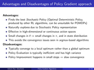
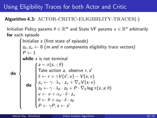
11. Canonical π(s, a; θ) for finite action spaces
For finite action spaces, we often use Softmax Policy
θ is an n-vector (θ1, . . . , θn)
Features vector φ(s, a) = (φ1(s, a), . . . , φn(s, a)) for all s ∈ S, a ∈ A
Weight actions using linear combinations of features: θT · φ(s, a)
Action probabilities proportional to exponentiated weights:
π(s, a; θ) =
eθT ·φ(s,a)
P
b eθT ·φ(s,b)
for all s ∈ S, a ∈ A
The score function is:
∇θ log π(s, a; θ) = φ(s, a)−
X
b
π(s, b; θ)·φ(s, b) = φ(s, a)−Eπ[φ(s, ·)]
Ashwin Rao (Stanford) Policy Gradient Algorithms 11 / 33

12. Canonical π(s, a; θ) for continuous action spaces
For continuous action spaces, we often use Gaussian Policy
θ is an n-vector (θ1, . . . , θn)
State features vector φ(s) = (φ1(s), . . . , φn(s)) for all s ∈ S
Gaussian Mean is a linear combination of state features θT · φ(s)
Variance may be fixed σ2, or can also be parameterized
Policy is Gaussian, a ∼ N(θT · φ(s), σ2) for all s ∈ S
The score function is:
∇θ log π(s, a; θ) =
(a − θT · φ(s)) · φ(s)
σ2
Ashwin Rao (Stanford) Policy Gradient Algorithms 12 / 33

13. Proof of Policy Gradient Theorem
We begin the proof by noting that:
J(θ) =
Z
S
p0(s0)·V π
(s0)·ds0 =
Z
S
p0(s0)
Z
A
π(s0, a0; θ)·Qπ
(s0, a0)·da0·ds0
Calculate ∇θJ(θ) by parts π(s0, a0; θ) and Qπ(s0, a0)
∇θJ(θ) =
Z
S
p0(s0)
Z
A
∇θπ(s0, a0; θ) · Qπ
(s0, a0) · da0 · ds0
+
Z
S
p0(s0)
Z
A
π(s0, a0; θ) · ∇θQπ
(s0, a0) · da0 · ds0
Ashwin Rao (Stanford) Policy Gradient Algorithms 13 / 33

14. Proof of Policy Gradient Theorem
Now expand Qπ(s0, a0) as Ra0
s0
+
R
S γ · Pa0
s0,s1
· V π(s1) · ds1 (Bellman)
=
Z
S
p0(s0)
Z
A
∇θπ(s0, a0; θ) · Qπ
(s0, a0) · da0 · ds0
+
Z
S
p0(s0)
Z
A
π(s0, a0; θ) · ∇θ(Ra0
s0
+
Z
S
γ · Pa0
s0,s1
· V π
(s1) · ds1) · da0 · ds0
Note: ∇θRa0
s0
= 0, so remove that term
=
Z
S
p0(s0)
Z
A
∇θπ(s0, a0; θ) · Qπ
(s0, a) · da0 · ds0
+
Z
S
p0(s0)
Z
A
π(s0, a0; θ) · ∇θ(
Z
S
γ · Pa0
s0,s1
· V π
(s1) · ds1) · da0 · ds0
Ashwin Rao (Stanford) Policy Gradient Algorithms 14 / 33

15. Proof of Policy Gradient Theorem
Now bring the ∇θ inside the
R
S to apply only on V π(s1)
=
Z
S
p0(s0)
Z
A
∇θπ(s0, a0; θ) · Qπ
(s0, a) · da0 · ds0
+
Z
S
p0(s0)
Z
A
π(s0, a0; θ)
Z
S
γ · Pa0
s0,s1
· ∇θV π
(s1) · ds1 · da0 · ds0
Now bring the outside
R
S and
R
A inside the inner
R
S
=
Z
S
p0(s0)
Z
A
∇θπ(s0, a0; θ) · Qπ
(s0, a0) · da0 · ds0
+
Z
S
(
Z
S
γ · p0(s0)
Z
A
π(s0, a0; θ) · Pa0
s0,s1
· da0 · ds0) · ∇θV π
(s1) · ds1
Ashwin Rao (Stanford) Policy Gradient Algorithms 15 / 33

16. Policy Gradient Theorem
Note that
R
A π(s0, a0; θ) · Pa0
s0,s1
· da0 = p(s0 → s1, 1, π)
=
Z
S
p0(s0)
Z
A
·∇θπ(s0, a0; θ) · Qπ
(s0, a0) · da0 · ds0
+
Z
S
(
Z
S
γ · p0(s0) · p(s0 → s1, 1, π) · ds0) · ∇θV π
(s1) · ds1
Now expand V π(s1) to
R
A π(s1, a1; θ) · Qπ(s1, a1) · da1
=
Z
S
p0(s0)
Z
A
·∇θπ(s0, a0; θ) · Qπ
(s0, a0) · da · ds0
+
Z
S
(
Z
S
γ · p0(s0)p(s0 → s1, 1, π)ds0) · ∇θ(
Z
A
π(s1, a1; θ)Qπ
(s1, a1)da1)ds1
Ashwin Rao (Stanford) Policy Gradient Algorithms 16 / 33

17. Proof of Policy Gradient Theorem
We are now back to when we started calculating gradient of
R
A π · Qπ · da.
Follow the same process of splitting π · Qπ, then Bellman-expanding Qπ
(to calculate its gradient), and iterate.
=
Z
S
p0(s0)
Z
A
·∇θπ(s0, a0; θ) · Qπ
(s0, a0) · da0 · ds0
+
Z
S
Z
S
γp0(s0)p(s0 → s1, 1, π)ds0(
Z
A
∇θπ(s1, a1; θ)Qπ
(s1, a1)da1 + . . .)ds1
This iterative process leads us to:
=
∞
X
t=0
Z
S
Z
S
γt
·p0(s0)·p(s0 → st, t, π)·ds0
Z
A
∇θπ(st, at; θ)·Qπ
(st, at)·dat·dst
Ashwin Rao (Stanford) Policy Gradient Algorithms 17 / 33

18. Proof of Policy Gradient Theorem
Bring
P∞
t=0 inside the two
R
S, and note that
R
A ∇θπ(st, at; θ) · Qπ(st, at) · dat is independent of t.
=
Z
S
Z
S
∞
X
t=0
γt
·p0(s0)·p(s0 → s, t, π)·ds0
Z
A
∇θπ(s, a; θ)·Qπ
(s, a)·da·ds
Reminder that
R
S
P∞
t=0 γt · p0(s0) · p(s0 → s, t, π) · ds0
def
= ρπ(s). So,
∇θJ(θ) =
Z
S
ρπ
(s)
Z
A
∇θπ(s, a; θ) · Qπ
(s, a) · da · ds
Q.E.D.
Ashwin Rao (Stanford) Policy Gradient Algorithms 18 / 33

19. Monte-Carlo Policy Gradient (REINFORCE Algorithm)
Update θ by stochastic gradient ascent using PGT
Using Gt =
PT
k=t γk−t · rk as an unbiased sample of Qπ(st, at)
∆θt = α · γt
· ∇θ log π(st, at; θ) · Gt
Algorithm 4.1: REINFORCE(·)
Initialize θ arbitrarily
for each episode {s0, a0, r0, . . . , sT , aT , rT } ∼ π(·, ·; θ)
do



for t ← 0 to T
do
G ←
PT
k=t γk−t · rk
θ ← θ + α · γt · ∇θ log π(st, at; θ) · G
return (θ)
Ashwin Rao (Stanford) Policy Gradient Algorithms 19 / 33

20. Reducing Variance using a Critic
Monte Carlo Policy Gradient has high variance
We use a Critic Q(s, a; w) to estimate Qπ(s, a)
Actor-Critic algorithms maintain two sets of parameters:
Critic updates parameters w to approximate Q-function for policy π
Critic could use any of the algorithms we learnt earlier:
Monte Carlo policy evaluation
Temporal-Difference Learning
TD(λ) based on Eligibility Traces
Could even use LSTD (if critic function approximation is linear)
Actor updates policy parameters θ in direction suggested by Critic
This is Approximate Policy Gradient due to Bias of Critic
∇θJ(θ) ≈
Z
S
ρπ
(s)
Z
A
∇θπ(s, a; θ) · Q(s, a; w) · da · ds
Ashwin Rao (Stanford) Policy Gradient Algorithms 20 / 33

21. So what does the algorithm look like?
Generate a sufficient set of simulation paths s0, a0, r0, s1, a1, r1, . . .
s0 is sampled from the distribution p0(·)
at is sampled from π(st, ·; θ)
st+1 sampled from transition probs and rt+1 from reward func
At each time step t, update w proportional to gradient of appropriate
(MC or TD-based) loss function of Q(s, a; w)
Sum γt · ∇θ log π(st, at; θ) · Q(st, at; w) over t and over paths
Update θ using this (biased) estimate of ∇θJ(θ)
Iterate with a new set of simulation paths ...
Ashwin Rao (Stanford) Policy Gradient Algorithms 21 / 33

22. Reducing Variance with a Baseline
We can reduce variance by subtracting a baseline function B(s) from
Q(s, a; w) in the Policy Gradient estimate
This means at each time step, we replace
γt · ∇θ log π(st, at; θ) · Q(st, at; w) with
γt · ∇θ log π(st, at; θ) · (Q(st, at; w) − B(s))
Note that Baseline function B(s) is only a function of s (and not a)
This ensures that subtracting Baseline B(s) does not add bias
Z
S
ρπ
(s)
Z
A
∇θπ(s, a; θ) · B(s) · da · ds
=
Z
S
ρπ
(s) · B(s) · ∇θ(
Z
A
π(s, a; θ) · da) · ds = 0
Ashwin Rao (Stanford) Policy Gradient Algorithms 22 / 33

23. Using State Value function as Baseline
A good baseline B(s) is state value function V (s; v)
Rewrite Policy Gradient algorithm using advantage function estimate
A(s, a; w, v) = Q(s, a; w) − V (s; v)
Now the estimate of ∇θJ(θ) is given by:
Z
S
ρπ
(s)
Z
A
∇θπ(s, a; θ) · A(s, a; w, v) · da · ds
At each time step, we update both sets of parameters w and v
Ashwin Rao (Stanford) Policy Gradient Algorithms 23 / 33

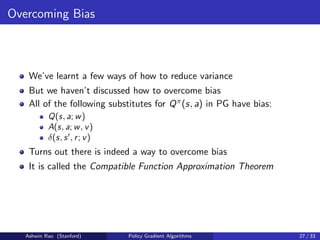
24. TD Error as estimate of Advantage Function
Consider TD error δπ for the true Value Function V π(s)
δπ
= r + γV π
(s0
) − V π
(s)
δπ is an unbiased estimate of Advantage function Aπ(s, a)
Eπ[δπ
|s, a] = Eπ[r+γV π
(s0
)|s, a]−V π
(s) = Qπ
(s, a)−V π
(s) = Aπ
(s, a)
So we can write Policy Gradient in terms of Eπ[δπ|s, a]
∇θJ(θ) =
Z
S
ρπ
(s)
Z
A
∇θπ(s, a; θ) · Eπ[δπ
|s, a] · da · ds
In practice, we can use func approx for TD error (and sample):
δ(s, r, s0
; v) = r + γV (s0
; v) − V (s; v)
This approach requires only one set of critic parameters v
Ashwin Rao (Stanford) Policy Gradient Algorithms 24 / 33

25. TD Error can be used by both Actor and Critic
Algorithm 4.2: ACTOR-CRITIC-TD-ERROR(·)
Initialize Policy params θ ∈ Rm and State VF params v ∈ Rn arbitrarily
for each episode
do































Initialize s (first state of episode)
P ← 1
while s is not terminal
do



















a ∼ π(s, ·; θ)
Take action a, observe r, s0
δ ← r + γV (s0; v) − V (s; v)
v ← v + αv · δ · ∇v V (s; v)
θ ← θ + αθ · P · δ · ∇θ log π(s, a; θ)
P ← γP
s ← s0
Ashwin Rao (Stanford) Policy Gradient Algorithms 25 / 33

26. Using Eligibility Traces for both Actor and Critic
Algorithm 4.3: ACTOR-CRITIC-ELIGIBILITY-TRACES(·)
Initialize Policy params θ ∈ Rm and State VF params v ∈ Rn arbitrarily
for each episode
do









































Initialize s (first state of episode)
zθ, zv ← 0 (m and n components eligibility trace vectors)
P ← 1
while s is not terminal
do























a ∼ π(s, ·; θ)
Take action a, observe r, s0
δ ← r + γV (s0; v) − V (s; v)
zv ← γ · λv · zv + ∇v V (s; v)
zθ ← γ · λθ · zθ + P · ∇θ log π(s, a; θ)
v ← v + αv · δ · zv
θ ← θ + αθ · δ · zθ
P ← γP, s ← s0
Ashwin Rao (Stanford) Policy Gradient Algorithms 26 / 33

27. Overcoming Bias
We’ve learnt a few ways of how to reduce variance
But we haven’t discussed how to overcome bias
All of the following substitutes for Qπ(s, a) in PG have bias:
Q(s, a; w)
A(s, a; w, v)
δ(s, s0
, r; v)
Turns out there is indeed a way to overcome bias
It is called the Compatible Function Approximation Theorem
Ashwin Rao (Stanford) Policy Gradient Algorithms 27 / 33

28. Compatible Function Approximation Theorem
Theorem
If the following two conditions are satisfied:
1 Critic gradient is compatible with the Actor score function
∇w Q(s, a; w) = ∇θ log π(s, a; θ)
2 Critic parameters w minimize the following mean-squared error:
=
Z
S
ρπ
(s)
Z
A
π(s, a; θ)(Qπ
(s, a) − Q(s, a; w))2
· da · ds
Then the Policy Gradient using critic Q(s, a; w) is exact:
∇θJ(θ) =
Z
S
ρπ
(s)
Z
A
∇θπ(s, a; θ) · Q(s, a; w) · da · ds
Ashwin Rao (Stanford) Policy Gradient Algorithms 28 / 33

29. Proof of Compatible Function Approximation Theorem
For w that minimizes
=
Z
S
ρπ
(s)
Z
A
π(s, a; θ) · (Qπ
(s, a) − Q(s, a; w))2
· da · ds,
Z
S
ρπ
(s)
Z
A
π(s, a; θ) · (Qπ
(s, a) − Q(s, a; w)) · ∇w Q(s, a; w) · da · ds = 0
But since ∇w Q(s, a; w) = ∇θ log π(s, a; θ), we have:
Z
S
ρπ
(s)
Z
A
π(s, a; θ) · (Qπ
(s, a) − Q(s, a; w)) · ∇θ log π(s, a; θ) · da · ds = 0
Therefore,
Z
S
ρπ
(s)
Z
A
π(s, a; θ) · Qπ
(s, a) · ∇θ log π(s, a; θ) · da · ds
=
Z
S
ρπ
(s)
Z
A
π(s, a; θ) · Q(s, a; w) · ∇θ log π(s, a; θ) · da · ds
Ashwin Rao (Stanford) Policy Gradient Algorithms 29 / 33

30. Proof of Compatible Function Approximation Theorem
But ∇θJ(θ) =
Z
S
ρπ
(s)
Z
A
π(s, a; θ) · Qπ
(s, a) · ∇θ log π(s, a; θ) · da · ds
So, ∇θJ(θ) =
Z
S
ρπ
(s)
Z
A
π(s, a; θ) · Q(s, a; w) · ∇θ log π(s, a; θ) · da · ds
=
Z
S
ρπ
(s)
Z
A
∇θπ(s, a; θ) · Q(s, a; w) · da · ds
Q.E.D.
This means with conditions (1) and (2) of Compatible Function
Approximation Theorem, we can use the critic func approx
Q(s, a; w) and still have the exact Policy Gradient.
Ashwin Rao (Stanford) Policy Gradient Algorithms 30 / 33

31. How to enable Compatible Function Approximation
A simple way to enable Compatible Function Approximation
∂Q(s,a;w)
∂wi
= ∂ log π(s,a;θ)
∂θi
, ∀i is to set Q(s, a; w) to be linear in its features.
Q(s, a; w) =
n
X
i=1
φi (s, a) · wi =
n
X
i=1
∂ log π(s, a; θ)
∂θi
· wi
We note below that a compatible Q(s, a; w) serves as an approximation of
the advantage function.
Z
A
π(s, a; θ) · Q(s, a; w) · da =
Z
A
π(s, a; θ) · (
n
X
i=1
∂ log π(s, a; θ)
∂θi
· wi ) · da
=
Z
A
·(
n
X
i=1
∂π(s, a; θ)
∂θi
· wi ) · da =
n
X
i=1
(
Z
A
∂π(s, a; θ)
∂θi
· da) · wi
=
n
X
i=1
∂
∂θi
(
Z
A
π(s, a; θ) · da) · wi =
n
X
i=1
∂1
∂θi
· wi = 0
Ashwin Rao (Stanford) Policy Gradient Algorithms 31 / 33

32. Fisher Information Matrix
Denoting [∂ log π(s,a;θ)
∂θi
], i = 1, . . . , n as the score column vector SC(s, a; θ)
and assuming compatible linear-approx critic:
∇θJ(θ) =
Z
S
ρπ
(s)
Z
A
π(s, a; θ) · (SC(s, a; θ) · SC(s, a; θ)T
· w) · da · ds
= Es∼ρπ,a∼π[SC(s, a; θ) · SC(s, a; θ)T
] · w
= FIMρπ,π(θ) · w
where FIMρπ,π(θ) is the Fisher Information Matrix w.r.t. s ∼ ρπ, a ∼ π.
Ashwin Rao (Stanford) Policy Gradient Algorithms 32 / 33

33. Natural Policy Gradient
Recall the idea of Natural Gradient from Numerical Optimization
Natural gradient ∇nat
θ J(θ) is the direction of optimal θ movement
In terms of the KL-divergence metric (versus plain Euclidean norm)
Natural gradient yields better convergence (we won’t cover proof)
Formally defined as: ∇θJ(θ) = FIMρπ,π(θ) · ∇nat
θ J(θ)
Therefore, ∇nat
θ J(θ) = w
This compact result is great for our algorithm:
Update Critic params w with the critic loss gradient (at step t) as:
γt
· (rt + γ · SC(st+1, at+1, θ) · w − SC(st, at, θ) · w) · SC(st, at, θ)
Update Actor params θ in the direction equal to value of w
Ashwin Rao (Stanford) Policy Gradient Algorithms 33 / 33