Downloaded 38 times
![Anchors - Example
• Anchor dims=(size*scale)/sqrt(ratio)
• Eg for 32 anchor size:
• [-22 -11 22 11] 44X22 [-28 -14 28 14] 56X28 [-35 -17 35 17] 70X34
• [-16 -16 16 16] 32X32 [-20 -20 20 20] 40X40 [-25 -25 25 25] 50X50
• [-11 -22 11 22] 22X44 [-14 -28 14 28] 28X56 [-17 -35 17 35] 34X70
For 800,600 input image:
• P3 activation map shape: 100,75
• Stride: 8
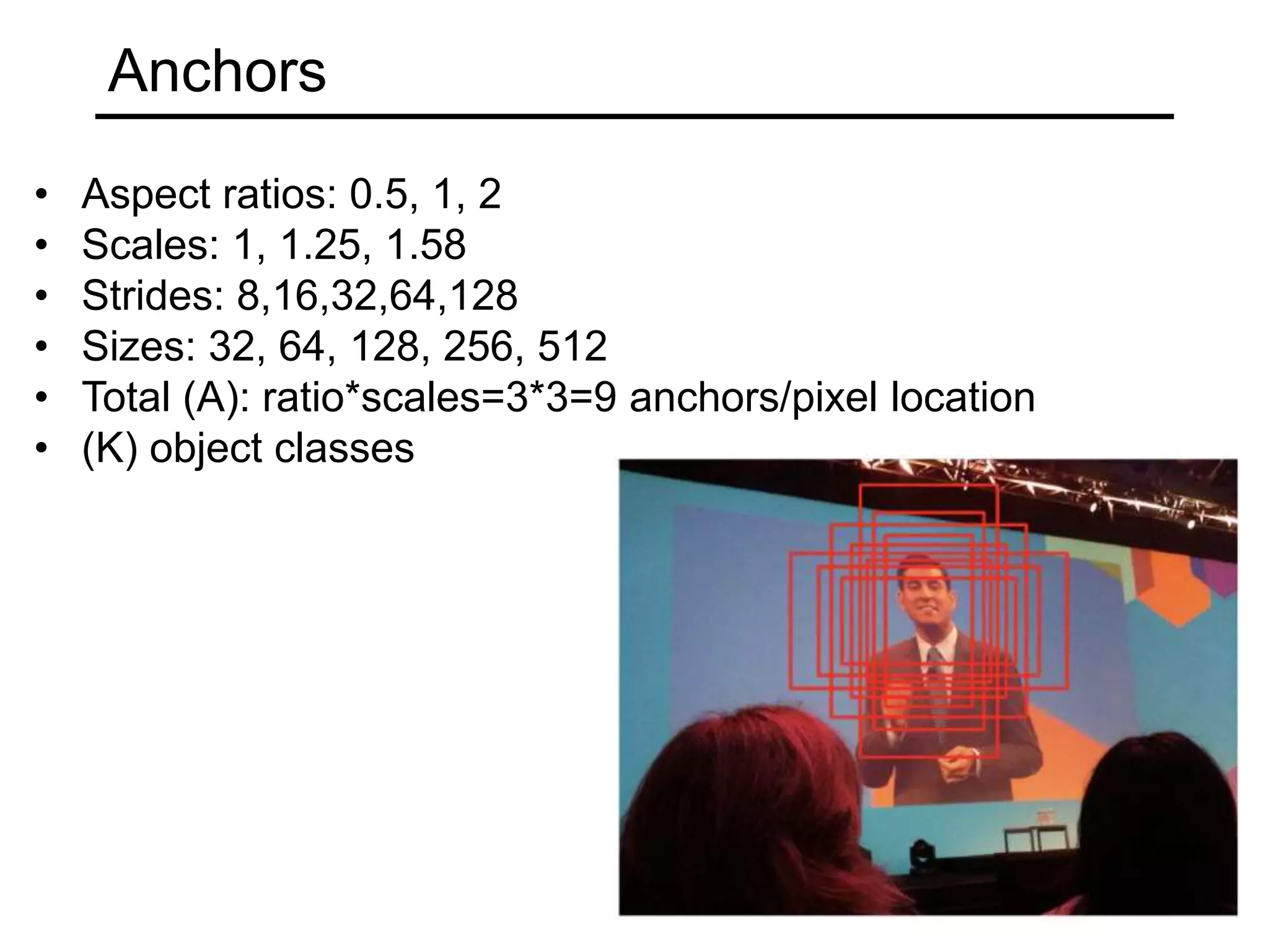
• Total (A) = 9 anchors per pixel location
• Total anchors at P3 level = 100*75*9
= 67500
• Similarly sum for all pyramid levels
P3,P4,P5,P6,P7 = total 90360! anchors per
image](https://image.slidesharecdn.com/objectdetection-190825033952/75/Object-detection-RCNNs-vs-Retinanet-36-2048.jpg)
![Shift anchors
Shift anchors according to input image from activation map
(26,15)
(-22,-11)
(22,11)
(-18,-7)
(0,0)
(4,4)
Shift anchor centered at (0,0) on P3 (stride 8)
Activation map by [ 4. 4. 4. 4.]
Next shift [ 12. 4. 12. 4.], [ 20. 4. 20. 4.] , ….
(4,4) (12,4)
8
Input Image
Anchors applied wrt to input image!](https://image.slidesharecdn.com/objectdetection-190825033952/75/Object-detection-RCNNs-vs-Retinanet-37-2048.jpg)


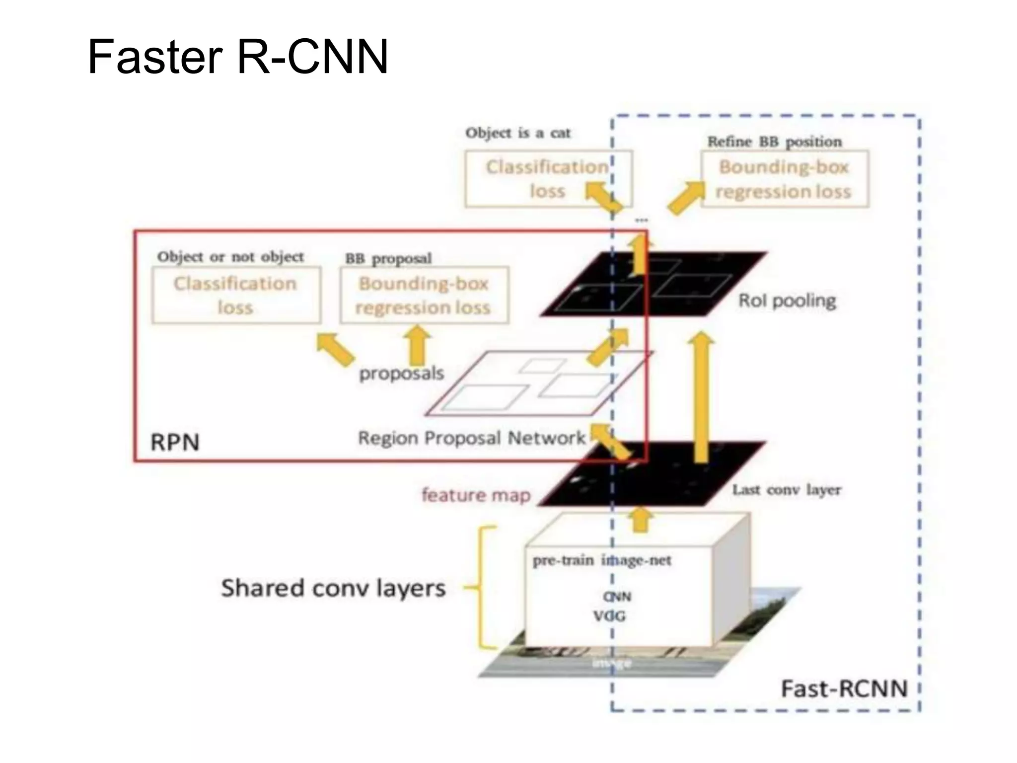
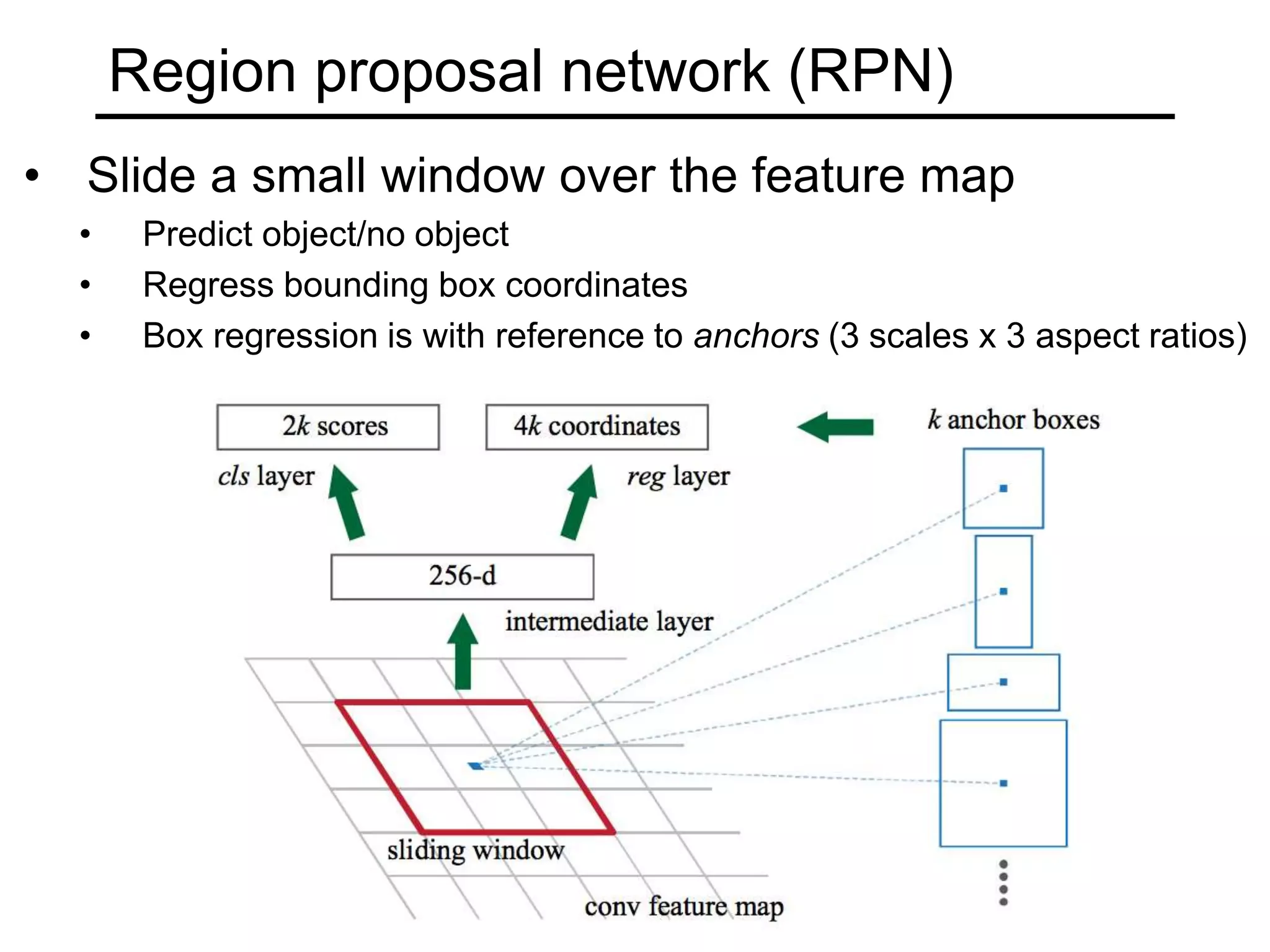
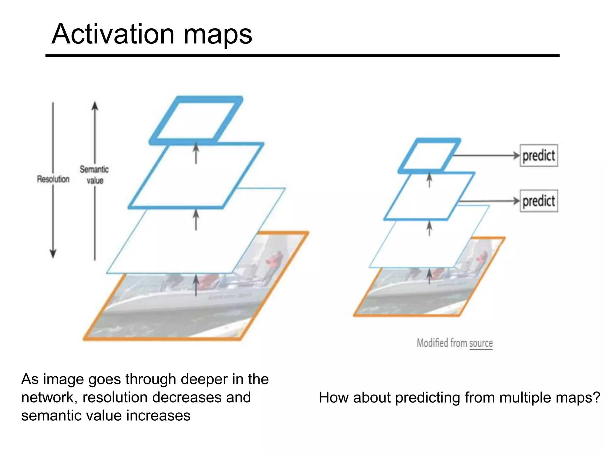
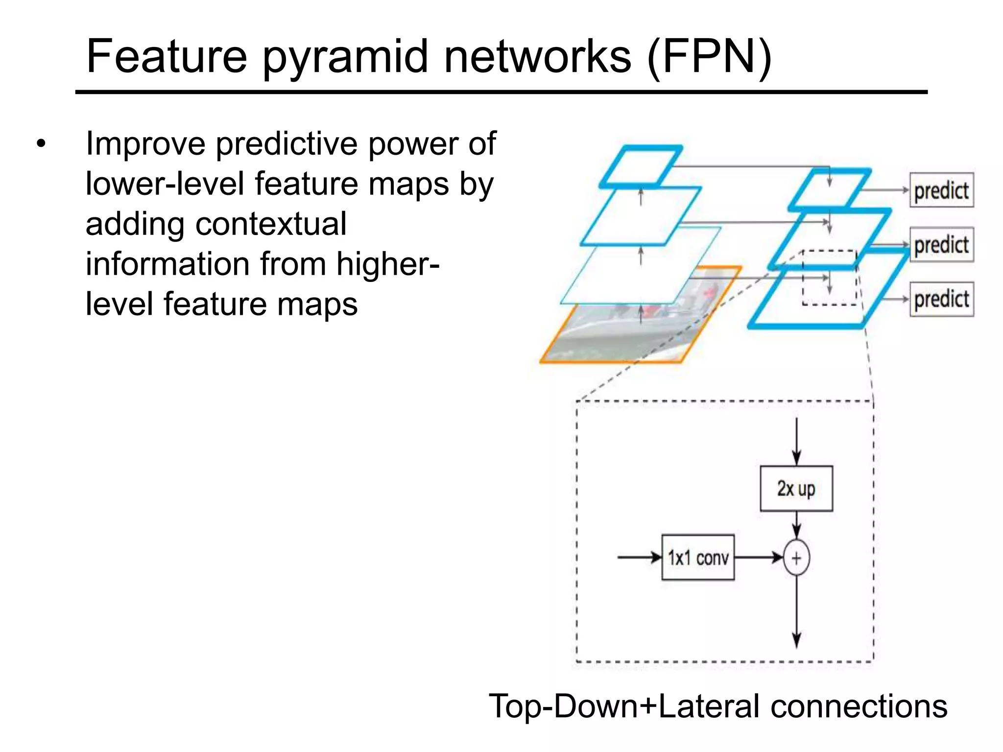
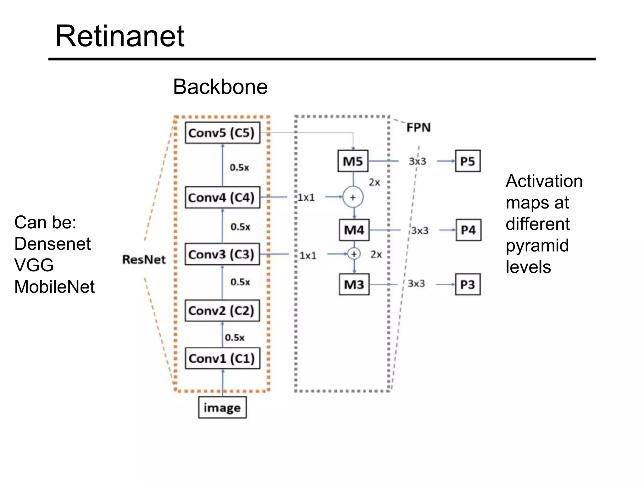
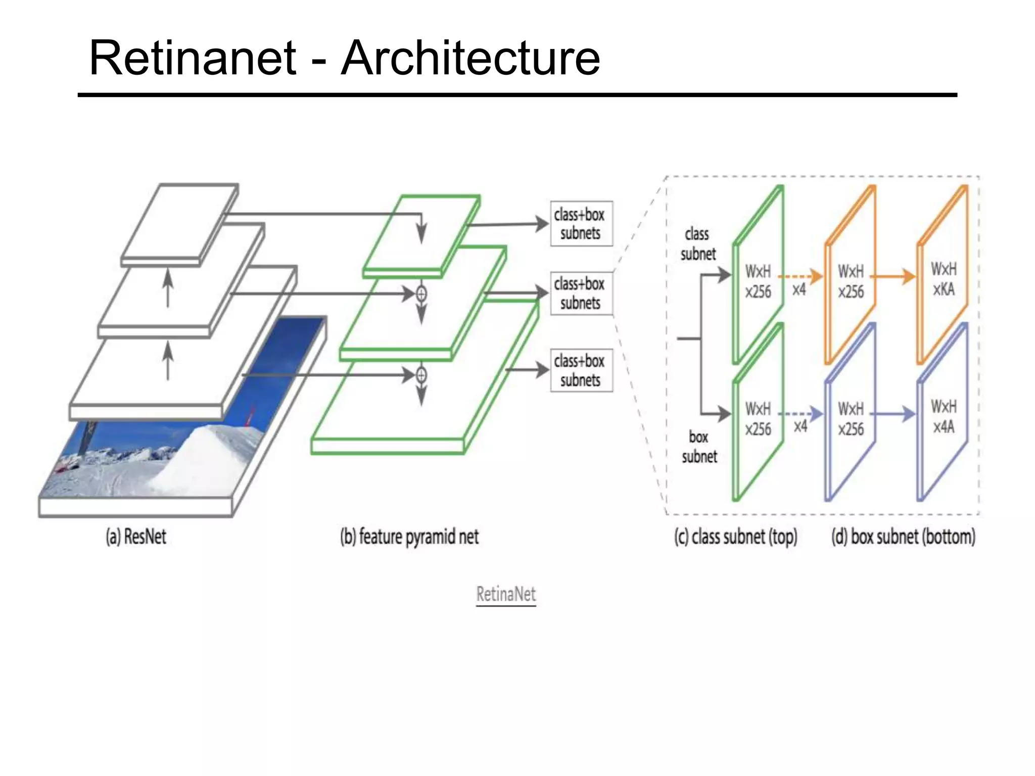
The document discusses various object detection methods, including selective search, R-CNN, and the Fast R-CNN approach, focusing on their advantages and disadvantages related to training time and proposal quality. It highlights the importance of region proposals and introduces the Faster R-CNN, which employs a Region Proposal Network (RPN) for improved proposal generation. Additionally, it covers advancements like Focal Loss and the use of Feature Pyramid Networks (FPN) to enhance detection accuracy across different scales and contexts.
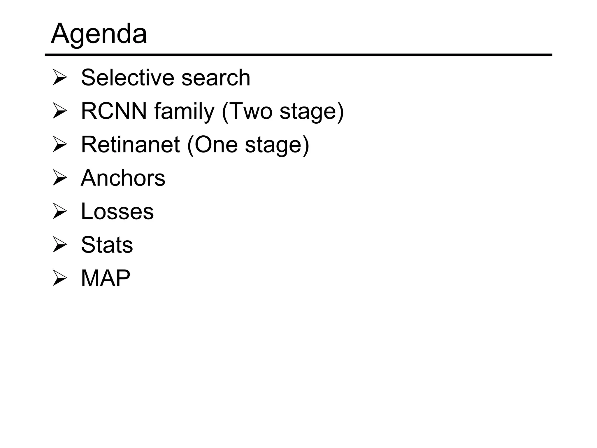
Overview of object detection, agenda includes selective search, RCNN family, Retinanet, anchors, and loss metrics.
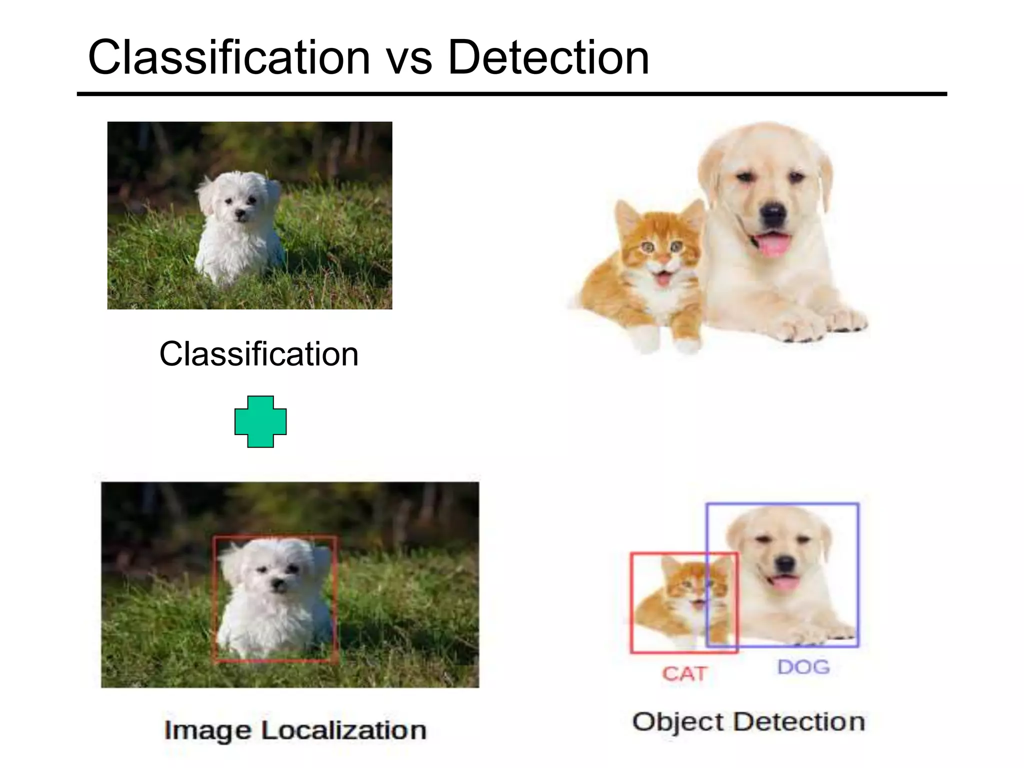
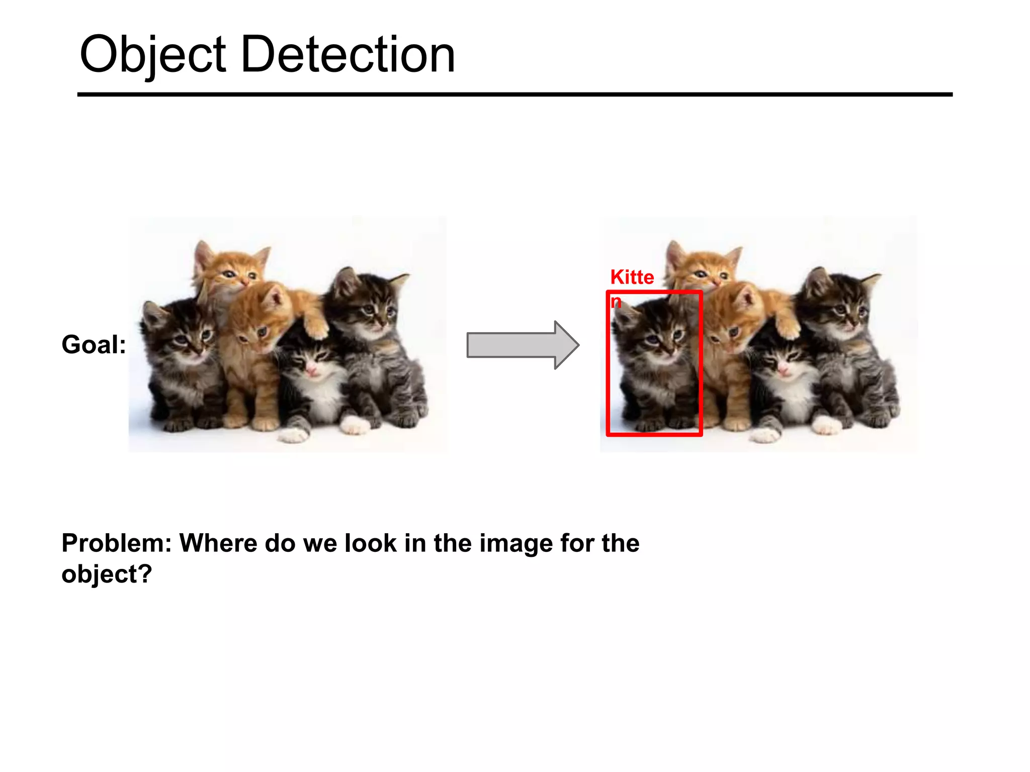
Distinction between classification and detection, focus on where objects are located within images.
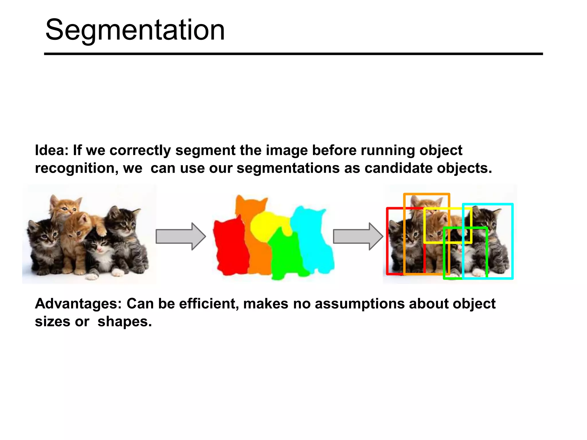
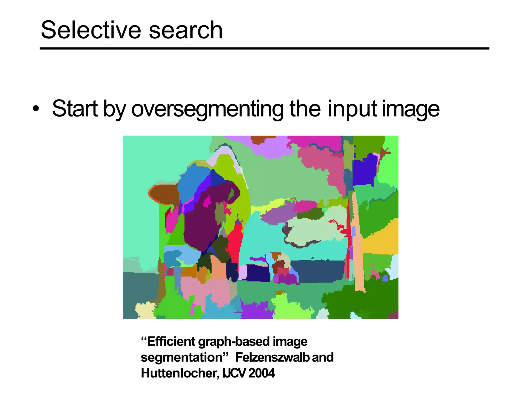
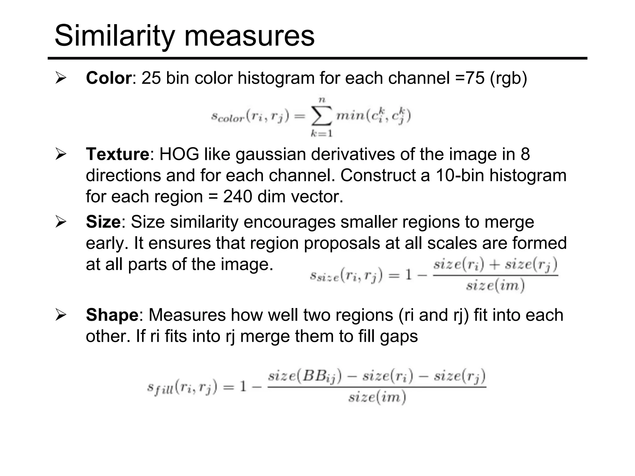
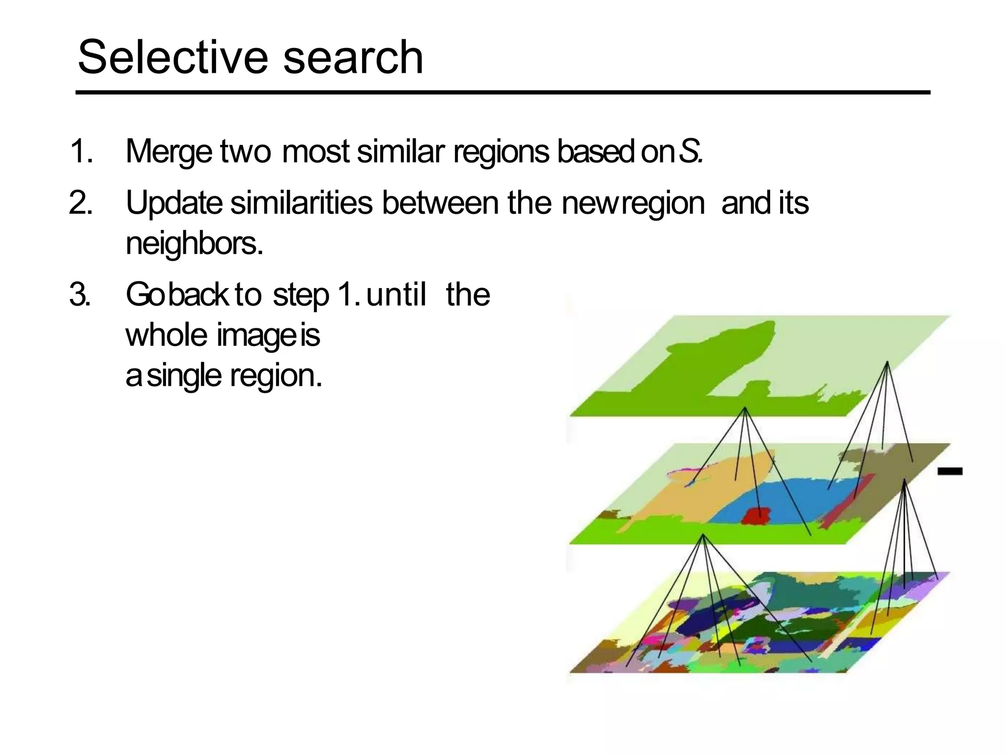
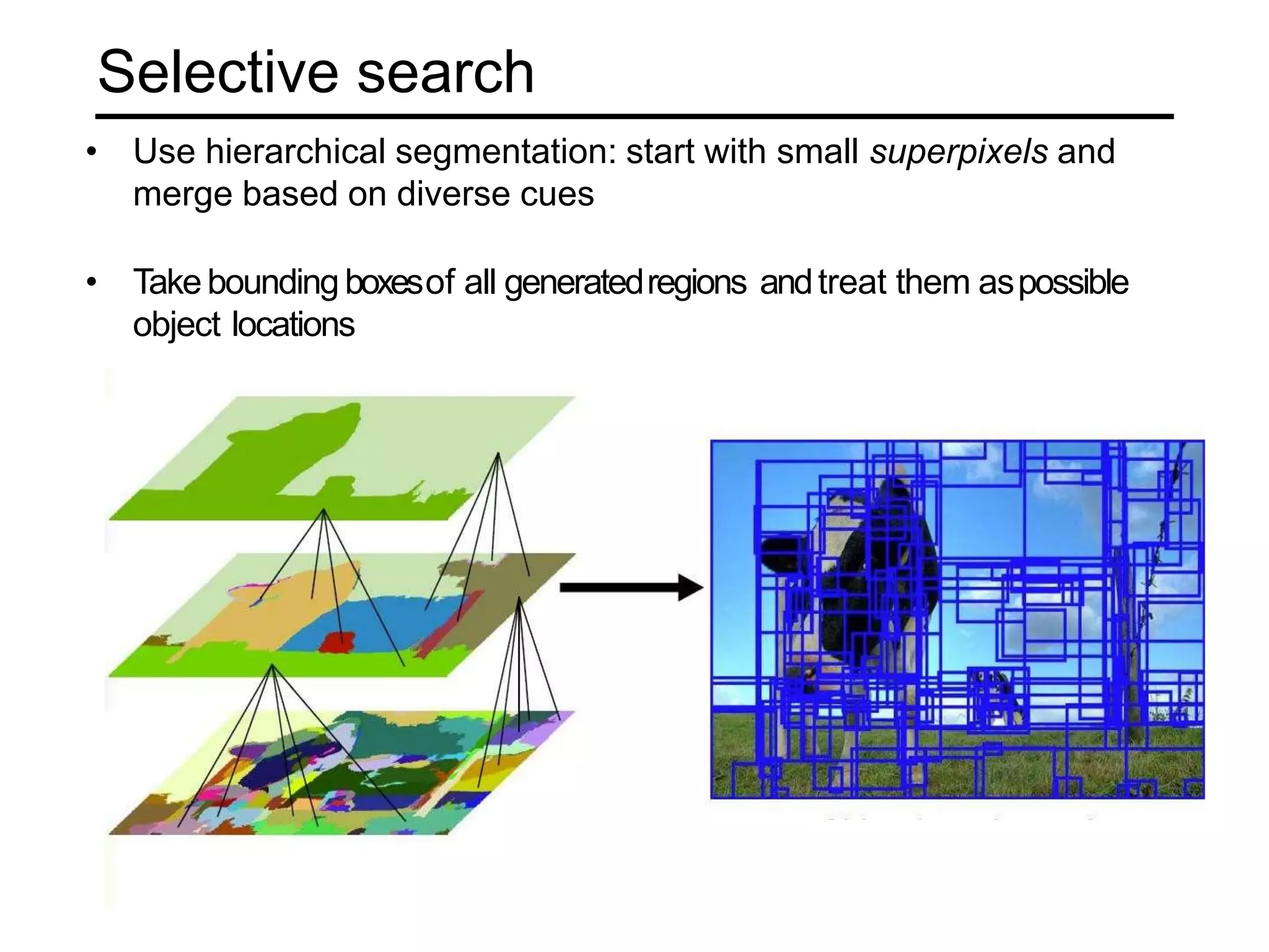
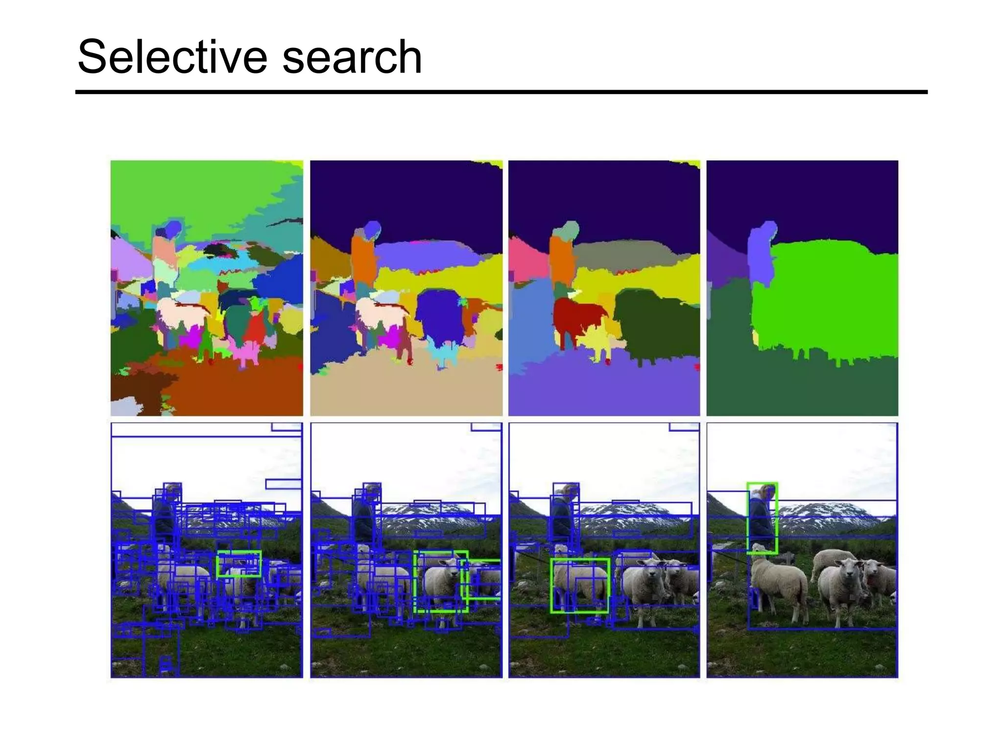
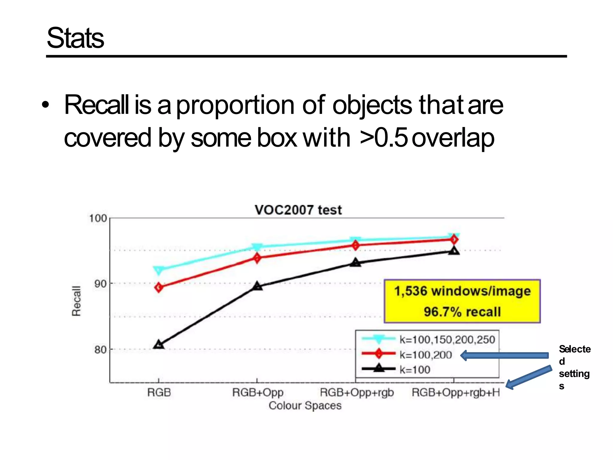
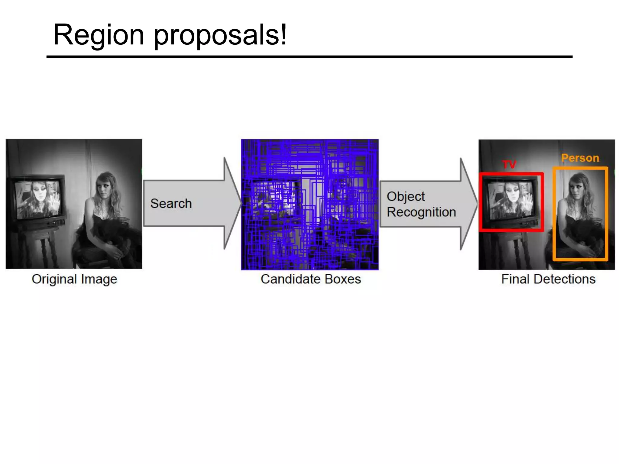
Segmentation by oversegmenting images for efficient object recognition; introduction to selective search for candidate object regions.
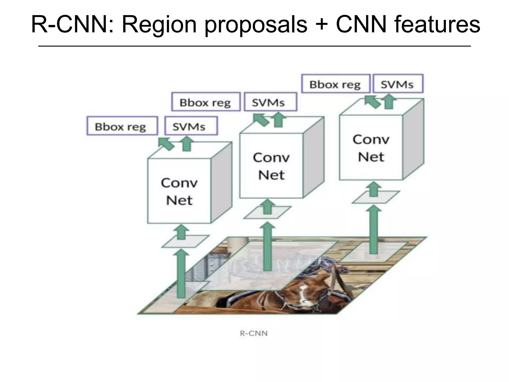
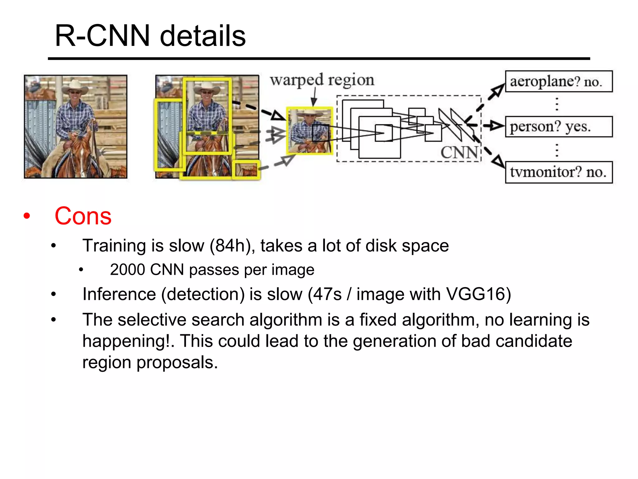
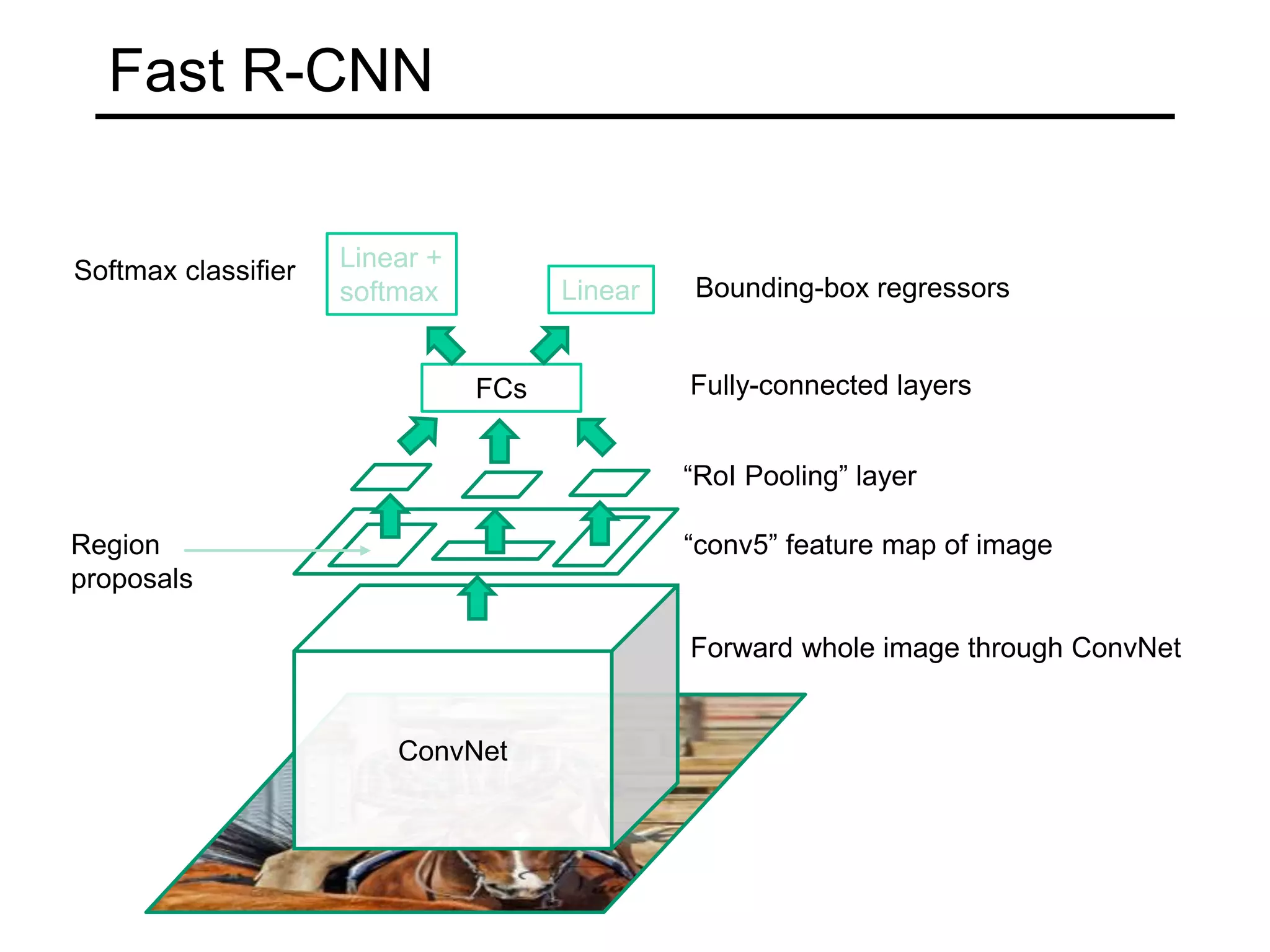
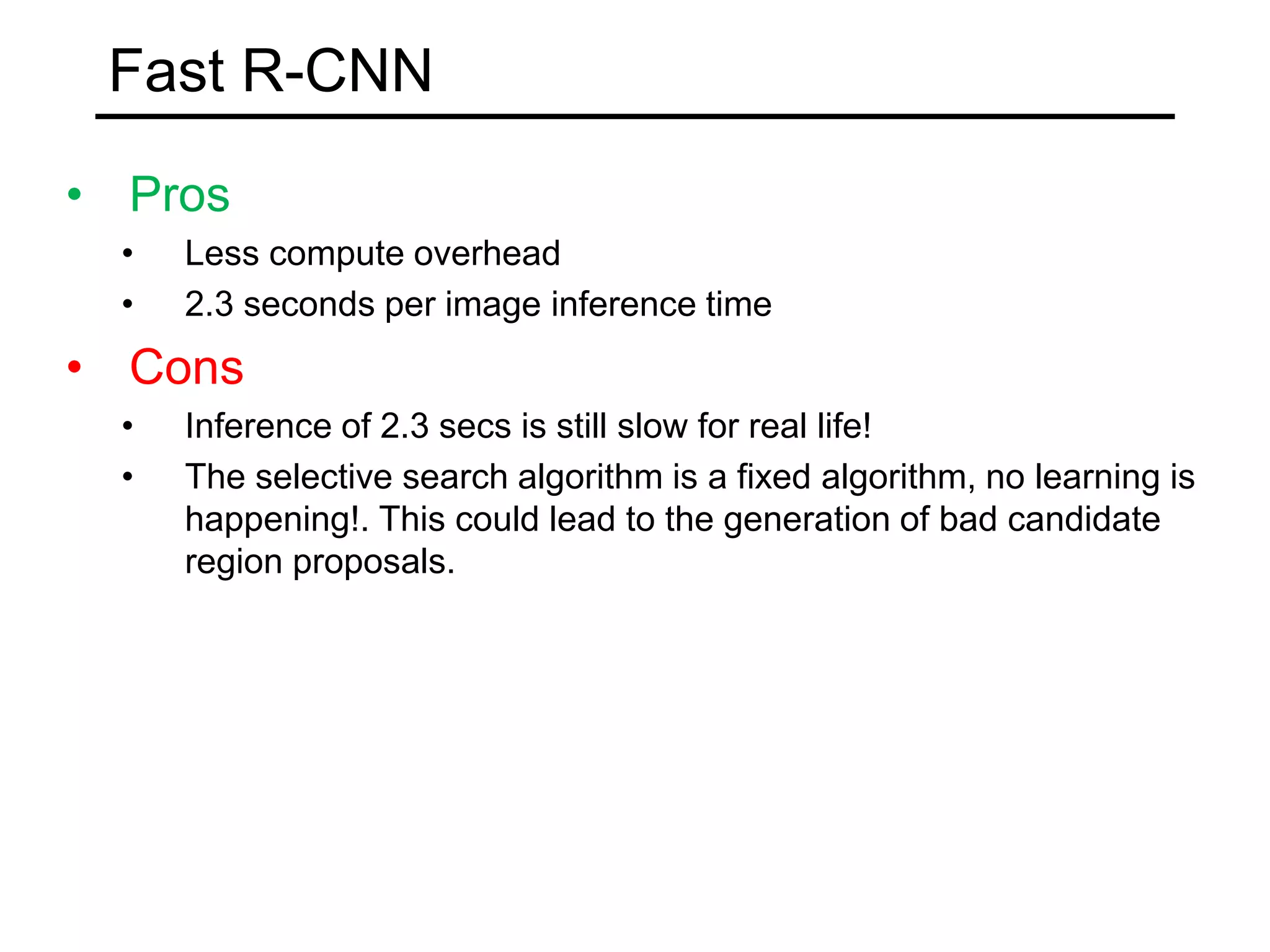
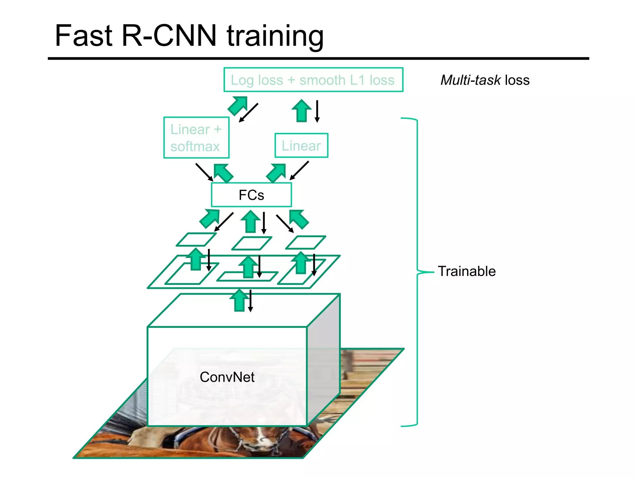
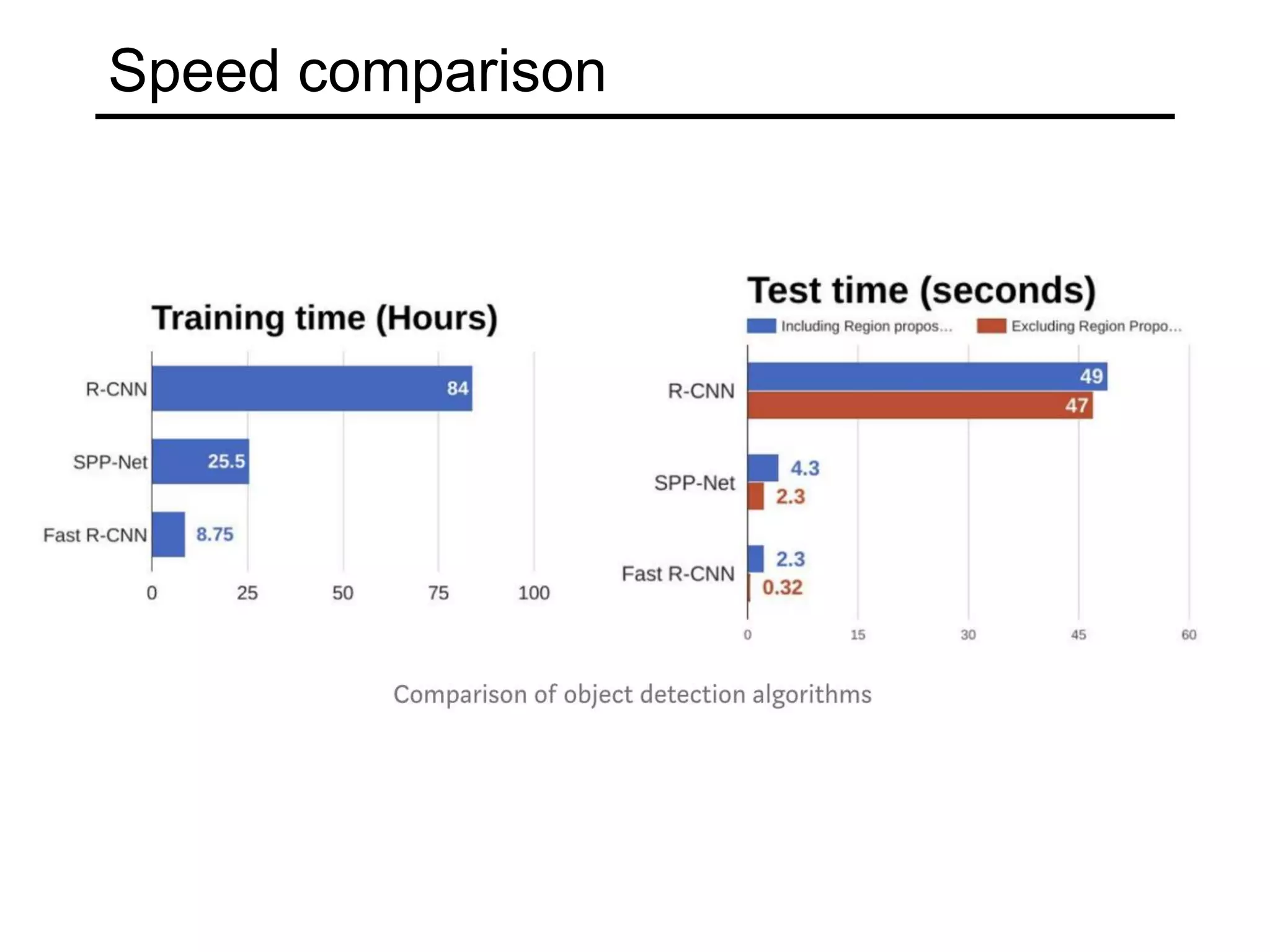
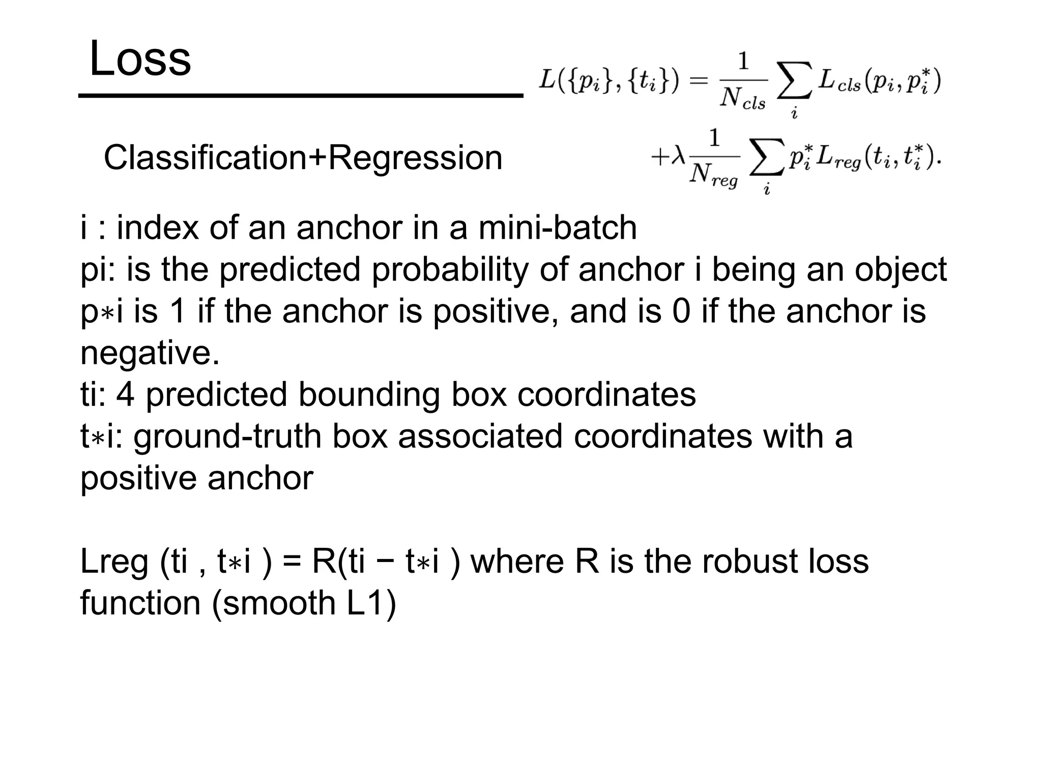
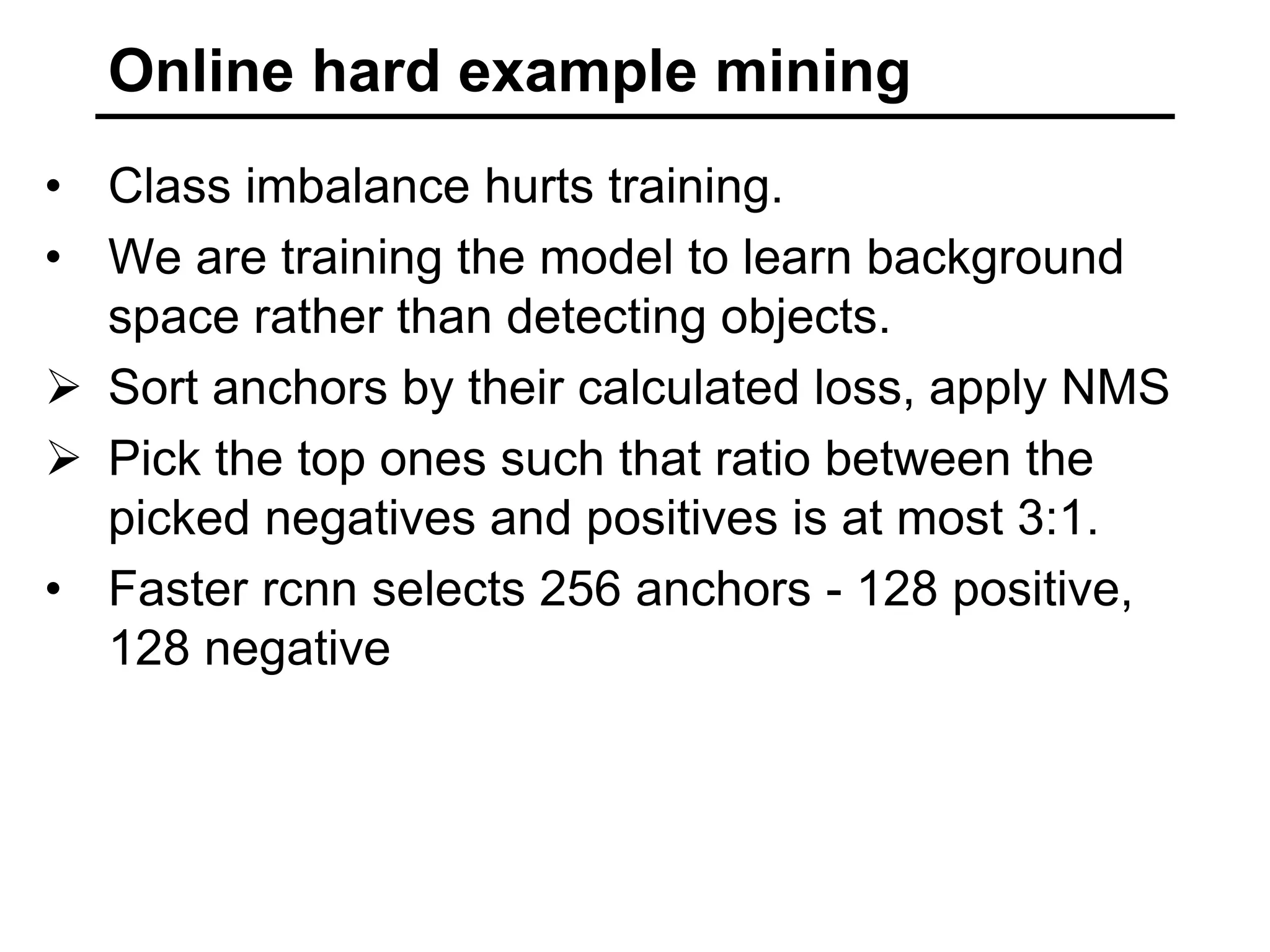
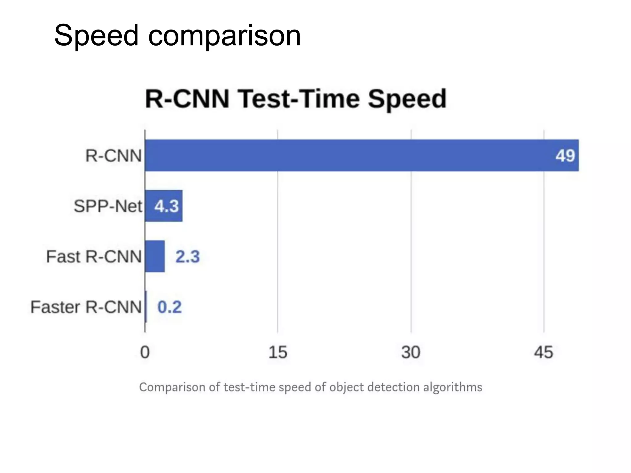
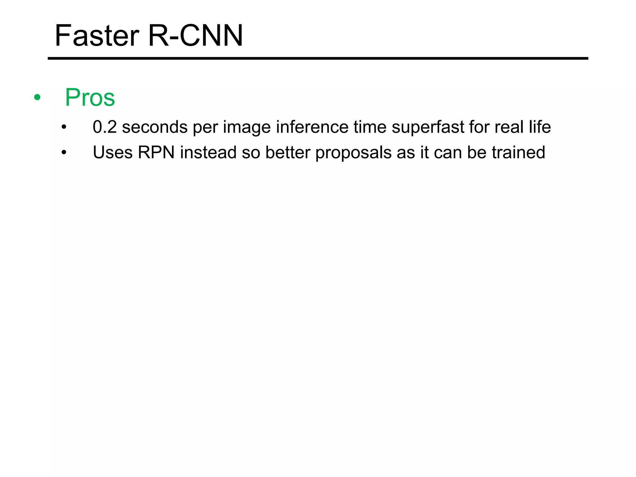
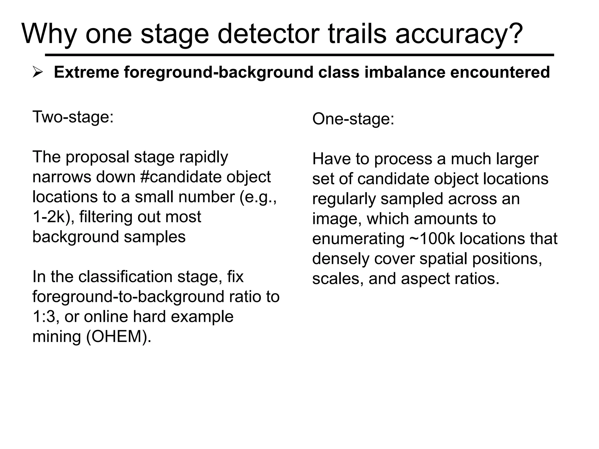
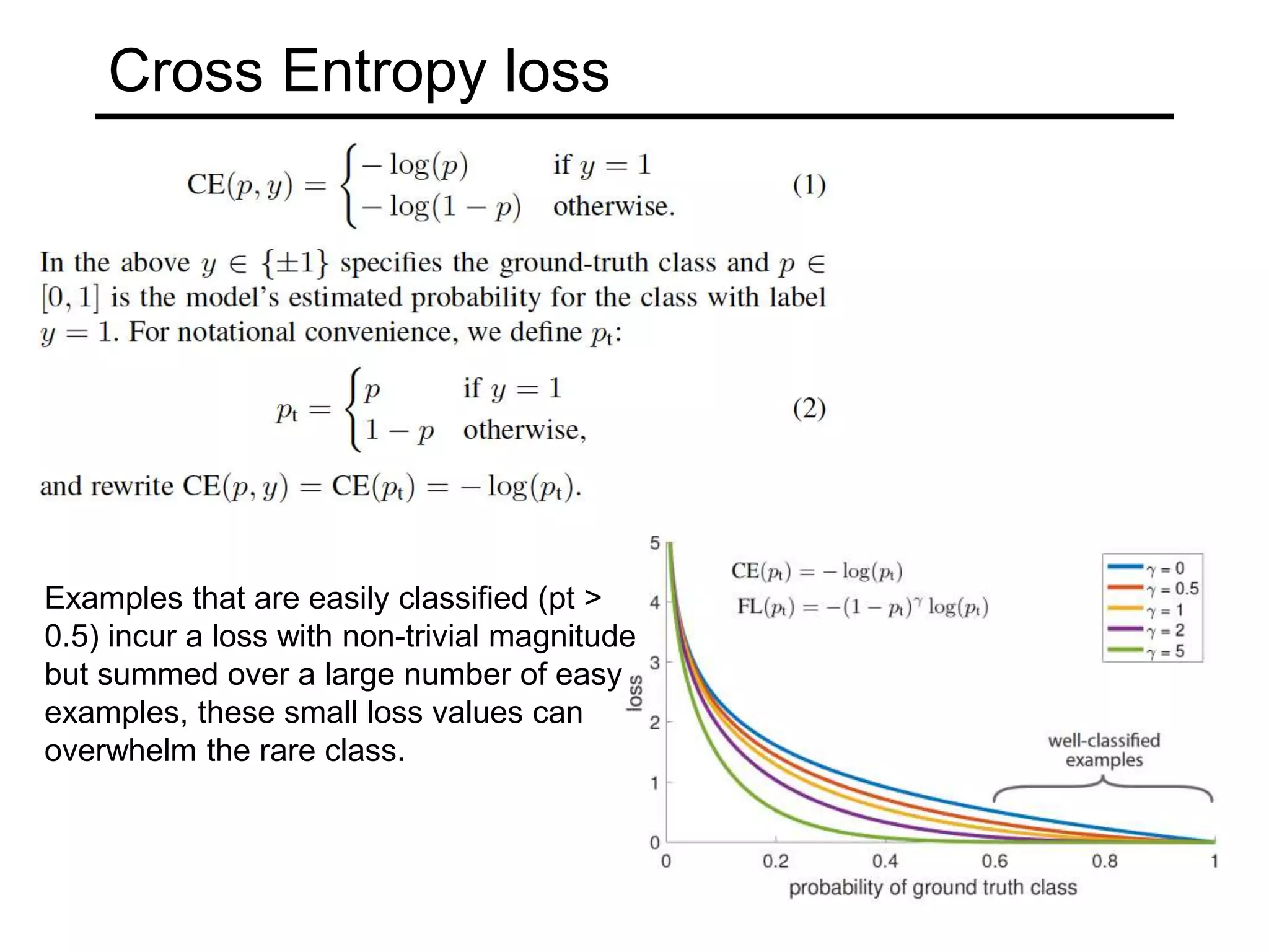
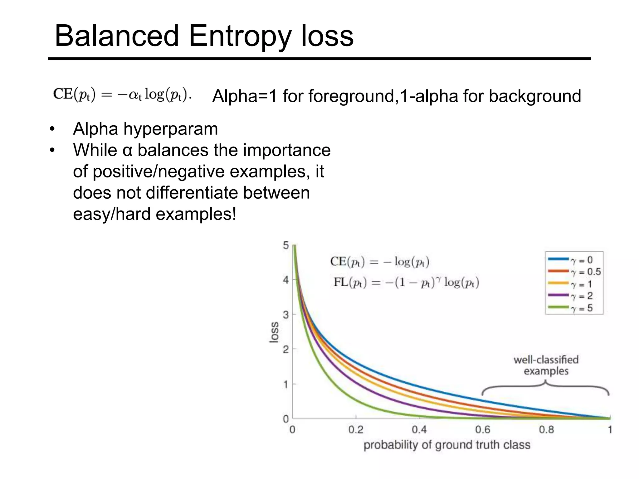
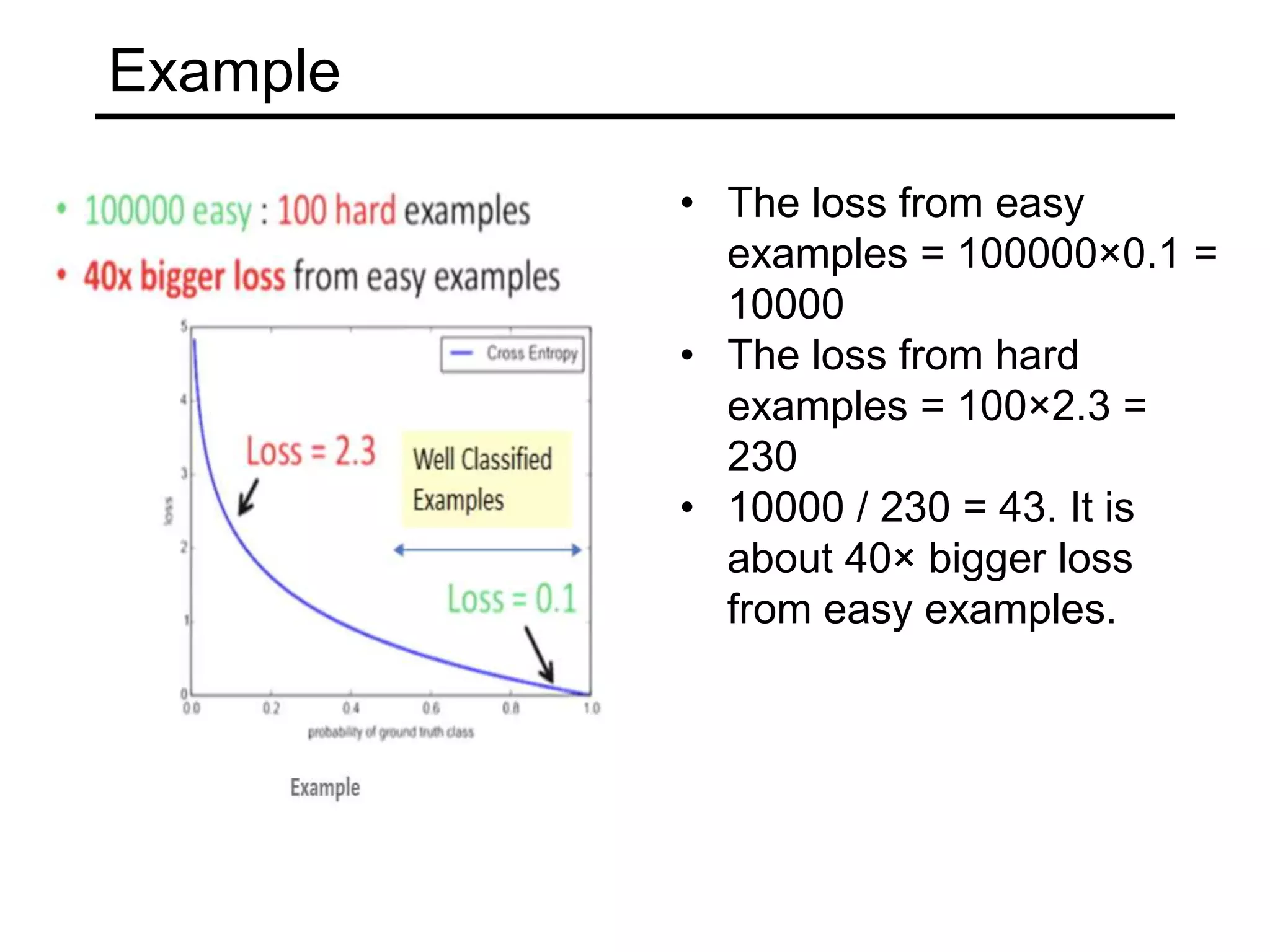
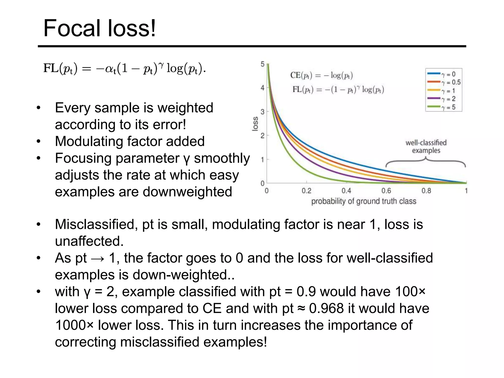
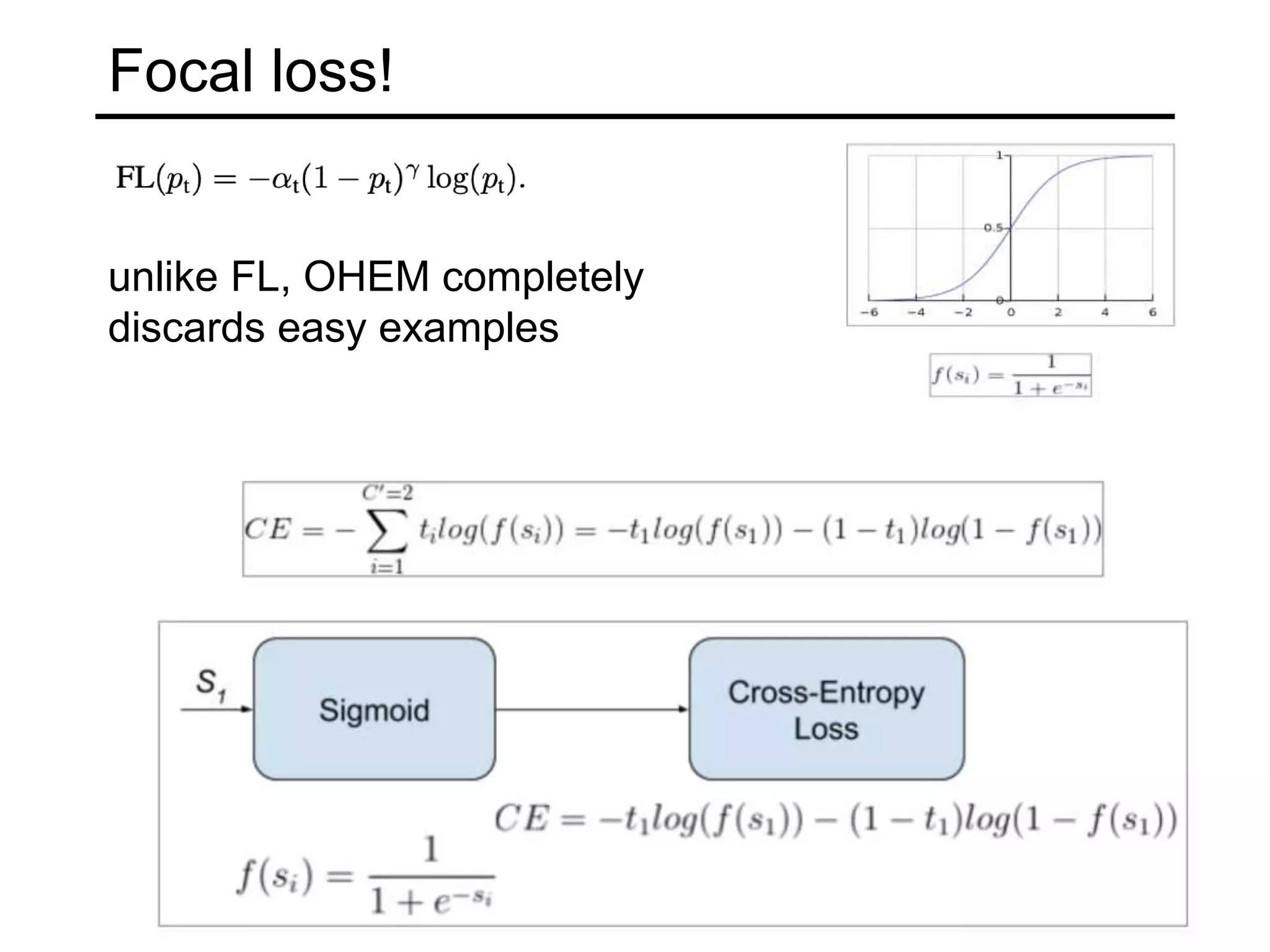
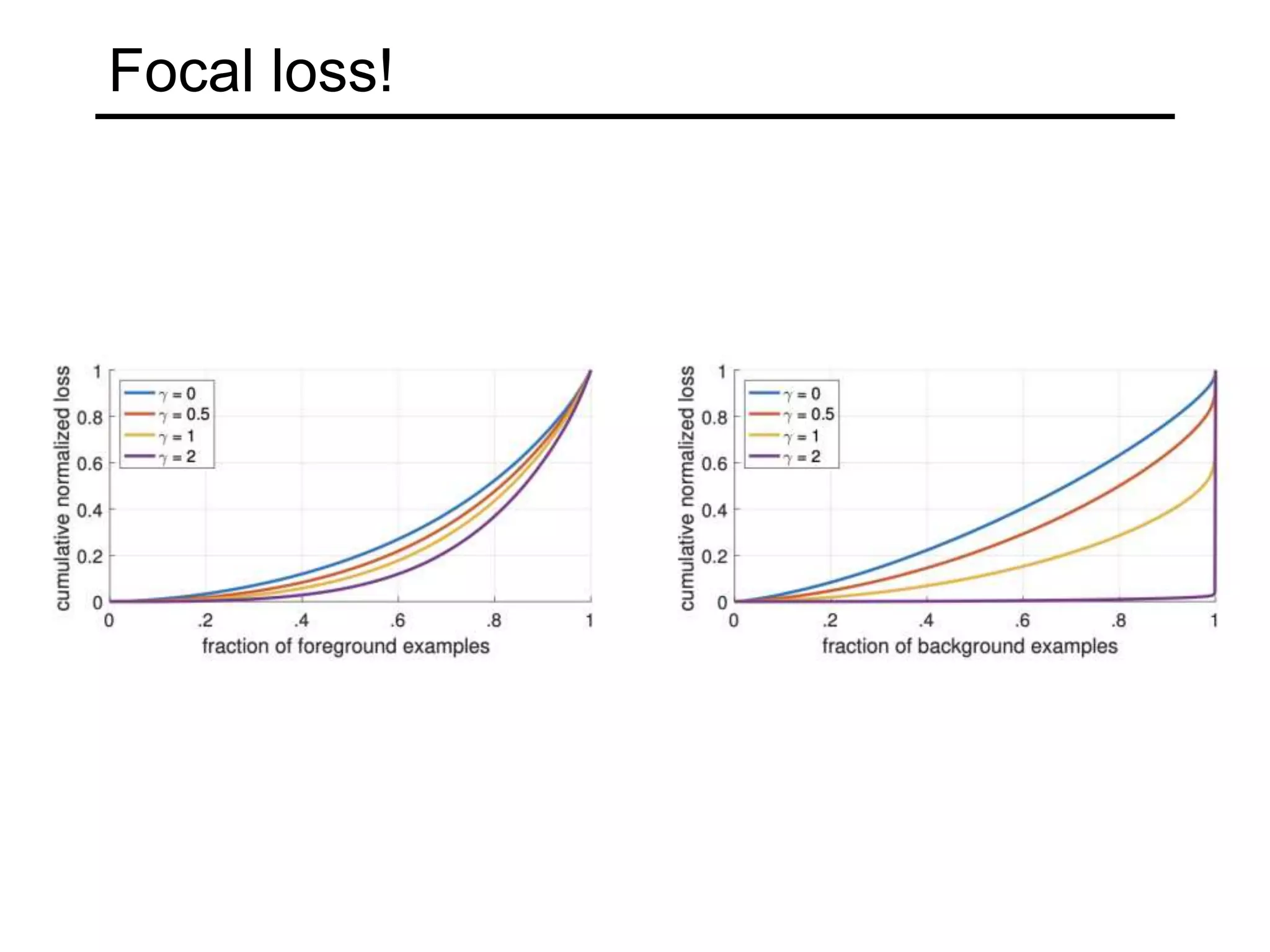
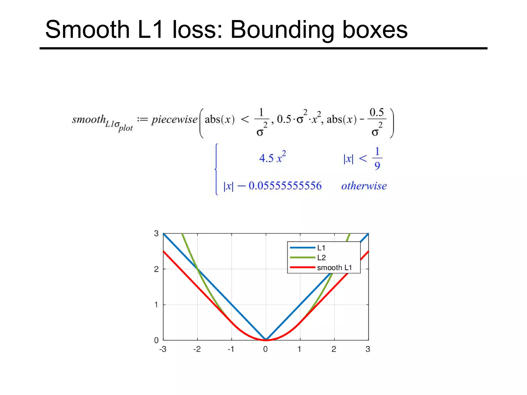
Evolution of R-CNN to Fast R-CNN and Faster R-CNN; highlights region proposals, inference speed, and algorithm limitations. Discussion on loss calculations like cross-entropy, balanced entropy, and focal loss drivers in training, with emphasized importance on misclassified samples.
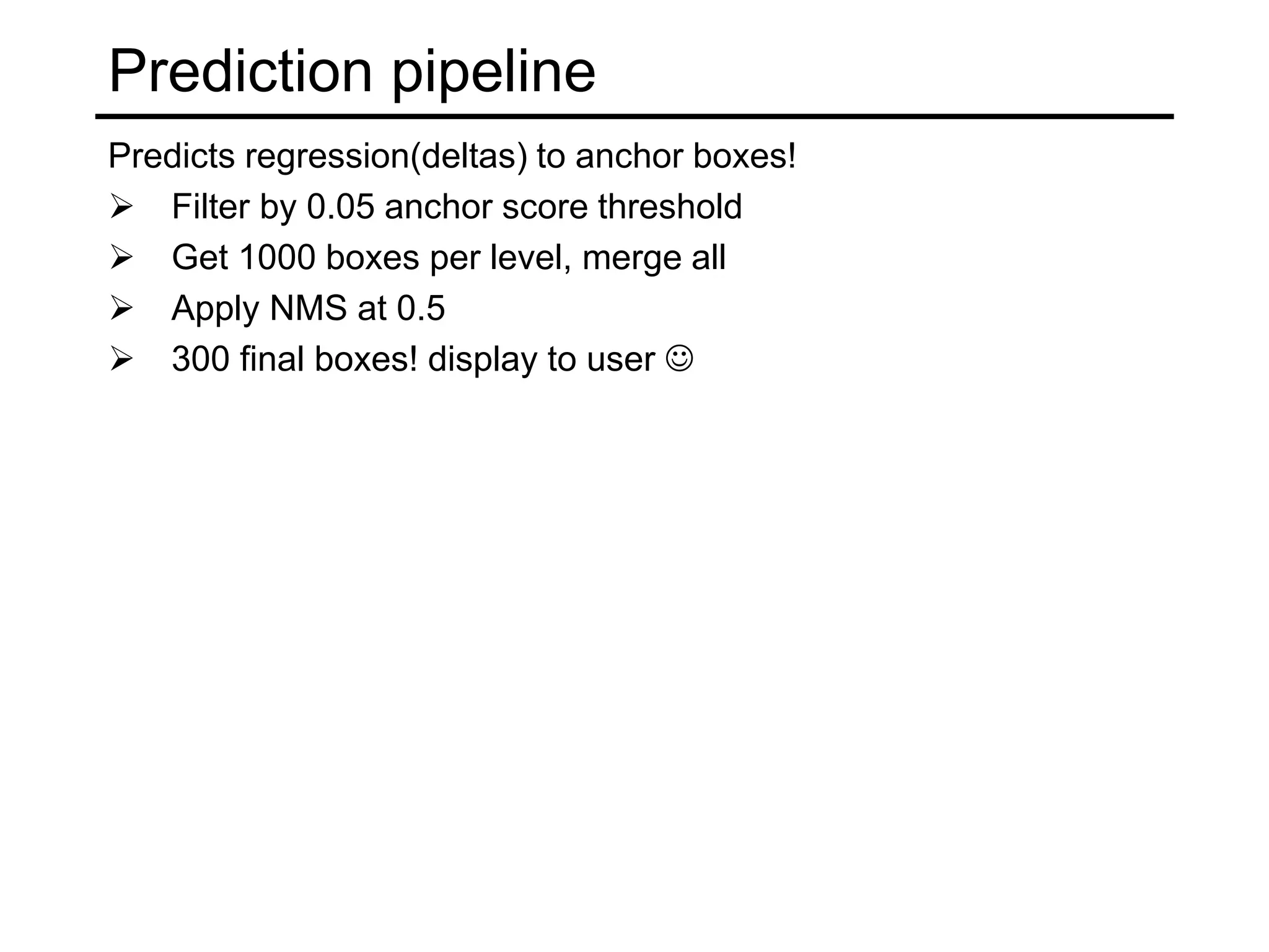
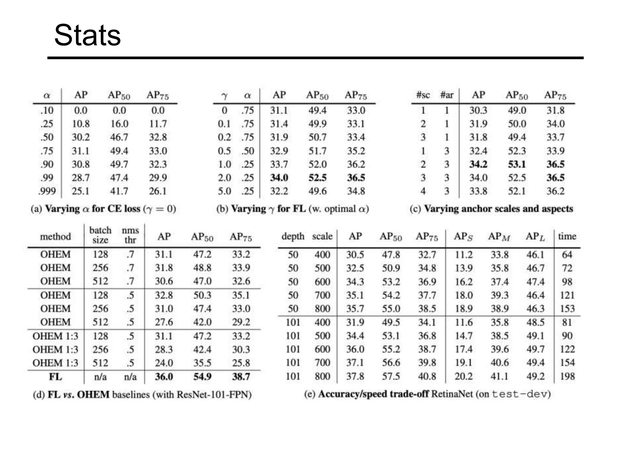
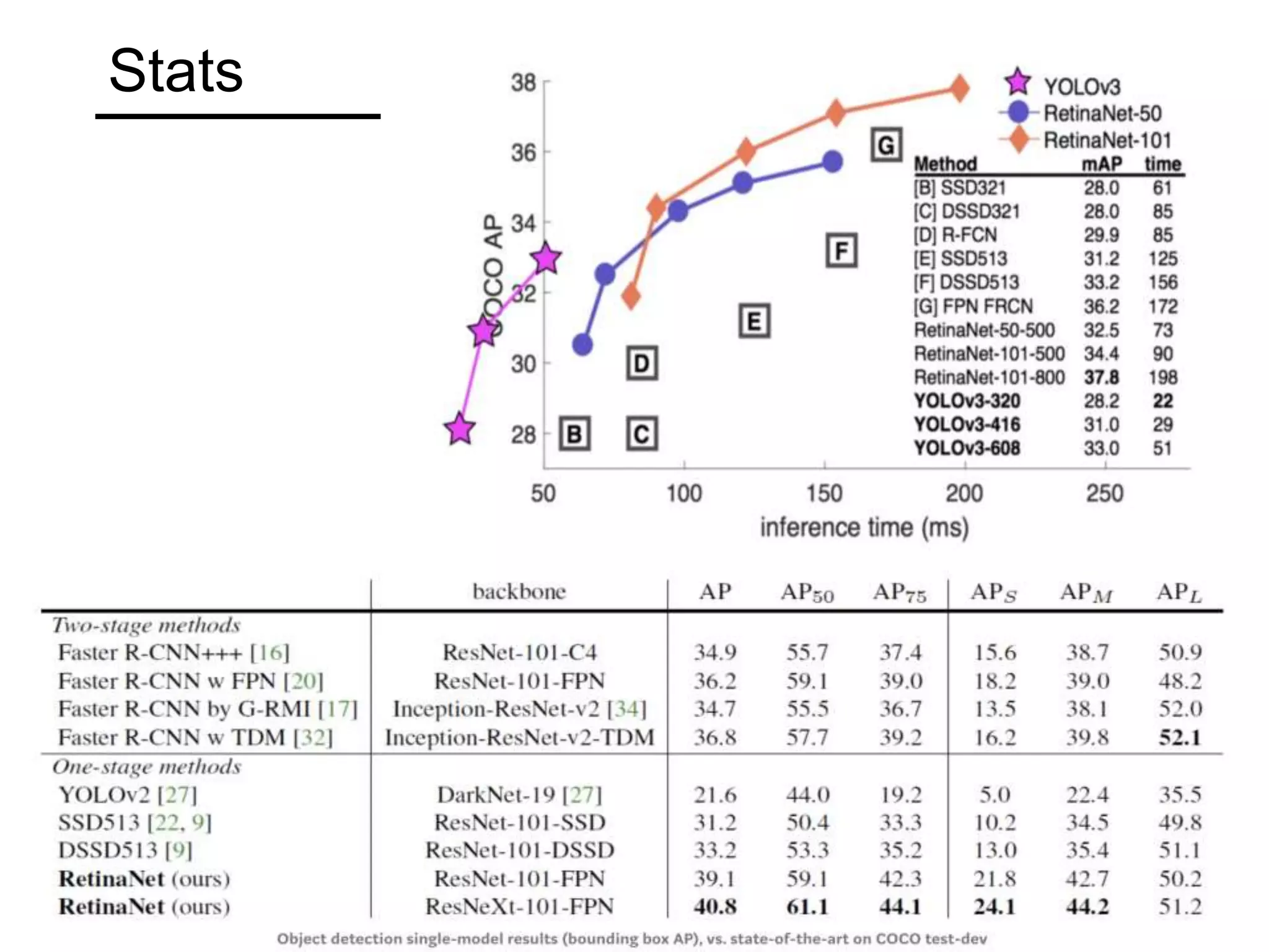
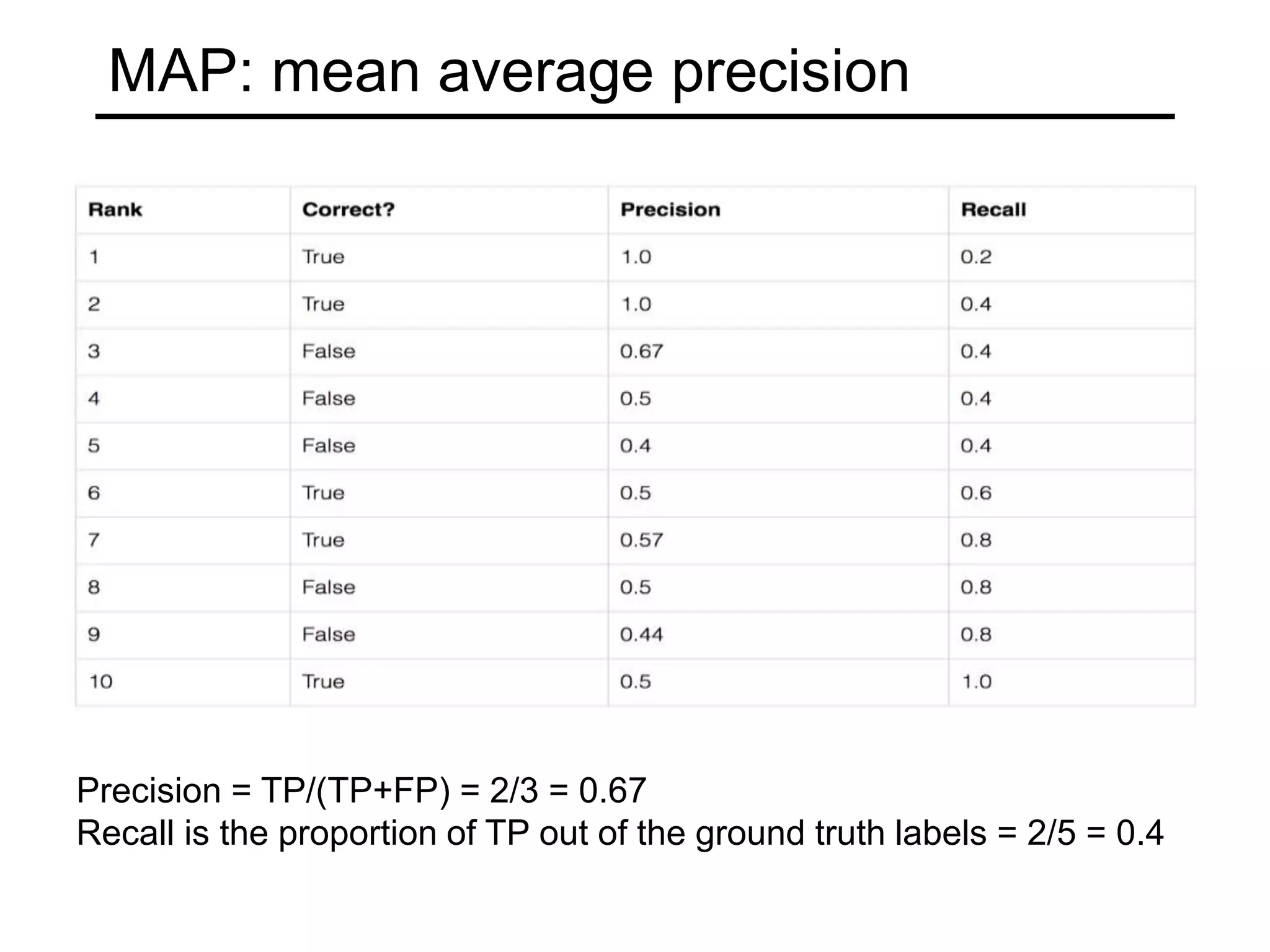
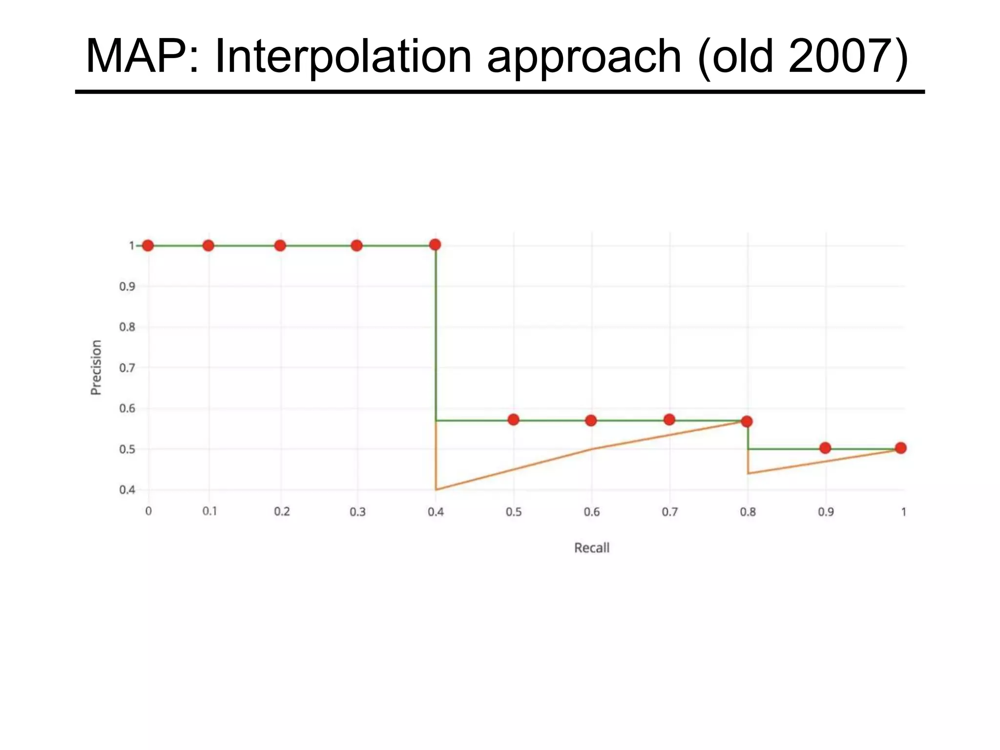
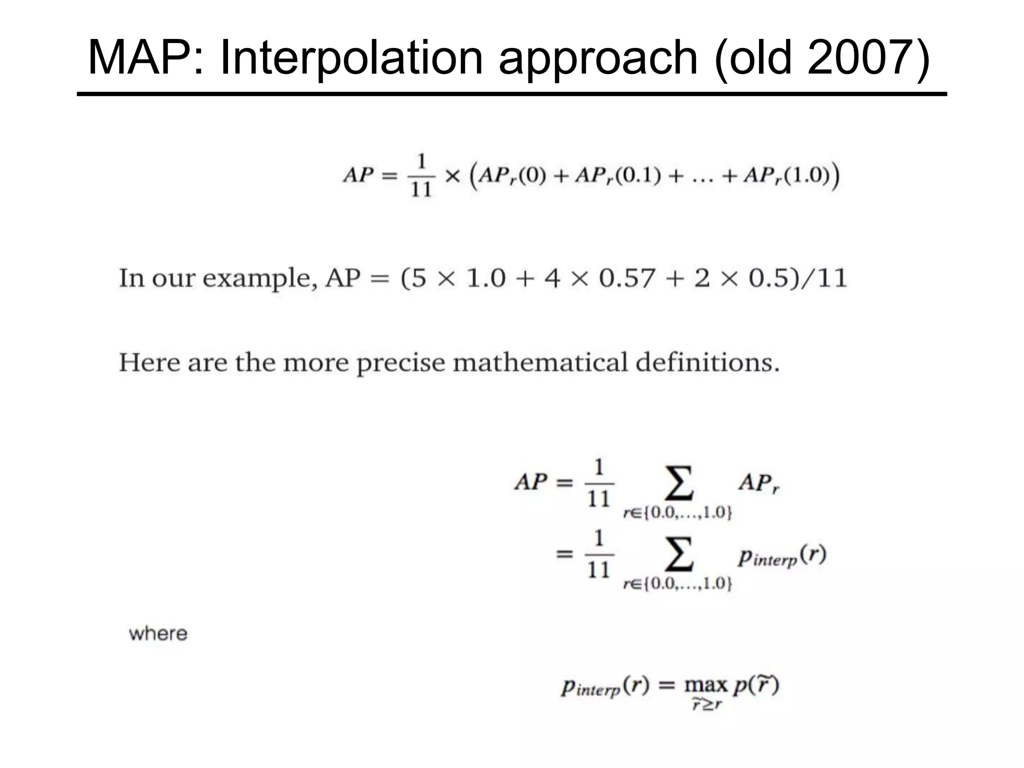
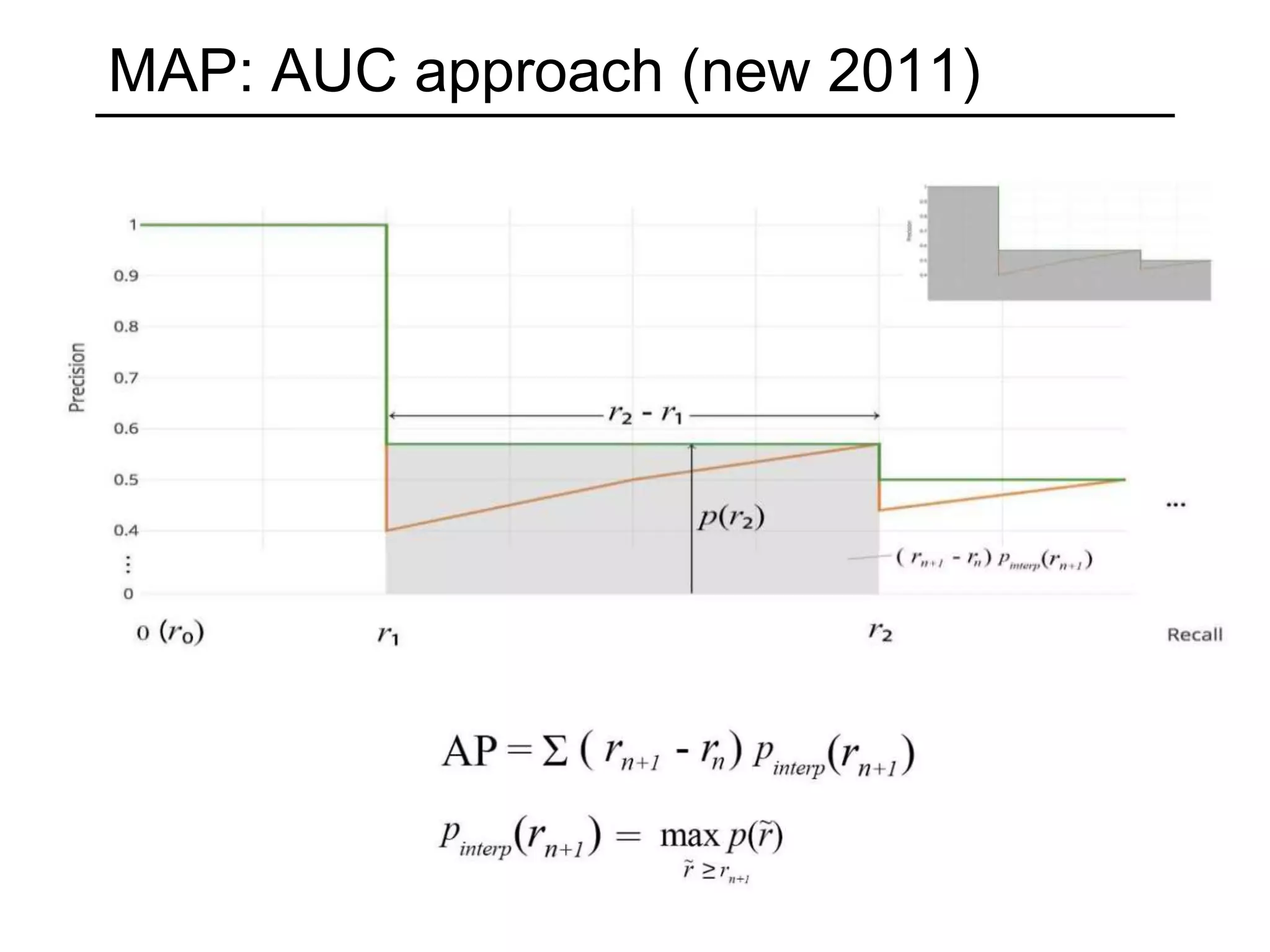
Details on the prediction pipeline and MAP metrics for evaluating model performance, including interpolation and AUC approaches.


![ViT (Vision Transformer) Review [CDM]](https://cdn.slidesharecdn.com/ss_thumbnails/vitreviewcdm-201012184226-thumbnail.jpg?width=640&height=640&fit=bounds)


![Vibe Coding vs. Spec-Driven Development [Free Meetup]](https://cdn.slidesharecdn.com/ss_thumbnails/vibecodingvsspecdrivendevelopment-251209105622-43f455e7-thumbnail.jpg?width=640&height=640&fit=bounds)


