How to Analyze the Results of LinearPrograms—Part 1 Prelimi.docx

How to Analyze the Results of Linear
Programs—Part 1: Preliminaries
HARVEY J. GREENBERG Mathematics Department
University of Colorado at Denver
PO Box 173364
Denver. Colorado 80217-3364
In a four part series, I describe ways to analyze the results of
linear programs beyond what is commonly described in text-
books. My intent is to capture the thought process in analysis
with two objectives. First, I want to provide a guide to those
getting started in applications of linear programming by sug-
gesting useful ways of looking at the results. Second, I want to
help create an artificially intelligent environment for the analy-
sis of results by presenting a protocol that a knowledge engi-
neer can use. The former has been in the folklore for decades;
the latter is part of a project to develop an intelligent mathe-
matical programming system. This first part of the series con-
tains basic terms and concepts used in the other three parts:
price interpretation, infeasibility diagnosis, and forcing
substructures.
A great deal of research and develop-ment activity in large-
scale linear
programming (LP) has been devoted to
solving problems faster. A medium-size
problem by today's standards contains
about 5,000 equations and 20,000 vari-
ables. Even microcomputer versions can
handle thousands of equations and vari-

ables, and supercomputers have been used
for problems with millions of variables!
How can we understand the results? At
one level, in the interests of model man-
agement, we must verify that the solution
obtained makes sense with respect to the
Cupyrighr S) 1993, The Inslilute of Management Sciencos
OO91-21U2/93/23O4/OO56S0I.25
This paptr was refereed.
PROCRAMMENG—LINEAR
INTERFACES 23: 4 July-August 1993 (pp. 56-67)
LINEAR PROGRAMS
problem represented by tho linear pro-
gram.
Once we think we have a good run, we
must delve into the meaning of a solution.
Questions of sensitivity play a direct role,
such as What if . . .? and Why . . .? For
example, we may ask the following. What
if the demand for a commodity increases?
What if capacity is expanded? What if
some resource is made available? Why did
this plant not operate? Why is total pro-
duction so low? Why is the price of some
commodity so large? Why does a certain
flow pattern occur? Is it preferred to others
because of the economic trade-off, or are

the flows forced by the constraints?
Textbook wisdom does not go far
enough in answering these questions in
practical terms (see Gal [1979] for an excel-
lent mathematical treatment). Also, once
an answer is obtained in some mathemati-
cal way, how can we present the answer to
problem owners who might not know lin-
ear programming? We must be able to look
at different views of linear programs and
their pieces, for example, using graphic tech-
niques to present information about flows.
Before we can venture into this world of
analysis, we must understand how linear
programs are constructed. In this overview,
I describe and illustrate some terms, con-
cepts, and principles that one needs to un-
derstand bow to analyze LP results. I have
published earlier tutorials on new ap-
proaches to analysis [Greenberg 1978,
1981, 1982]. The references I give here are
not exhaustive of the attention devoted to
analysis (for an extensive bibliography, see
Greenberg [1992c]).
LP Structure and Syntax
It is important to understand how linear
programs are formulated in order to de-
velop practical analysis techniques
[Williams 1978]. The rules of LP composi-
tion comprise the syntax of the linear pro-
gram.

Mathematically, we use the algebraic
representation, y ^ Ax and L < {x, y) < (J.
Subject to these equations and bounds,
some linear function, like cost, is mini-
mized. I call the A"-variab!es levels of activi-
ties, and 1 call the ly-variables logical levels
because y is determined logically from x
and the equations. The bound constraints
typically have L, > 0 for the level, x,, and
many of the (explicit) upper bounds (L/,)
are infinite for x's. Positive lower bounds
arise to represent minimal levels of opera-
tion or contracted shipments. Finite upper
bounds arise to represent capacity limits of
physical units or market limits of sales.
The canonical form, generally found in
textbooks (for example, Dantzig [1963]), is
to minimize ex subject to AY > b and x > 0.
Bounds can be incorporated into the con-
straints, and free variables (that is, those
allowed tt) be negative) can be partitioned
into their positive and negative parts.
Many different algebraic forms are treated
in most textbooks and shown to be mathe-
matically equivalent to the canonical form.
To reach our form, simply define y = Ax,
set the lower bound of y equal to b, and let
all upper bounds be infinite. Conceptually,
however, it is better to segregate bounds
on variables from equations that represent
relations among the variables.
The coefficient matrix. A, is highly struc-
tured. Often, it decomposes into blocks
with special equations or activities that link

the blocks in a well-formulated linear pro-
gram. For example, the blocks could be
July-August 1993 57
GREENBERG
processes in different regions, and the links
could be aggregate resource limits or trans-
shipment activities. Knowledge of such
structures can be useful in analysis [Baker
1990 and Welch 1987].
Sometimes the structures are known or
can easily be inferred from the model's
syntax—that is, from the rules for compos-
ing the objects and relations that comprise
the LP. Other times, structures are inferred
by executing a recognition algorithm. One
example is recognizing a network embed-
ded in the LP,
Typically, the analysis process has two
steps. First, tbe analyst must work tbrougb
the relevant portions of tbe linear program,
generally witb analytical techniques, to
compute implied relations using the LP
structure. Second, once tbe mathematical
phase of analysis is completed, tbe analyst
must translate the results so that they will
be comprebensible to someone concerned
witb the analysis, generally with linguistic
techniques using tbe LP syntax. Tbis some-
one could be a problem owner for whom

tbe linear program is used, sucb as an en-
gineer or corporate executive. Tbe some-
one could also be a data-base manager
wbo must become involved if questions of
data arise.
In practice, variables tend to fall into
classes. Activity classes can be production,
consumption, transportation, conversion,
capacity expansion, or inventory carrying.
Equation classes can be resource limits, de-
mand requirements, flow balances, or
quality assurance ranges. Tbese lists are
not exhaustive, but typically a linear pro-
gram bas fewer tban a dozen classes of ac-
tivities and even fewer classes of equa-
tions. Wbat makes a linear program large
are tbe dimensions of basic entities, like re-
gions, materials, and time periods [Glover,
Klingman, and Phillips 1990, 1992].
To understand a solution, one must have
a sense of the basic dimensions and classes
of variables. Traditionally, tbe names of
rows and columns in a linear program con-
tain the underlying syntax.
One way to express an LP model, which
is tbe way of most textbooks, is first to de-
fine sets, domains, data tables, and vari-
ables, and second to define the constraints.
To illustrate, I shall explain a production-
distribution model.
Given are
(1) A collection of plants distinguished by

their locations and processes of opera-
tion, wbicb require raw material inputs
and produce finisbed products;
(2) Markets, distinguisbed by tbeir loca-
tions and products; and
(3) Transportation links from plants to
markets.
Tbe data for a specific instance are:
R,,,i = unit amount of raw material i used
by process p at plant j;
Ypjk = unit yield of product k from process
p at plant j;
S, ^ total supply of raw material /';
COST—OPpi = unit operation cost of pro-
cess p at plant j;
K, ^ capacity limit of plant /, measured in
terms of its total output;
COST—SHjnit, ^ unit shipping cost of prod-
uct k from plant; to market
m (if there is no link from
plant ;• to market m for
product k, tbe value of
COST^SHj,,,), = GO); and
D,,,( ^ demand for product k tbat must be
satisfied in market m.

INTERFACES 23:4 58
LINEAR PROGRAMS
The variables are:
Pf,i ^ level of production using process p at
plant /;
T,,,,i = amount of product k sent from plant
/ to market m; and
COST ^ total cost of production and trans-
portation.
The LP model is:
Minimize COST subject to: P,,,, T,,,,̂ > 0;
COST - ^,,i
(Raw material availabihties),
C{/) - XpPp, < Kj (Capacity limits),
B{j. k) - 2,,y,,,P,,, - 2«,T,,,,i - 0
(Balance equations), and
D{m, k) - 2,T,,,,t > D ,̂i (Demands).

Notice that I began with the definition of
sets and data tables. In expressing the
model, I defined each variable with a sym-
bol (P and T) over domains (set products);
then, I wrote the objective and the con-
straints. This is the algebraic form. Alter-
natively, 1 could express the model in
schema form (Figure 1).
In the schema form of the model, the
rows have been classified with COST as the
objective row, and the other row types be-
gin with A, B, C, and D. The activities have
been classified as production (P) and trans-
portation (T). The subscripts in the original
problem definition become domains in this
expression. Each domain is a cross product
of sets, usually restricted to only some of
the many products. For example, the trans-

portation activity has three domain sets:
source (plant), destination (market), and
material (product). The distribution net-
work, however, is usually sparse in that
not every plant ships every product to ev-
ery market.
In our example, the sets are as follows:
(' ^ raw material;
p = process;
/ ^ plant (location);
k = finished product; and
m = market location.
When forming the name of a row or col-
umn, ! distinguish its type by its first char-
acter. Then, I specify its domain member,
but without the parentheses and commas.
For example, consider the transportation
activity T{j, m, k) for the particular plant)

= S (a code for South), the particular mar-
ket m - CH (a code for Chicago), and the
particular finished product /c = T (a code
for table). Then, I name the column
TSCHT. (1 use this name syntax here and I
shall use it in the sequel papers).
Suppose, for example, I specify the fol-
lowing set elements.
i = {S, W}: S means steel, W means wood;
COST
A(i)
B(j, k)
C(j)
D(m, k)
COST_OP(p, j)
R(i, p. j)
Y(p, j , k)
1
T(j. m, k)
COST_SH(j, m, k)
- 1
1

= MIN
< = S(i)
= 0
< = K(j)
> = D(m, k)
Figure 1: The schema form of the production-distribution model
offers an alternative view
from the algebraic form.
July-August 1993 59
GREENBERG
;' ^ {1, 2, 3[: 1 means process 1, 2 means
process 2, 3 means process 3;
j = {N, S]: N means North and S means
South;
m - {DE,CH}: D£ means Denver and CH
means Chicago;
k ^ {C, T]: C means chair and T means
table.
Suppose further that the shipping links are
only those shown in Figure 2,
Then, an equation listing for the particu-
lar linear program is as follows (where d
simply indicates some data value).

Minimize COST subject to:
COST ^ dPlS + d P2N + d P2S
+ d TSCHT + d TNDEC + d TNDET
d PIS + dP3N + d P3S
= d P2N + dP2S + d P3N + d P3S
<d
BNC = d PIN + dPSN - TNCHC
- TNDEC = 0
BNT - d P2N + d P3N - TNDET = 0
BST ^dP2S + d P3S - TSCHT = 0
CS ^ PIS + PIS ^ P3S < d
DCHC = TNCHC > d
DCHT = TSCHT > d
DDEC - TNDEC > d
DDET = TNDET > d
All activity levels > 0.
Consider, for example, the first column,
associated with activity PIN. This is the
name of activity P{p, j) for p = I and /

^ N. It uses steel, so it appears in equation
AS, which is row A{i) for / = S. The activi-
ties that produce with process 2, namely
P2N and P2S, each use wood; and, those
with process 3 use fixed shares of steel and
wood. The capacity equation, CN, limits
the total capacities used by the associated
production activities, PIN, P2N and P3JV.
An equation listing is not always the
best way to view a linear program, es-
pecially when it is large. I shall describe
some alternative views that support
analysis.
Alternative Views of Linear Programs
The most common view of a linear pro-
gram, found in textbooks, is an algebraic
one. It presents a dictionary for what the
data and variables mean, followed by a
system of equatioap that represent con-
straints. The sheer size of today's problems
can make an algebraic view confounding
when one is trying to understand patterns
of relationships.
The entire subject of views has been in-
vestigated elsewhere [Greenberg and
Murphy forthcoming]. Here I consider two
views that have been helpful to me in
Plants Markets
(N)
(S)

DE
CH
Figure 2: Shipping links for an instance of
the production-distribution model connect
the north (/V) and south (S) plants to Denver
(DE) and Chicago {CH). The labels on the arcs
show which products (tables and chairs) each
plant can ship to each city.
INTERFACES 23:4 60
LINEAR PROGRAMS
gaining insight quickly for analysis. The
first is a picture of sign patterns in the LP
matrix, and the second is a directed graph.
Figure 3 shows a picture of the example
product distribution LP. Over the columns,
the activity names are printed vertically,
and the entries are the signs of the nonze-
roes (a blank means the coefficient is zero).
The picture gives us a cognitive view of a
pattern, which is often more useful than
an equation listing.
Computer graphics offer us more oppor-
tunities for visual insights, for example,
graph-based views of activity paths from
production through consumption. Graph-
based views can be obtained from a vari-

ety of fundamental graphs associated with
a linear program (the ones I use here were
developed by several authors [Choobineh
1991; Glover 1983; Glover, Klingman, and
Phillips 1990, 1992; Greenberg 1978;
Schrage 1981]; alternative graphs, based
AS
AW
BNC
BNT
BST
CN
COST
CS
DCHC
DCHT
DDEC
DDET
P P
1 1
N S

+ 4
4
4
4 4
4-
P
2
N
4
4
4
4-
P P
2 3
S N
4
4 4
4

4
4
4
4- 4
4-
P
3
S
4
4
4
4
4-
T
N
C
H
C

-
4
4
T
N
D
E
C
-
4
4-
T
N
D
E
T
-
4

4
T
S
C
H
T
-
4
4
=
=
=
< =
=
> =
> =
> =
4

4
0
D
0
4
MIN
4-
4-
4-
4
4-
Figure 3: A picture of Ihe product distribution
linear program shows the sign pattern for a
relational view.
on the structured modeling formalism,
were given by Geoffrion [1987, 1989], and
those based on graph grammars were
given by Jones [1990, 1991]).
The particular graph that I use in this se-
ries is one that relates activities and equa-
tions [Greenberg 1978], The nodes are the
rows and columns, giving a natural divi-
sion into two node types that makes the

graph bipartite. Each link corresponds to a
nonzero in the coefficient matrix, A. The
picture is a view of the adjacency matrix of
this bipartite graph, where each link ap-
pears as either a plus (+) or a minus (-).
There are two ways to account for sign
patterns; either sign each link or orient it.
The former leads to representations of eco-
nomic correlation, which I do not consider
here (see Greenberg, Lundgren, and
Maybee [1989]), and the latter leads to
flow representations, which I now de-
scribe.
Consider an activity that represents an
exchange, where negative coefficients rep-
resent inputs and positive coefficients rep-
resent outputs. Based on this notion of ac-
tivity I/O, orient an arc from its row node
to its column node if the coefficient is neg-
ative, and from the column node to the
row node if it is positive.
(row i)
(row ()
Aihvily Inpul
A,,>0
[column /]
Activity Outp
»• [column ;]

utput ' ^ '
I call this the fundamental digraph, which
can be used with the syntax to give an al-
ternative view of equations, which com-
prise the rows, and activities, which com-
prise the columns. From the fundamental
digraph, there are two projections that of-
fer insights. These are called the row di-
July-August 1993 61
GREENBERG
graph and tbe column di^^raph.
The row digrapb consists of row nodes
(only), and an arc from one row node to
another means there is at least one activity
with one arc from the first row node, and
one arc into the second. Such arcs tend to
represent flows, where the activity trans-
forms some basic entity that is represented
by the two equations. In the standard
transportation problem, for example, the
entity is a location and the transformation
changes the location of the material that is
transported from location at / to location
atk.
... other nonzeroes.
Activity j creates an arc from row node / to

row node k in the row digraph (entities of i
transformed into entities of k).
The column digraph consists of column
nodes (only), and an arc from one column
node to another means there is at least one
equation that is an output of the first activ-
ity and an input to the second. Such arcs
tend to represent an ordering of the activi-
ties.
:... othernonzeroes.
Equation i creates an arc from column
node j to column node k in the column di-
graph (output of j is input to k).
For an ordinary network, the coefficient
matrix is the usual incidence relation, from
sources to destinations. More generally, in
canonical form, negative coefficients corre-
spond to activity inputs and positive coeffi-
cients to outputs. When an activity has
more than one input or more than one
output, the LP is sometimes called a net-
form [Glover 1983] and sometimes called a
process network [Chinneck 1990].
For example, consider the following
2 X 3 system.
S - 2P - T and
D = {T - C.

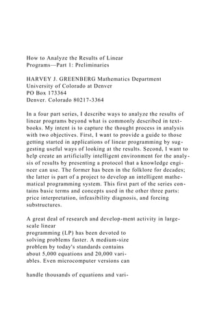
Think of P, T, and C as production, trans-
portation, and consumption activities, re-
spectively; and think of S and D as supply
and demand stocks. For example, suppose
we produce one unit, transport two units
and consume one unit; that is, P ^ 1, T ^
2, and C - 1. Then, S - D - 0; that is, the
stocks are balanced (no excess or shortage).
Figure 4 shows all three digraphs for this
2 X 3 system.
The row digraph shows flow from sup-
ply (S) to demand (D), The column digraph
shows a precedence, where production (P)
precedes transportation (T), which pre-
cedes consumption (C).
1 can also apply these digraphs to por-
tions of an LP, for example, to the portion
of the product distribution LP (compare
Figure 3) that is shown in Figure 5. This
digraph represents a portion pertaining to
demand for tables in Denver (row node
DDET). The headless arc out of row node
DDET denotes a demand requirement, and
the tailless arcs into row nodes AW and CN
denote availabilities of wood and capacity,
respectively.
Figure 6 shows the row and column di-
graphs associated with the fundamental
INTERFACES 23:4 62

LINEAR PROGRAMS
(S)
(D)
[P]
[T]
•[C]
[P]
(S)
I
(D)
[T]
I
[C]
Fundamental Row Column
Digraph Digraph Digraph
Figure 4: The digraphs for the 2 x 3 system
show flows and activity precedence.
digraph in Figure 5. The row digraph gives
a view of flows: wood {AW) and capacity
in the North (CN) are transformed into a
table in the North (BNT), which is trans-
ported to Denver (DDET). The column di-
graph gives a view of activity sequence:

produce a table in the North by process 2
[P2N], then transport the table to Denver
[TNDET].
Re-organization of Equations
In any system of equations, such as y
= Ax, I regard the variables on the right (x)
as independent and those on the left (y) as
dependent. In linear programming, the ter-
minology given to dependent variables is
basic and to independent variables is non-
basic, and these roles oi variables can
change from the original expression to a
form that results from a solution. This
change of role is important to analysis
questions because the dependence of y, on
X, is no longer measured by the original
coefficient, A,,, and dependencies among
the x-variables become revealed by the re-
organization.
(AW)
(CN)
[P2N] (BNT)
For example, consider the 2 X 3 system.
In its original form, we can make such
statements as the following:
—An increase in production (P) causes an
increase in supply stock (S) at double the
rate;
—̂A decrease in transportation (T) causes

an equal increase in supply stock (S) and
a decrease in demand stock (D) at half
the rate.
Notice that the causality is from the in-
dependent variable (on the right) to the
dependent variable (on the left). An alge-
braically equivalent system of equations is
obtained by rewriting the original ones, for
example, the following:
P= ^,S+ jTand
C - {T -D.
In this form, I have kept T as an inde-
pendent variable on the right-hand side,
but I exchanged P for S in the first equa-
tion and C for D in the second. Now P and
C are dependent, or basic, variables, and S
and D are independent, or nonbasic, vari-
ables.
In this form, we can make such state-
ments as the following:
—An increase in supply stock (S) causes an
increase in production (P) at half the
rate;
—A decrease in transportation (7) causes a
decrease in both production (P) and con-
sumption (C), each at half the rate.
The roles the variables assume in any re-
organization of the equations determine

•• [TNDET] • • (DDET)
Figure 5: The fundamental digraph for a portion of the product
distribution LP traces a path
from production to demand.
July-August 1993 63
GREENBERG
(BNT) (DDET) [P2N] [TNDET]
(a) Row Digraph (b) Column Digraph
Figure 6: Row and column digraphs for the portion of the
product distribution LP shown in
Figure 5 show flows and the activity sequence associated with
the flow trace.
causality relationships: what happens to
the dependent, or basic, variable when an
independent, or nonbasic, variable is
changed. The details of how one obtains
the new system of equations from the orig-
inal system are a matter of computation,
and I do not consider them here. What is
important is to recognize marginal rates of
substitution that depend upon the parti,cu-
lar roles, basic versus nonbasic, which is
part of the solution information.
Let us consider an example of how this
information is used for an analysis ques-

tion. Suppose a solution to the product dis-
tribution LP has activities P2N and TNDET
basic, and activity P3JV nonbasic (at its
lower bound of zero). Note, from Figure 3,
that P3N is a substitute for activity P2N~
that is, they are substitutes, or competitors,
because they use the same inputs (wood
and capacity), and they produce the same
output (tables in the North). Activity P3N
uses an additional input (steel) and pro-
duces an additional output (chairs in the
North). The question is. What if activity
P3N were forced to increase to a positive
level?
Figure 7 shows some rates of substitu-
tion, using hypothetical data. Among the
basic variables affected is P2N, whose level
is displaced one-for-one—that is, for each
unit increase in P3N, there is a unit de-
crease in P2N. The level of row AS in-
creases at a rate of 0.4 because activity
P3N uses 0.4 units of steel for each table it
produces (hypothetically). The net effect
on wood used (row AW) is a decrease at a
rate of 0.4 because P3N uses 0.6 units of
wood to produce one table, while P2iV
uses one unit of wood to produce a table;
the displacement of P'5N for P2N results in
a net decrease of 0.4 units of wood per
unit of P3N. The COST row is also af-
fected, where each unit of increase in P3N
results in an increase of $9.00.
Other basic variables are affected by an

increase in P3N, such as the increase in the
level of transportation of chairs produced
by P3N with accompanying displacements
of other chair transportation and produc-
tion.
The rates of substitution can be ob-
tained, but one must take care in interpret-
ing their meaning in the presence of a
property called degeneracy. Although 1
AS = current level + 0.4P3N
+ other non-basic rates
AW = current level - 0AP3N
COST - current level + 9P3/V
P2N = current level - P3N
Figure 7: Rates of substitution, from a rewrite
of the equations, reveal how a change in the
level of activity P3N affects basic variables.
INTERFACES 23:4 64
LINEAR PROGRAMS

shall not consider it in detail here, degen-
eracy will arise in some of our exercises in
the sequels. One form of degeneracy,
which affects the use of rates for sensitivity
questions, occurs when the level of a basic
variable is at its bound, such as zero.
When that is the case, additional analysis
is required to address what-if questions.
The information obtained from rates of
substitution directly addresses not only the
paradigm what if . . .? sensitivity ques-
tion, but also other questions of analysis,
such as the meaning of redundancy in the
interests of model management and deeper
understanding of the results.
The Analysis Processes
I conclude our preliminaries with an
overview of the analysis process. Three
types of analysis processes are (1) validity
testing, (2) postoptimal analysis, and (3)
debugging. Validity pertains to how well
the LP represents the world it is intended
to, but I include, in validity testing, ele-
ments of verification: whether what is in
the LP is what is believed to be there. Post-
optimal analysis is probing into the mean-
ing of an optimal solution. This includes
conventional questions of sensitivity, and it
includes some additional analyses that are
unconventional in the sense that they go
beyond textbook definitions. Debugging is
the process of diagnosing the cause of a
failure, for example, an infeasible LP.

The first thing one checks after a solver
has terminated is whether an optimal solu-
tion has been found. It could be that the
solver detected that the linear program is
infeasible or unbounded. This is called a
mechanical failure, and its detection
launches an analysis effort to diagnose the
cause in order to repair it.
Diagnosing the cause of a mechanical
failure is sometimes called debugging. De-
bugging also applies more generally to op-
timal linear programs, such as checking
that the results make sense. To make
sense, one must explain the results in
problem domain terms. Failure to do so
can lead to erroneous conclusions.
Once we have a run that is not a me-
chanical failure, we check some things that
are particular to the model, and I call this
validity testing. One case that occurred had
the following result. All the variables were
zero, contrary to what makes sense for the
problem. 1 discovered that demands were
inadvertently omitted from the scenario
specification, so a do-nothing solution had
minimum cost. This was easy to detect and
remedy just by looking at the right-hand
sides of the equations.
Other validity tests are not as easy, but
part of the maturation of a model is the
maturation of the personnel that run it.
The tests can become increasingly complex

with this maturation, so what comprises
the vahdity test depends upon accumu-
lated experiences with what can go wrong.
A deep validity test, for example, is to
impute price elasticities from scenarios.
This measures how quantities change with
respect to percentage changes in prices.
Suppose one has a sense that the price
elasticity of a product is about 10 per-
cent—that is, if the price doubles, the pro-
duction is expected to increase by 10 per-
cent. If the imputed value is more like 100
percent, something might be wrong with
the run. (To compute an elasticity, there
must be some other run, such as a base
case, against which to compare the cur-
rent run.)
July-August 1993 65
GREENBERG
In general, a validity test is a test of so-
lution values with a sense of what they
should be. The test looks for gross devia-
tions from the expected results. This is part
of model management, and it has so far
been passed on from one generation to an-
other by on-the-job training. The time is
undoubtedly right for an in-depth treat-
ment of applied Hnear programming that
includes a substantive description of model
management.

In sequels to this overview 1 shall pre-
sent the following examples of analysis.
—Price interpretation: What a dual price
means.
—Infeasibitity diagnosis: Why a mechani-
cal failure occurred.
—Forcing substructures: Separating eco-
nomic trade-offs from forced values.
Collectively, these illustrate some princi-
ples that have been used in practice and
some new ones introduced with the avail-
ability of ANALYZE [Greenberg 1983,
1987, 1988, 1989, 1992a, 1993], a software
system designed to provide computer-
assisted analysis, including rule-based
intelligence.
Acknowledgments
I gratefully acknowledge encouragement
and technical help from Frederic H.
Murphy. I also received valuable com-
ments from ]ohn Stone and an anonymous
referee that led to an improved version. In
addition, support for the ongoing project
that produced ANALYZE (among other
things) comes from a consortium of com-
panies: Amoco Oil Company, IBM, Shell
Development Company, Chesapeake Deci-
sion Sciences, GAMS Development Corp.,
Ketron Management Science, and
MathPro, Inc.

References
Baker, T. E. 1990, "Integrating AI/OR/DATA-
BASE technology for production planning
and scheduling," Technical report, Chesa-
peake Decision Sciences, Inc., New Provi-
dence, Nevv' lersey.
Chinneck, J. W. 1990, "Formulating processing
network models: Viability theory," Naval Re-
search Logistics, Vol. 37, No. 2, pp. 245-261.
Choobineh, I. 1991, "A diagramming technique
for representation of linear models," OMEGA
International journal of Management Science,
Vol. 19, No. 1, pp. 4 3 - 5 1 .
Dantzig, G. B. 1963, Linear Programming and Ex-
tensions, Princeton University Press, Prince-
ton, New Jersey.
Gal, T. 1979, Postoptimal Analyses, Parametric
Programming, and Related Topics, McGraw-
Hill International, New York.
Geoffrion, A. M. 1987, "An introduction to
structured modeling," Management Science,
Vol. 33, No. 5, pp. 547-588.
Geoffrion, A. M. 1989, "The formal aspects of
structured modeling," Operations Research,
Vol. 37, No. l , p p . 3 0 - 5 1 .
Glover, F. 1983, "Netform modeling," Draft
monograph. School of Business, University of
Colorado, Buulder, Colorado.

Glover, F.; Klingman, D.; and Phillips, N. 1990,
"Netform modeling and applications,"
interfaces. Vol. 20, No. 4, pp. 7-27.
Glover, F.; Klingman, D.; and Phillips, N. V.
1992, Network Models in Optimization and
Their Applications in Practice, Wiley-
Interscience, New York.
Greenberg, H. J. 1978, "A new approach to an-
alyze information contained in a model," in
Energy Models Validation and Assessment, ed.
S. I. Gass, NBS Pub. 569, National Bureau of
Standards, Gaithersburg, Maryland, pp. 5 1 7 -
524.
Greenberg, H. J. 1981, "Implementation aspects
of model management: A focus on computer-
assisted analysis," in Energy Policy Planning,
eds. B. A. Bayraktar, E. A. Gherniavsky,
M. A. Laughton, and L. E. Ruff, Plenum
Press, New York, pp. 443-459.
Greenberg, H. J, 1982, "A tutorial on computer-
assisted analysis," in Advanced Techniques in
the Practice of Operations Research, eds. H . ) .
Greenberg, F. H. Murphy, and S. H. Shaw,
American Elsevier, Nevy York, pp. 212-249.
INTERFACES 23:4 66
LINEAR PROGRAMS

Greenberg, H. J. 1983, "A functional descrip-
tion of ANALYZE: A computer-assisted anal-
ysis system for linear programming models,"
ACM Transactions on Mathematical Software,
Vol. 9, No, 1, pp, 18-56.
Greenberg, H, J. 1987, "ANALYZE: A com-
puter-assisted analysis system for linear pro-
gramming models," Operations Research Let-
ters. Vol, 6, No. 5, pp. 249-255.
Greenberg, H. J. 1988, "ANALYZE rulebase,"
in Mathematical Models for Decision Support,
eds. G. Mitra, H. j , Greenberg, F. A. Lootsma,
M. J. Rijckaert, and H-J. Zimmerman, Pro-
ceedings of NATO ASl, July 26-August 6,
Springer-Verlag, Berlin, pp. 229-238.
Greenberg, H. J. 1989, "Intelligent user inter-
faces for mathematical programming," Pro-
ceedings of Shell Conference: Logistics: Where
Ends Have to Meet, ed, C. Van Rijgn, Perga-
mon Press, Oxford, United Kingdom, pp.
198-223,
Greenberg, 11. J, 1992a, "Intelligent analysis
support for linear programs," Computers and
Chemical Engineering, Vol. 16, No, 7, pp, 6 5 9 -
674.
Greenberg, H. J. 1992b, ' A bibliography for the
development of an intelligent mathematical
programming system," Technical report.
Mathematics Department, University of Colo-
rado at Denver.

Greenberg, H. J. 1993, A Computer-Assisted
Analysis System for Mathematical Programming
Models and
Solution
s: A User's Guide for ANA-
LYZE. Kluwer, Boston, Massachusetts,
Greenberg, H, J.; Lundgren, J, R.; and Maybee,
J. S. 1989, "Extensions of graph inversion to
support an artificially intelligent modeling en-
vironment," Annals of Operations Research,
Vol, 21, No. , p p , 127-142.
Greenberg, H. j . and Murphy, F. H. forthcom-
ing, "Views of mathematical programming
models and their instances," Decision Support
Systems.
Jones, C. V, 1990, "An introduction to graph-
based modeling systems. Part 1: Overview,"
ORSA Journal on Computing, Vol, 2, No. 2, pp.
136-151.

Jones, C. V. 1991, "An introduction to graph-
based modeling systems. Part 2: Graph-gram-
mars and the implementation," ORSA Journal
on Computing, Vol. 2, No, 2, pp, 136-151,
Schrage, L. 1981, User's Manual for LINDO. Sci-
entific Press, Palo Alto, California.
Welch, Jr., J. S. 1987, "PAM—A practitioners'
approach to modeling," Management Science.
Vol, 33, No. 5, pp, 610-625.
Williams, H. P, 1978, Model Building in Mathe-
matical Programming, Wiley-Interscience, New
York.
July-August 1993 67

How to Analyze the Results of LinearPrograms—Part 1 Prelimi.docx

How to Analyze the Results of LinearPrograms—Part 1 Prelimi.docx

Recommended

Recommended

More Related Content

Similar to How to Analyze the Results of LinearPrograms—Part 1 Prelimi.docx

Similar to How to Analyze the Results of LinearPrograms—Part 1 Prelimi.docx (20)

More from pooleavelina

More from pooleavelina (20)

Recently uploaded

Recently uploaded (20)

How to Analyze the Results of LinearPrograms—Part 1 Prelimi.docx