Nice paper

1. Incident
P-wave
Reflected
S-wave
Reflected
P-wave
Transmitted
P-wave
Transmitted
S-wave
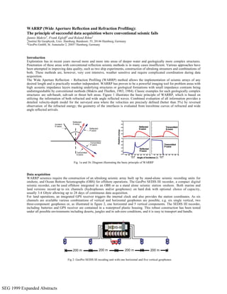
Fig. 1a and 1b: Diagram illustrating the basic principle of WARRP
h v vv v
200 m 200 m 200 m 200 m
v
SEDIS-III
Fig 2: GeoPro SEDIS III recoding unit with one horizontal and five vertical geophones
WARRP (Wide Aperture Reflection and Refraction Profiling):
The principle of successful data acquisition where conventional seismic fails
Jannis Makris1, Frank Egloff2 and Roland Rihm2
1Institut für Geophysik, Univ. Hamburg, Bundesstr. 55, 20146 Hamburg, Germany
2GeoPro GmbH, St. Annenufer 2, 20457 Hamburg, Germany
Introduction
Exploration has in recent years moved more and more into areas of deeper water and geologically more complex structures.
Penetration of these areas with conventional reflection seismic methods is in many cases insufficient. Various approaches have
been attempted in improving data quality, such as two ship experiments, construction of ultralong streamers and combinations of
both. These methods are, however, very cost intensive, weather sensitive and require complicated coordination during data
acquisition.
The Wide Aperture Reflection Refraction Profiling (WARRP) method allows the implementation of seismic arrays of any
desired length and is practically weather independent. WARRP has proven to be a powerful imaging tool for problem areas with
high acoustic impedance layers masking underlying structures or geological formations with small impedance contrasts being
undistinguishable by conventional methods (Makris and Thießen, 1983; 1984). Classic examples for such geologically complex
structures are sub-basalt, sub-salt or thrust belt areas. Figure 1 illustrates the basic principle of WARRP, which is based on
utilizing the information of both refracted and wide angle reflected waves. Combined evaluation of all information provides a
detailed velocity-depth model for the surveyed area where the velocities are precisely defined (better than 5%) by reversed
observation of the refracted energy; the geometry of the interfaces is evaluated from traveltime curves of refracted and wide
angle reflected arrivals.
Data acquisition
For land operations, an integrated GPS receiver triggers the internal clock and also provides the station coordinates. As six
channels are available various combinations of vertical and horizontal geophones are possible, e.g. six single vertical, two
three-component geophones or, as illustrated in figure 2, one horizontal and 5 vertical components. The SEDIS III recorder,
including batteries and GPS receiver are contained in a waterproof plastic housing. This robust construction has been tested
under all possible environments including deserts, jungles and in sub-zero conditions, and it is easy to transport and handle.
WARRP seismics require the construction of an ultralong seismic array built up by stand-alone seismic recording units for
onshore, and Ocean Bottom Seismographs (OBS) for offshore operations. The GeoPro SEDIS III recorder, a compact digital
seismic recorder, can be used offshore integrated in an OBS or as a stand alone seismic station onshore. Both marine and
land versions record up to six channels (hydrophones and/or geophones) on hard disk with optional choice of capacity,
usually 3.4 Gbyte allowing up to 28 days of continuous data acquisition.
-
SEG 1999 Expanded Abstracts

2. Fig 3: GeoPro SEDIS III Ocean
Bottom Seismograph
Fig. 4: Principle of offshore WARRP spread with schematic raypaths of
seismic energy propagation
seismic charge (5 kg to 20 kg) Distance [km]
32 54
30SEDIS #1 10 20
0 1SEDIS-III recording unit
Fig. 5: Schematic segment of an onshore WARRP spread. Each recording unit is equipped with 1 horizontal
geophone and 5 vertical geophones at 100m spacing. Shot size depends on section length.
Makris et al: WARRP - Wide Aperture Data Acquisition 2
For offshore application, the SEDIS III recorder is integrated in an OBS cased in a glass
sphere which can be deployed in water depths of up to 6000 m (see figure 3). The seismic
signals are recorded directly on the seafloor using gimble mounted geophones and/or
deep sea hydrophones. The instrument has no connection to the sea surface and is
retrieved by acoustic or time release.
Sensors are densely spaced, providing high resolution traveltimes, while the spreads are
long enough to ensure recording of wide angle reflections and diving waves for the
required depths. Array lengths range from 10 km to 100 km. Accordingly, the number of
seismic traces adds up to several hundreds for onshore operations while for offshore
surveys up to 100 six-channel OBS can be deployed. Seismic velocities can thus be
determined to the required depths continuously and with high resolution while first order
discontinuities are simultaneously sampled by wide angle reflections.
Offshore WARRP spread
The principle of an offshore WARRP spread is shown
in figure 4. A typical spread as stated above comprises
some 100 OBS, usually distributed at 500 m spacing.
After deployingthe OBS on the seafloor, the seismic
vessel sails over the OBS spread firing at 50 m
spacinga towed airgun array of vaiable capacity e.g. 8
guns or more with several thousand cu.in. volume. The
shots are recorded simultaneously by all OBS sensors
on the line. In order to locate the exact OBS position
on the seabed, one parallel line is shot at 1000 m
offsets to each line. In the final pass, the OBS are
acoustically released and, after surfacing are located
by radio and flash light, and retrieved. Navigation and
positioning is obtained by Differential Global Position
System (DGPS), which provides an accuracy of 5 m or
better as required.
Onshore WARRP spread
An example of a typical onshore WARRP spread is shown in figure 5. With 100 SEDIS-III landstations distributed at 500 m
spacing each recording 5 vertical and one horizontal geophones (i.e. receiver spacing of 100 m), a maximum offset of the
recording array of 50 km is obtained. Shotpoints are usually distributed at 300 m to 1 km intervals thus producing traveltime
sections that densely cover the geological section.
SEG 1999 Expanded Abstracts

3. NW SE
Distance (km)
0.0
0.2
0.4
0.6
0.8
1.0
1.2
1.4
24.0 25.0 26.0 27.0 28.0 29.0 30.0 31.0
TimeDistance/4.00(sec)
NW SE
Distance (km)
0.0
0.2
0.4
0.6
0.8
1.0
1.2
1.4
24.0 25.0 26.0 27.0 28.0 29.0
TimeDistance/4.00(sec)
Figs. 6a and 6b: (a) observed data of an OBS gather (b) computed data (finite differences) for the same OBS
Makris et al: WARRP - Wide Aperture Data Acquisition 3
Data processing
Magneto optical disks are used by the GeoPro SEDIS-III system to store seismic data recorded on hard disk in the field. These
are then processed on a UNIX based PC and Sun local area network (LAN). In addition to the seismic data, the following
information is also stored: acquisition parameters: (sampling rate, number of recording channels), date and time of initial clock
synchronization with an external GPS clock and final time comparison between the SEDIS internal clock and the external GPS
clock. Processing of the field data consists of demultiplexing, resampling to CWP/SU format and writing to SEG-Y tapes for
further data processing and modelling. As the internal clock of each recorder is subject to a temperature dependent drift, the
extracted data windows are time shifted in relation to UTC time according to the determined drift corrections.
The true location of every OBS on the seabed is obtained by the following procedure: 1) picking of first-arrival traveltimes from
observed sound propagating through the water, 2) transformation of geographical coordinates of shots and OBS into the local
coordinate system, 3) calculation of corrected OBS positions in the local coordinate system (rotation and translation) and 4)
transformation of final OBS positions back to geographical coordinates.
Velocity depth modeling
In order to interpret P- and S or converted waves the records are viewed and displayed for different offsets, with different scaling
and reduction velocities so that the modeling parameters can be optimised. Furthermore, general geological information is
utilised, if available. The seismic model is then obtained by tomographic inversion followed by forward modeling using an
optimised two-point ray-tracing package, based on the V. Cerveney and J.Psencik (1984) method. This process leads to a well
constrained velocity-depth model, in which first order discontinuities are constrained by reflected, and velocities by diving or
refracted waves. An initial estimate of the velocity structure is first established by a semi-automatic picking program. For the
first inversion, the initial model is optimised by a least square procedure from which a velocity model is obtained. This is
finalised when the observed traveltimes agree with those computed within the resolution of the observations. In order to improve
the derived velocity structure by the first break evaluation and define the limits of the geological formations, the velocity
gradients are substituted by first order discontinuities. Non linear inversion finalises the velocity structure. This is repeated from
top to bottom for each layer of the sequence. In each inversion of this iterative process, all events from each layer are considered.
The final model is now tested by forward modeling using the Ceveney-Psencik algorithm. The models have to satisfy the
kinematic and dynamic parameters of the sections, the amplitudes being calculated by the Joerppitz equations. Finally, synthetic
sections can be computed by the finite difference method.
Accuracy
Resolution and reliability of the WARRP method depend not only on the Fresnel Zones, which are functions of the frequency of
the primary seismic pulse and the velocity structure at depth, but also depend on the spacing of the shots and geophones. The
great data redundancy, where the velocity model is controlled by a multitude of data, permits the development of a consistent
and strongly constrained velocity-depth model. The use of different reduction velocities and data displays helps to identify
features that otherwise might remain undetected. It is estimated that the velocity determination in the upper layers to approx. 2
km depth is better than 0.1 km/s. Since the error is cumulative with increasing depth, in the lower part of the model, the accuracy
of the velocity determination deteriorates. It has been estimated to be within ± 5%. Errors in the depth of a reflecting interface of
50 m or more would also lead to a significant mismatch between observed and calculated traveltimes and is usually detectable.
Dynamic modeling
In order to check the validity of an obtained velocity-depth model, dynamic modeling is performed by calculating synthetic
seismogram sections. Comparison of synthetic with recorded seismic signals allows a more direct comparison by visualisation
SEG 1999 Expanded Abstracts

4. NW SE
Distance (km)
0.0
1.0
2.0
13.0 12.0 11.0 10.0 9.0 8.0 7.0 6.0 5.0 4.0 3.0 2.0 1.0 0.0
(C) WARPSEC, Version 2.6
TimeDistance/4.00(sec)
Fig. 7a and 7b: (a) shot gather of OBS section, (b) migrated image of red framed area of OBS section on left side
Makris et al: WARRP - Wide Aperture Data Acquisition 4
of the recorded seismic energy leading to a better understanding of the nature of the recorded signals. Examples are presented in
figures 6a and 6b.
The program used to compute the synthetic seismic wavefield solves the acoustic wave equation by finite-differences (Pilipenko,
1979, 1983). The velocity-depth model used for the wavefield calculations is taken from the results obtained from the ray-tracing
modeling (Cerveny and Psencik, 1984). The synthetic data are presented in Seismic Unix (SU) format (Cohan and Stockwell,
1998).
WARRP migration
Since ray-tracing tends to smooth the mapped discontinuities, a special WARRP migration technique was developed by
Pilipenko and Makris, 1997 that helps to overcome this problem. The algorithm is applicable to refracted and diving waves but
not to reflected waves and transforms the observed time-fields at depth for every identifiable event. Each shot gather is migrated
separately and then all depth-migrated elements of a given discontinuity are superimposed to produce the accurate geometry. In
this way every seismic layer can be reconstructed over the complete seismic section allowing the identification of faults and
small structural displacements that ray-tracing would have left undetected. Figures 7a and 7b show one shot gather section (out
of 100 different positions available) of an offshore profile and the migrated image of that part of the section.
Conclusions
The WARRP technique as developed during the past few years evolved from an academic approach to a sophisticated,
competetive method of high standard. WARRP allows the penetration of deep reflectors even where the impedance contrast is
unfavourable. In particular offshore as well as onshore target areas in sub-salt, sub-basalt or thrust belt environments may be
resolved where normal incident methods fail. WARRP offers a great flexibility of survey design, e.g. in coastal areas, where on-
and offshore surveys can be combined with stations distributed in 2-D or 3-D grids, providing continuous and consistent data
across shorelines and in shallow water areas.
In addition, the WARRP technique is economic and time effective in large scale reconnaissance surveys especially in areas of
difficult access . It can be combined with normal incidence seismics to produce a complete seismic image of the subsurface.
References
Cerveny and Psencik, 1984, SEIS83 - Numerical modeling of seismic wave fields in 2-D laterally varying layered structures by the ray method.
Cohen and Stockwell, 1998, CWP/SU : Seismic Unix Release 32 : a free package for seismic research and processing. Center for Wave Phenomene, C. S. of Mines.
Makris, J. and Thießen, J. 1983, Offshore seismic investigations with a newly developed ocean bottom seismograph, 53rd ann. SEG meeting, Las Vegas
Makris, J. and Thießen, J., 1984, Further development and test of a new measuring system for offshore refraction seismics and hydrocarbon exploration, 54th.SEG
Meeting, Atlanta
Makris, J., 1995, Wide Angle Reflection Profiling - Applications for Petroleum Exploration and Crustal Studies. 11th ASEG conference, Adelaide, Australia
Pilipenko, V.N., 1979, Numerical method of time field for seismic boundary construction. Inverse kinematic problems of explosion seismology, Moscow (in Russian)
Pilipenko, V.N., 1983, Continuation of the wave field using the finite-difference solution of the wave equation. Application of numerical methods to the researches of
the Lithosphere, Novosibirsk (in Russian)
Pilipenko and Makris, 1997, Application of migration to the interpretation of WARP data. Expanded Abstract of the 69th SEG Meeting, Dallas
SEG 1999 Expanded Abstracts