Downloaded 350 times


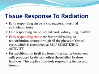

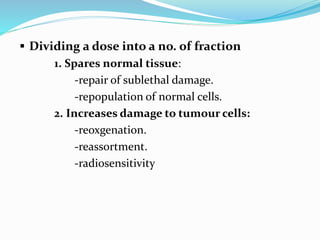
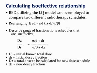
![EXAMPLE : Let us suppose we are giving 40Gy/16# for a tumour
@ 2.5Gy/#. But we want to give4Gy/#.
i.e. D1 = 40 Gy, d1 = 2.5 Gy, d2 = 4 Gy
D2/D1 = d1+ (α /β ) / d2 + (α /β)
D2=40 [2.5 + 10/4 +10 ]
D2=40[12.5/14]
D2=35.72Gy
So we have to give 35.72 Gy in 9 #.](https://image.slidesharecdn.com/h7mbmbgmqs2rgubihipn-signature-eaf12d6eca54dc17cb0f861df5438b7d6558073f64c8818c45af2f13932cdafa-poli-180401072641/85/Linear-quadratic-model-ppt-45-320.jpg)


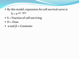
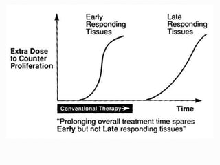
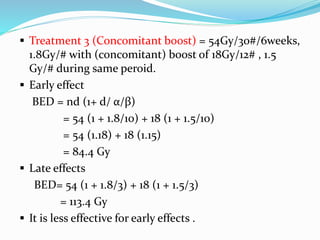
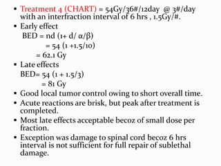
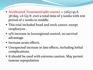
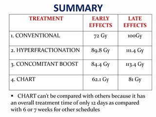
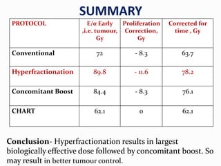
This document summarizes key concepts regarding radiation-induced cell death and survival curves. It discusses how cell death is defined for differentiated and proliferating cells. The linear-quadratic model is then explained, which describes cell survival curves using alpha and beta coefficients. Various fractionation schemes and their resulting biological effective doses are calculated and compared for treating different head and neck cancers. The limitations of hypofractionation and importance of accounting for tumor proliferation are also covered.


![Arc therapy [autosaved] [autosaved]](https://cdn.slidesharecdn.com/ss_thumbnails/arctherapyautosavedautosaved-150423125828-conversion-gate01-thumbnail.jpg?width=640&height=640&fit=bounds)


![Chapter 39 role of radiotherapy in benign diseases.pptx [read only]](https://cdn.slidesharecdn.com/ss_thumbnails/chapter39roleofradiotherapyinbenigndiseases-191105205437-thumbnail.jpg?width=640&height=640&fit=bounds)


