
Recommended
Recommended
More Related Content
Similar to Review Journal 1A simplified mathematical-computational model of .docx
Similar to Review Journal 1A simplified mathematical-computational model of .docx (20)
More from michael591
More from michael591 (20)
Recently uploaded
Recently uploaded (20)
Review Journal 1A simplified mathematical-computational model of .docx
- 1. Review Journal 1 A simplified mathematical-computational model of the immune response to the yellow fever vaccine 1. This model can be improved in a way if there are more test subjects and more variables and parameters with test data is added. Plus the mathematical process is always improvable so if there is an equation which is more better for this experiments then it’s can improve the model and experiment with development. Another try is to improve the qualitative results obtained from our model. Additional computational experiments, such as the effects of a) a booster dose and b) a reduction in the population of TCD8+ naive. Also, a sensitivity analysis will be performed to identify sensitive parameters and to identify connections between change in parameters values and computational results. 2. if more cases or more experiments were added then it could be more expanded research and could improve the research more but the similar results are achieved by the shorter experiments so we can say this number of experiments were enough. But there is always a room left for improvements. The second difference between the two models is that this work reduces the amount of equations from 19 to 10. The reduced model described in this work considers only the main populations of cells and molecules involved in the response to the vaccine, and abstracts some details that are not crucial to represent the behavior of the immune response. For example, the distinct compartments are not represented here. Also, some populations were not considered because no experimental data is available to validate the simulations, such as the CD4+ T cells. In future, more cell or molecule can be included in the model again, if its role is important to explain or represent some behavior that the reduced model presented in this section could not represent. That was something in the first paper journal which was not satisfactory for me.
- 2. 3. This model can be applied to the numerous medical applications like cancer immunity and other immune vaccinations for the diseases or viruses in the open environment which are lethal and are possible to cure in the future. The virus cannot proliferate itself, it needs to infect a cell and use it as a factory for new viruses. This is implicitly considered in the term πvV , which represents the multiplication of the virus in the body, with a production rate πv. The term cv1V cv2+V denotes a non-specific viral clearance made by the innate immune system 4. The main problem which was to solve is that the author needs something authentic calculations to perform the experiment to show the results of that experiment as negative and for that only programming and developing an algorithm or a program is not enough. It needs the proper calculations of the human body and cells about each and every details in depth. So that’s why it was necessary to include the calculations in the immune system development. Previously the author wasn’t including proper calculations so the API for python wasn’t providing the accurate results. Because the default made up API’s would response only to limited calculations. But he need some extensive and complex calculations so it was necessary to include it in. in this research mathematical model is being used as a tool to assist the research in vaccinology and public health. With the use of mathematical and computational models, it is possible to experiment, in silico, different scenarios related to vaccination, for answering important questions still open. 5. The model discussed in this paper is based on the previous study on mathematical model which describes the human immune response to the infection by YF virus. For this development of the model code was built in python programming which included libraries for solving mathematical problems. It was scipy. It was tested on different human cells and each of the antibody response generates the results of the experiments and test. The model is then evaluated using distinct scenarios, and as will be shown, it was able to qualitatively
- 3. reproduce some experimental results reported in the literature. The results were found to be improved than in the previous study and the conclusion for the paper is that he validated the model with two distinct scenarios that were simulated. The first one simulates the immune response to the administration of the standard dose of the 17DD-YFV. The second one simulates the immune response to distinct doses of vaccine and then compared the two results to find out the best. References Bonin, C., Fernandes, G., dos Santos, R., & Lobosco , M. (2017). A simplified mathematical-computational model of the immune response to the yellow fever vaccine. 7-8. Kumar, M., A. S., MB, M. M., Vinodini , V. M., & Lakshmi , A. K. (2018). Forecasting of Annual Crime Rate in India : A case Study . International Conference on Advances in Computing, Communications and Informatics, 6. Forecasting of Annual Crime Rate in India Case study analysis ( June 7 , 2019 ) Question 1 In this the authors are finding ways to manipulate the best thing and equations which will help them to precisely measure the strategic procedures regarding criminality rate and controlling the uprising rate of crime. The equations are the best thing to describe the proceeding and calculating the rate of crime which has to lessen at any cost.
- 4. After the brief and intellectual description of the equation authors have ways to mend them along with the care and prevention of the people’s behavior and environmental related factors. · ARIMA which autoregressive integrated moving average is the good and expressive equation built up of the steps towards the mortality rate of crime. · The forecasting of the crime has made easy for the authors and police departments by manipulating the findings of a case. · Orders of crime in this have been described by China research and the early findings of a planning. Analyses of the model and socially interlinking of crime in plotting the analyses and data structures of the person’s social behavior which affect the homicide and unemployment victims. This data has now been computerized and elevated in the database of our system. The Box-Jenkins model proved to be the best model with the precise and data analyses testing the best essential series of criminal cases. Question 2 The model Box-Jenkins has the most precise and analytical way to evaluate the best and improving tribe to control and prevent crime technologies. The building of the urban areas has the greater values towards the dynamic pursue of the technology base crime basis. Collection of the historic data from the previous eras is the major hindrance in fluctuating environments, the crime rate through the social interlinking and touching the boundaries of the extreme provision of exposure of a person personal data. · The parameters were the historical crime related data collection and seasonal theft varying communities produce a great impact on this collection of the data. · Non-stationary peak of crime rate may have an affecting way to kill the possibilities and hope in finding the exact location of the crime server. The model was built on the basis and practical supervision depending on the areas and police departments allocating in that
- 5. area. Question 3 The model was tested based on the collected data. Providing one of the control group which has the recent studies of the crime rate and the other have the possible growing hub of gangs interlinked in urban areas from the starting. By calculating through the equation precisely, and improving data and results stood up in front of the research team. · Hardships do come in doing such a risky job which is equal to, putting your hand in the mouth of an alligator and spectating the thing which is causing suffocation. Question 4 The results were good enough and helping towards what was expected by the authors, crime strategy has been broken through it and dismantle the connection networks indulging in crime. The model was built to measure the precise analyses intruding and indulging the different possibilities in enhancing the equation oriented crime analyses. · Sharing through the third parties series of cases have been detected to control and manage the outcomes, developing techniques will enhance the data accuracy and security. Question 5 Logical researching based on the right way to manipulate case studies and testing the hypothesis has a great impact on the rest of the experimental studies. Urban areas have the highest rate of crime, it’s all because the easy availability of data access and approach of persons from street to street so the security must be provided to the users. The advantage of the devices and social interconnection has been the major outcome of the crime related problems and being better to understand it will also mend ways towards more capturing of pre-planned crime on scenes. References 1. Kumar, M., S, A., & MB, M. M. (2018). Forecasting of Annual Crime Rate in India: A case Study. Center for Excellence in Data Engineering and Computational Modeling
- 6. Indian Institute of Information Technology and Management- Kerala. Forecasting of Annual Crime Rate in India:A case Study Manish Kumar, Athulya S, Mary Minu MB, Vidya Vinodini M D, Aiswaria Lakshmi K G, Anjana S, Manojkumar TK* Center for Excellence in Data Engineering and Computational Modeling Indian Institute of Information Technology and Management- Kerala (IIITM-K) Abstract— Crime forecasting has been made possible by criminological theories and developments in computational techniques/data analytics further improved the technologies of forecasting. It helps the various departments of the police to make a decision and strategy to prevent the crime. This paper focuses on forecasting the annual crime rate in India using the Time Series Models such as Auto-Regressive Integrated Moving Average (ARIMA) and Exponential Smoothing. Source of data is from the National Crime Record Bureau of India. As a part of modeling, data is divided into training data for the years 1953 to 2008 and test data for the years 2009 to 2013. By examining the model, it’s clear that the forecast values are within the 95% confidence interval of the test data and accuracy measurements are also significant. Hence the time series model suitable for crime forecasting.
- 7. Keywords—crime forecasting; ARIMA Model; Exponential Smoothing Model I. INTRODUCTION India is having high population growth rates compared with the rest of the world. India’s population is estimated to be around one billion. The high population density, combined with other factors such as lack of jobs, poverty, and illiteracy will result in a higher violence rate. The crime and violence rate vary from state to state. States like Uttar Pradesh, Bihar etc records high crime rates according to 2017 statistics. Like other counties increase in crime rate is a major concern in India also. From the reports of National Crime Record Bureau (NCRB), states that most of crime incidents recorded is in urban area [1]. In India, crime rate (case reported per lakh population) has increased from 166.7 to 215.5 in years from 1953 to 2013. By analyzing the data, crime rates got highly fluctuated in the years 1970-2005. The statistics indicate that crime rate in India is steadily increasing for the past 8-9 years. The increasing trends in urban crime lead to various other violations of law and make life harder. Crime forecasting will help in analyzing crime rates and one can take preventive steps for reducing the number of crimes. Time series is reported to be one of the best tools for analyzing time series data and providing proper insights into various dependent factors of the series. Since Autoregressive Integrated Moving Average (ARIMA) model was created by Box and Jenkins, it has been effectively utilized as a part of forecasting economic, marketing, production, social issues etc[2]. This model has the advantage of exact forecasting over short-term for the series. This paper used Box-Jenkins Methodology to model Annual Crime Rate Time Series (ACRTS) by using ARIMA models
- 8. and Exponential smoothing model [3]. The ARIMA model could provide forecasting results with upper limits, lower limits and forecasted values, which means any realization within the interval between upper limits and lower limits will be accepted. The efficient approach to identify and analyze patterns and trends in crime can be made by applying crime analysis and prevention. With the increasing advent of technologies in crime, data analysts may help the police officers to speed up the process of solving crimes. II. METHODS The review of the literature for this work outlines the papers that deals with the technique carried out for forecasting crime rates, their challenges and to take remedial actions on it etc. Utilizing time series model to make short-term forecasting of crime is a new research field appearing recently. Peng Chen et.al gave a proportional study for the forecasting crime using the ARIMA model, in this paper ARIMA is used to make short-term forecasting of property crime for one city of China. They used the ARIMA model for making short-term forecasting of property crime for one city of China, then compared forecasting results with the Simple Exponential Smoothing (SES) and Holt’s two-parameter exponential smoothing (HES). Noted that the ARIMA model has best fitting and forecasting accuracy than other two models [4]. Arye Rattner presents an attempt in social indicators and crime rate forecasting, to use macrodynamic social indicators in a time series analysis of three crime categories-homicide; property and; robbery offenses in Israel. By analyses, models are created for the earlier findings in the relationship between homicide and unemployment, and density of population and property offenses [5]. Shrivastav and Ekata validate the applicability of the
- 9. ARIMA model in crime forecasting. Here they utilized the crime data of Gujarat State pertaining to counterfeiting of currency. The authors focused to plot the matter-of-facts which need to be undertaken to use Box Jenkins ARIMA time series models [3]. N.Mohamad Noor proposed crime forecasting using Autoregressive Integrated Moving Average (ARIMA) model and fuzzy alpha-cut method. This combination is expected to generate more accurate forecasting result with a 978-1-5386-5314-2/18/$31.00 ©2018 IEEE 2087 minimum error. The results will help the authorities in making the right decision in crime prevention strategies [6]. Research based on crime forecasting has a prominent role in the forecasting world. Many forecasting methods have been applied in this field as Naïve lag, exponential smoothing, decomposition method and ARIMA model [7]. Using a time series model to predict the values for future reference is relatively rare in the world. The outcomes make an impact for the right decision in taking preventions against crime. The results could give data about crime trends particularly the conceivable most evidently bad and better condition afterward. This data can help the police in settling on choice for operational and strategic procedures in crime prevention. III. THEORETICAL FRAMEWORK A. Data Source and Software The data were collected from National Crime Bureau of India (www.ncrb.gov.in). Statistical tool R was used for time series modeling [1]. B. Box-Jenkins Model
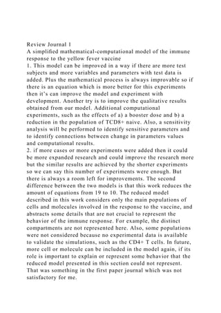
- 10. The basic idea of Box-Jenkins approach in modeling a time series is summarized in Fig 1. Box-Jenkins consists of three phases [8]. The following phases are • Identification: Selects the best model based on analysis of series. • Testing and Estimation: In this stage the parameters are estimated and they are used for forecasting and then residuals are evaluated. Then these residuals are examined for validation of mode. If following conditions are satisfied, we may proceed further for forecasting using that particular data set. a. These residuals should be stationary. b. The residuals should have zero autocorrelation coefficients between them. c. It is expected that these residuals are normally distributed. If all these are satisfied, use that mode for forecasting out of sample. Otherwise go to first phase and select another mode. Fig. 1. Box Jenkins Methodology C. Exponential Smoothing
- 11. This method is based on the principle that recent values have more weight and it decreases as the observation gets older. There is a variety of exponential methods but all they have in common is recent values are given relatively more weight than older observations [9]. 1) Single Exponential Smoothing In Single Exponential Smoothing, forecasting is done using previous period forecast value and adjusts it using forecasting error. = + ( − ) (1) value lies between 0 and 1 So the equation involves a basic principle of negative feedback. The past forecast error is used to correct the next forecast. An alternative way of writing equation is = + (1 − ) (2) On solving, we get = + (1 − )[ + (1 − ) ] = + (1 − ) + (1 − ) Here it is clear that has less weightage than and weightage is decreasing exponentially. But if there is trend in the series, the forecast will lag behind the trend because there is no parameter which can be used to match trend. 2) Holt Linear Method
- 12. Holt Linear Method, which is an extension of Single Exponential Smoothing that allows to forecast data with trend given by Holt in 1957 [10]. Holts linear exponential smoothing using two parameters and . = + (1 − )( + ) (3) = ( − ) + (1 − ) (4) = + (5) denotes the estimate of level time t, denotes the estimate of trend at time t. Equation (3) adjust level at time ( ) directly for trend of previous period and adding it to last smoothed value . This helps to estimate the trend and bring the level to approximate level of current data. Equation (4) update the trend on the difference between last smoothed value and it is appropriate because it will show the trend in previous and some randomness can be smoothed by using . This is similar to Single Exponential Smoothing but used for updating the trend. Equation (5) is used to forecast for future values. This method is sometimes called Double Exponential Method [11]. This method is very good for the data that have trend and very 2088 useful but they will lack for modeling the time series when
- 13. there will be seasonality with trend. 3) Holt Winters Method This method occurs when seasonality comes into effect. Holt’s method was extended by Winters to capture seasonality directly. In fact, there are two types of seasonality additive or multiplicative [12]. So we have two types of Holt Winters method for seasonality as follows :- a) Multiplicative Seasonality = ⁄ + (1 − )( + ) (6) = ( − ) + (1 − ) (7) = ⁄ + (1 − ) (8) = ( +) ( ) b) Additive Seasonality = ( − ) + (1 − )( + ) (10) = ( − ) + (1 − ) (11) =
- 14. ( − ) + (1 − ) (12) = + + (13) Where, denotes level at time t denotes trend denotes seasonality denotes forecasted values D. ARIMA MODEL Auto Regression Integrated Moving Average(ARIMA) model has been studied extensively. They were popularized by George Box and Gwilym Jenkins in early 1970s. The ARIMA model is the most general class of model for forecasting a time series like other method[13]. It requires only historic time series data. Normally the ARIMA model is denoted by the ARIMA (p, d, q) p is number of autoregressive term d is number of non-seasonal difference q is number of lagged forecast error Now if d=0, then ARMA (p, q) is known as stationary model that is it can be used for only stationary series. While in ARIMA if d > 0 that is non-stationary model. If underlying time series is nonstationary, then difference method is used to make it stationary. The order of difference determines the value of I. I (0) means original time series is stationary. I (1) means first order differenced series is stationary. The equation for ARIMA model is given as
- 15. (1 − θ B)(1 − B)Y = c + (1 − θ B)E (14) And after differencing the series ARMA is applied on the time series. In ARIMA model, AR (Auto Regressive) component represent the memory of process for preceding observation. So p represents the auto regressive component in ARIMA (p, d, q). If other components are zero then it is represented by AR (p) and equation is given by Y = c + ∅ Y +⋯⋯⋯⋯+ ∅ Y + E (15) Where ∅ represent the magnitude of relationship. If p is 0 then it means that there is no relationship between adjacent terms. The lag of forecast error is called Moving Average. These represent the memory for random shock. q represent the number of moving average component. Then it is represented by MA (q) and equation is given by Y = c + E − θ E − θ −⋯⋯⋯⋯θ E (16) Where θ, represents the magnitude of relationship. IV. MODELING ACRTS In this section, the Annual Crime Rate Time Series (ACRTS) has been modeled by using Time Series models. ARIMA model and exponential smoothing method is used to model the CRTS. A. ARIMA Modeling The Box – Jenkins Methodology is used to build a model.
- 16. In Box-Jenkins Methodology there are three steps which were followed to built ARIMA model and Exponential Smoothing for CRTS 1) Data analysis and Test for stationary-ACRTS Fig.2 represents the Time Series plot of training data of ACRTS. It is clear from the plot that the series is non- stationary. We confirmed the non-stationary by calculating Augmented Dickey-Fuller(ADF).. The ADF test performed on data shows the p-value 0.5413 which strongly suggests that the series is non-stationary i.e. the mean is not constant. To make data stationary first order difference is performed and hence the series became stationary. Fig.3 shows the first order differenced time series of the annual crime rate. Fig. 2. ARCTS for Training Data 2089 Fig. 3. ACR First Order Differenced Time Series.
- 17. The ACF and PACF plots are used to identify the models. Fig.4 and Fig.5 are the plots of ACF and PACF of differenced series. The order of difference to make series stationary is 1 it implies the model will be ARIMA (p, 1, q). On basis of the correlogram of ACF and PACF the value of p and q are chosen. By considering several models as shown in TABLE 1, the model which produce minimum AIC and BIC is chosen. Hence the model ARIMA (0, 1, 0) with minimum BIC and model ARIMA (2, 1, 2) with minimum AIC were taken for analysis. While comparing the residuals and accuracy the best fit model to forecast ACRTS is ARIMA (2, 1 ,2). Fig. 4. ACF of ACR Differenced Time Series Fig. 5. PACF Plot of ACR Differenced Time Series TABLE I. COMPARISON OF ARIMA MODELS 2) Testing and Diagnostics Testing is the second phase of the Box-Jenkins
- 18. Methodology. In this phase after fitting the model, the residuals are tested for verification of model fitting. The residual should follow these tests. • There should be no correlation between the residuals i.e. residual should be independent of each other. • The residual should follow white noise. • The residual should be normally distributed. Fig.6 shows the plot of ACF of residuals and it is clear that there is no spike in this plot which means there is no correlation between the residuals [14]. For residuals to be white noise model the Box –Ljung test is applied on the residuals. The null hypothesis for this test is that the series follows a white noise model and p-value for the Box-Ljung test was obtained suggesting that it accept the null hypothesis which means residuals follow the white noise models. To check the normality of residuals there is the test called Jarque-Bera test. In this test null hypothesis in the series follows the normal distribution. The p-value obtained is high suggesting that to accept the null hypothesis means residuals are normally distributed [15]. So by testing the residuals, it concluded that ARIMA (212) can be used for forecasting. Fig. 6. ACF of Residual 3) Forecasting
- 19. After verifying and testing it is clear that the ARIMA (212) can be used for forecasting the test data (2008-2013). All observed test data lie between the 95% confidence interval forecasted by the ARIMA (212). Fig.7 shows the actual and forecasted value by ARIMA (212) Fig. 7. Forecasted value vs actual value ARIMA MODEL AIC BIC 010 399.68 401.69 110 401.38 405.39 111 402.27 408.29 112 398.73 406.76 211 396.93 404.96 212 394.76 404.79 2090
- 20. 4) Accuracy Accuracy refers to “goodness of fit”, which in turn refers how well the forecasting model is able to reproduce data that are already known [16]. There are many standard statistical measures used for measurement of accuracy. • MAE-Mean Absolute Error (the mean value of absolute errors) • MASE-Mean Absolute Squared Error (the mean value of errors square) • MAPE-Mean Absolute Percentage Error. So the best model have low values for these measurements. The measurements for ARIMA(212) are given below in Table II TABLE II. ACCURACY MEASUREMENT FOR ARIMA (212) MODEL Data Set MAE MAPE MASE Training Set 5.92 3.43 0.86 Test Set 12.93 6.33 1.88 B. Exponential Smoothing Modeling To model ACRTS using exponential smoothing model, the following steps were used. 1) Data analysis and Model selection
- 21. By analyzing the trend of ACRTS in Fig 2, it is quite difficult to summarize, as its trend shows both increasing and decreasing[14]. Thus to make result more accurate Holt Linear method is introduced which is an extension of single exponential smoothing. Thus the Holt Linear method provided the best fit for ACRTS. 2) Initialization and Estimation of parameter Initialization of Holt Winters function is made using R with the value of gamma equal to false (means there is no gamma in Holt linear Model) and the optimal value of coefficient α and β is given as is α = 0.943 β = 0.181 These values indicate the dependence of value on previous data. Fig 8 shows the fitted value of data by Holt linear model. It is clear that fitted values are following pattern of observed values.
- 22. Fig. 8. Holt linear modelling vs Train data 3) Testing and Diagnostics ACF plot for residuals of Holt linear model is shown in Fig.9 .It is clear that there is no autocorrelation between the residuals. Fig. 9. ACF residual of Holt linear Model Hence Holt Linear models can be used as a best fit model for forecasting the ACRTS (2008-2013). Fig 10 shows the forecasted value vs. test data. All observed test data lie between the 95% confidence interval forecasted by the Holt Linear. Fig. 10. Forecasted value vs Test Data 4) Accuracy Accuracy measurements of Holt Linear methods are given below in Table III. The values of measurements are significant. It concludes that Holt Linear method is numerically significant for modeling ACRTS. TABLE III. MEASUREMENT FOR HOLT LINEAR MODEL
- 23. Data Set MAE MAPE MASE Training Set 7.48 4.36 1.09 Test Set 9.23 4.50 1.34 2091 V. RESULT The Annual Crime Rate in India for the years 2014-2018 are evaluated by Holt Linear Method is shown in Table IV. TABLE IV. FORECASTED VALUE BY HOLT LINEAR METHOD Year Point Forecast Lo80 Hi80 Lo95 Hi95 2014 161.2 153.4 202.5 98.1
- 26. 261.1 Table V contains the value forecasted by ARIMA (212) TABLE V. FORECASTED VALUE BY ARIMA (2 1 1) Year Point Forecast Lo80 Hi80 Lo95 Hi95 2014 190.8 146.8 234.8 123.5 258.1 2015 192.4 141.8
- 28. 260.4 96.7 294.6 2018 197.3 125.3 269.3 87.1 307.4 VI. CONCLUSION AND FUTURE WORK This paper concluded that time series model can be applied for crime forecasting. The result obtained from both the models conclude that they are significant for forecasting all test data which are lying between a 95% confidence interval and accuracy measurements for training data shows that they are numerically significant. In future, we are trying to analyze
- 29. crime against women, children so that we can predict how much police strength is convenient to decrease the crime rate. VII. REFERENCE [1] Official webportal of National Crime Records Bureau http://ncrb.gov.in/ [2] Box, George EP, and David A. Pierce. "Distribution of residual autocorrelations in autoregressive-integrated moving average time series models." Journal of the American statistical Association 65.332 (1970): 1509-1526. [3] Shrivastav, Anand Kumar. "Applicability of Box Jenkins ARIMA model in crime forecasting: A case study of counterfeiting in Gujarat state." International Journal of Advanced Research in Computer Engineering & Technology (IJARCET) 1.4 (2012): pp-494. [4] Chen, Peng, Hongyong Yuan, and Xueming Shu. "Forecasting crime using the arima model." Fuzzy Systems and Knowledge Discovery, 2008. FSKD'08. Fifth International Conference on. Vol. 5. IEEE, 2008 [5] Rattner, Arye. "Social indicators and crime rate forecasting." Social Indicators Research 22.1 (1990): 83-95
- 30. [6] Noor, Noor Maizura Mohamad, et al. "Crime forecasting using ARIMA model and fuzzy alpha-cut." Journal of Applied Sciences 13.1 (2013): 167-172 [7] Groff, Elizabeth R., and Nancy G. La Vigne. "Forecasting the future of predictive crime mapping." Crime Prevention Studies 13 (2002): 29-58. [8] Loftin, Colin, and David McDowall. "The police, crime, and economic theory: An assessment." American Sociological Review (1982): 393-401. [9] Williams, Billy, Priya Durvasula, and Donald Brown. "Urban freeway traffic flow prediction: application of seasonal autoregressive integrated moving average and exponential smoothing models." Transportation Research Record: Journal of the Transportation Research Board 1644 (1998): 132-141. [10] Gorr, Wilpen, Andreas Olligschlaeger, and Yvonne Thompson. "Short- term forecasting of crime." International Journal of Forecasting 19.4 (2003): 579-594 [11] Flaxman, Seth R. A General Approach to Prediction and Forecasting Crime Rates with Gaussian Processes. Heinz College Technical
- 31. Report, 2014. URL https://www. ml. cmu. edu/research/dap- papers/dap_flaxman. pdf, 2014 [12] Gorr, Wilpen, Andreas Olligschlaeger, and Yvonne Thompson. "Assessment of crime forecasting accuracy for deployment of police." International Journal of Forecasting (2000): 743-754 [13] Alwee, Razana, et al. "Hybrid support vector regression and autoregressive integrated moving average models improved by particle swarm optimization for property crime rates forecasting with economic indicators." The Scientific World Journal 2013 (2013) [14] Mutangi, Kudakwashe. "Time Series Analysis of Road Traffic Accidents in Zimbabwe." International Journal of Statistics and Applications 5.4 (2015): 141-149. [15] Ott, R. Lyman, and Micheal T. Longnecker. An introduction to statistical methods and data analysis. Nelson Education, 2015 [16] McClusky, Howard Y. "An Introduction to Statistical Method." (1925): 549-551 2092 <<
- 32. /ASCII85EncodePages false /AllowTransparency false /AutoPositionEPSFiles true /AutoRotatePages /None /Binding /Left /CalGrayProfile (Gray Gamma 2.2) /CalRGBProfile (sRGB IEC61966-2.1) /CalCMYKProfile (U.S. Web Coated 050SWOP051 v2) /sRGBProfile (sRGB IEC61966-2.1) /CannotEmbedFontPolicy /Error /CompatibilityLevel 1.7 /CompressObjects /Off /CompressPages true /ConvertImagesToIndexed true /PassThroughJPEGImages true /CreateJobTicket false /DefaultRenderingIntent /Default /DetectBlends true /DetectCurves 0.0000 /ColorConversionStrategy /LeaveColorUnchanged /DoThumbnails false /EmbedAllFonts true /EmbedOpenType false /ParseICCProfilesInComments true /EmbedJobOptions true /DSCReportingLevel 0 /EmitDSCWarnings false /EndPage -1 /ImageMemory 1048576 /LockDistillerParams true /MaxSubsetPct 100 /Optimize true /OPM 0 /ParseDSCComments false /ParseDSCCommentsForDocInfo true /PreserveCopyPage true
- 33. /PreserveDICMYKValues true /PreserveEPSInfo false /PreserveFlatness true /PreserveHalftoneInfo true /PreserveOPIComments false /PreserveOverprintSettings true /StartPage 1 /SubsetFonts true /TransferFunctionInfo /Remove /UCRandBGInfo /Preserve /UsePrologue false /ColorSettingsFile () /AlwaysEmbed [ true /AbadiMT-CondensedLight /ACaslon-Italic /ACaslon-Regular /ACaslon-Semibold /ACaslon-SemiboldItalic /AdobeArabic-Bold /AdobeArabic-BoldItalic /AdobeArabic-Italic /AdobeArabic-Regular /AdobeHebrew-Bold /AdobeHebrew-BoldItalic /AdobeHebrew-Italic /AdobeHebrew-Regular /AdobeHeitiStd-Regular /AdobeMingStd-Light /AdobeMyungjoStd-Medium /AdobePiStd /AdobeSongStd-Light /AdobeThai-Bold /AdobeThai-BoldItalic /AdobeThai-Italic /AdobeThai-Regular /AGaramond-Bold
- 66. /ZapfChancery-MediumItalic /ZapfDingbats /ZapfHumanist601BT-Bold /ZapfHumanist601BT-BoldItalic /ZapfHumanist601BT-Demi /ZapfHumanist601BT-DemiItalic /ZapfHumanist601BT-Italic /ZapfHumanist601BT-Roman /ZWAdobeF ] /NeverEmbed [ true ] /AntiAliasColorImages false /CropColorImages true /ColorImageMinResolution 150 /ColorImageMinResolutionPolicy /OK /DownsampleColorImages true /ColorImageDownsampleType /Bicubic /ColorImageResolution 300 /ColorImageDepth -1 /ColorImageMinDownsampleDepth 1 /ColorImageDownsampleThreshold 2.00333 /EncodeColorImages true /ColorImageFilter /DCTEncode /AutoFilterColorImages true /ColorImageAutoFilterStrategy /JPEG /ColorACSImageDict << /QFactor 0.76 /HSamples [2 1 1 2] /VSamples [2 1 1 2] >> /ColorImageDict << /QFactor 0.76 /HSamples [2 1 1 2] /VSamples [2 1 1 2] >> /JPEG2000ColorACSImageDict << /TileWidth 256
- 67. /TileHeight 256 /Quality 15 >> /JPEG2000ColorImageDict << /TileWidth 256 /TileHeight 256 /Quality 15 >> /AntiAliasGrayImages false /CropGrayImages true /GrayImageMinResolution 150 /GrayImageMinResolutionPolicy /OK /DownsampleGrayImages true /GrayImageDownsampleType /Bicubic /GrayImageResolution 300 /GrayImageDepth -1 /GrayImageMinDownsampleDepth 2 /GrayImageDownsampleThreshold 2.00333 /EncodeGrayImages true /GrayImageFilter /DCTEncode /AutoFilterGrayImages true /GrayImageAutoFilterStrategy /JPEG /GrayACSImageDict << /QFactor 0.76 /HSamples [2 1 1 2] /VSamples [2 1 1 2] >> /GrayImageDict << /QFactor 0.76 /HSamples [2 1 1 2] /VSamples [2 1 1 2] >> /JPEG2000GrayACSImageDict << /TileWidth 256 /TileHeight 256 /Quality 15 >> /JPEG2000GrayImageDict <<
- 68. /TileWidth 256 /TileHeight 256 /Quality 15 >> /AntiAliasMonoImages false /CropMonoImages true /MonoImageMinResolution 1200 /MonoImageMinResolutionPolicy /OK /DownsampleMonoImages true /MonoImageDownsampleType /Bicubic /MonoImageResolution 600 /MonoImageDepth -1 /MonoImageDownsampleThreshold 1.00167 /EncodeMonoImages true /MonoImageFilter /CCITTFaxEncode /MonoImageDict << /K -1 >> /AllowPSXObjects false /CheckCompliance [ /None ] /PDFX1aCheck false /PDFX3Check false /PDFXCompliantPDFOnly false /PDFXNoTrimBoxError true /PDFXTrimBoxToMediaBoxOffset [ 0.00000 0.00000 0.00000 0.00000 ] /PDFXSetBleedBoxToMediaBox true /PDFXBleedBoxToTrimBoxOffset [ 0.00000 0.00000
- 69. 0.00000 0.00000 ] /PDFXOutputIntentProfile (None) /PDFXOutputConditionIdentifier () /PDFXOutputCondition () /PDFXRegistryName () /PDFXTrapped /False /CreateJDFFile false /Description << /ARA <FEFF06270633062A062E062F06450020064706300647002006 27064406250639062F0627062F0627062A002006440625064606 340627062100200648062B062706260642002000410064006F00 620065002000500044004600200645062A064806270641064206 290020064506390020064506420627064A064A06330020063906 31063600200648063706280627063906290020062706440648062 B0627062606420020062706440645062A062F062706480644062 900200641064A00200645062C062706440627062A00200627064 4062306390645062706440020062706440645062E062A0644064 10629061B0020064A06450643064600200641062A062D002006 48062B0627062606420020005000440046002006270644064506 460634062306290020062806270633062A062E062F0627064500 20004100630072006F0062006100740020064800410064006F00 6200650020005200650061006400650072002006250635062F06 27063100200035002E0030002006480627064406250635062F06 2706310627062A0020062706440623062D062F062B002E> /CHS <FEFF4f7f75288fd94e9b8bbe5b9a521b5efa76840020004100640 06f006200650020005000440046002065876863900275284e8e55 464e1a65876863768467e5770b548c62535370300260a853ef4ee5 4f7f75280020004100630072006f0062006100740020548c002000 410064006f0062006500200052006500610064006500720020003 5002e003000204ee553ca66f49ad87248672c676562535f00521b5 efa768400200050004400460020658768633002>
- 74. 005D105D005DE05E605E205D505EA0020004100630072006F0 06200610074002005D5002D00410064006F00620065002000520 065006100640065007200200035002E0030002005D505D205E8 05E105D005D505EA002005DE05EA05E705D305DE05D505EA 002005D905D505EA05E8002E> /HRV (Za stvaranje Adobe PDF dokumenata pogodnih za pouzdani prikaz i ispis poslovnih dokumenata koristite ove postavke. Stvoreni PDF dokumenti mogu se otvoriti Acrobat i Adobe Reader 5.0 i kasnijim verzijama.) /HUN <FEFF00410020006800690076006100740061006c006f0073002 00064006f006b0075006d0065006e00740075006d006f006b0020 006d00650067006200ed007a00680061007400f30020006d00650 06700740065006b0069006e007400e9007300e900720065002000 e900730020006e0079006f006d00740061007400e1007300e1007 2006100200073007a00e1006e0074002000410064006f00620065 002000500044004600200064006f006b0075006d0065006e00740 075006d006f006b0061007400200065007a0065006b006b006500 6c0020006100200062006500e1006c006c00ed007400e10073006 f006b006b0061006c00200068006f007a006800610074006a0061 0020006c00e9007400720065002e0020002000410020006c00e90 074007200650068006f007a006f00740074002000500044004600 200064006f006b0075006d0065006e00740075006d006f006b002 00061007a0020004100630072006f006200610074002000e90073 00200061007a002000410064006f0062006500200052006500610 0640065007200200035002e0030002c0020007600610067007900 200061007a002000610074007400f3006c0020006b00e90073015 10062006200690020007600650072007a006900f3006b006b0061 006c0020006e00790069007400680061007400f3006b0020006d0 0650067002e> /ITA (Utilizzare queste impostazioni per creare documenti Adobe PDF adatti per visualizzare e stampare documenti aziendali in modo affidabile. I documenti PDF creati possono essere aperti con Acrobat e Adobe Reader 5.0 e versioni successive.) /JPN
- 75. <FEFF30d330b830cd30b9658766f8306e8868793a304a30883073 53705237306b90693057305f002000410064006f0062006500200 050004400460020658766f8306e4f5c6210306b4f7f75283057307 e305930023053306e8a2d5b9a30674f5c62103055308c305f00200 05000440046002030d530a130a430eb306f300100410063007200 6f0062006100740020304a30883073002000410064006f0062006 5002000520065006100640065007200200035002e003000204ee5 964d3067958b304f30533068304c3067304d307e3059300230533 06e8a2d5b9a3067306f30d530a930f330c8306e57cb30818fbc307f 3092884c3044307e30593002> /KOR <FEFFc7740020c124c815c7440020c0acc6a9d558c5ec0020be44 c988b2c8c2a40020bb38c11cb97c0020c548c815c801c73cb85c00 20bcf4ace00020c778c1c4d558b2940020b3700020ac00c7a50020 c801d569d55c002000410064006f0062006500200050004400460 020bb38c11cb97c0020c791c131d569b2c8b2e4002e0020c774b8 07ac8c0020c791c131b41c00200050004400460020bb38c11cb29 40020004100630072006f0062006100740020bc0f002000410064 006f00620065002000520065006100640065007200200035002e0 0300020c774c0c1c5d0c11c0020c5f40020c2180020c788c2b5b2c 8b2e4002e> /NLD (Gebruik deze instellingen om Adobe PDF-documenten te maken waarmee zakelijke documenten betrouwbaar kunnen worden weergegeven en afgedrukt. De gemaakte PDF- documenten kunnen worden geopend met Acrobat en Adobe Reader 5.0 en hoger.) /NOR <FEFF004200720075006b0020006400690073007300650020006 9006e006e007300740069006c006c0069006e00670065006e0065 002000740069006c002000e50020006f007000700072006500740 0740065002000410064006f006200650020005000440046002d00 64006f006b0075006d0065006e00740065007200200073006f006 d002000650072002000650067006e0065007400200066006f0072 0020007000e5006c006900740065006c006900670020007600690 073006e0069006e00670020006f00670020007500740073006b00 7200690066007400200061007600200066006f007200720065007
- 80. 6c00670065006c0065007200690020006f006c0075015f0074007 50072006d0061006b0020006900e70069006e0020006200750020 0061007900610072006c0061007201310020006b0075006c006c0 061006e0131006e002e00200020004f006c0075015f00740075007 20075006c0061006e0020005000440046002000620065006c0067 0065006c0065007200690020004100630072006f0062006100740 02000760065002000410064006f00620065002000520065006100 640065007200200035002e003000200076006500200073006f006 e0072006100730131006e00640061006b00690020007300fc0072 00fc006d006c00650072006c00650020006100e70131006c00610 0620069006c00690072002e> /ENU (Use these settings to create Adobe PDF documents suitable for reliable viewing and printing of business documents. Created PDF documents can be opened with Acrobat and Adobe Reader 5.0 and later.) >> >> setdistillerparams << /HWResolution [600 600] /PageSize [612.000 792.000] >> setpagedevice