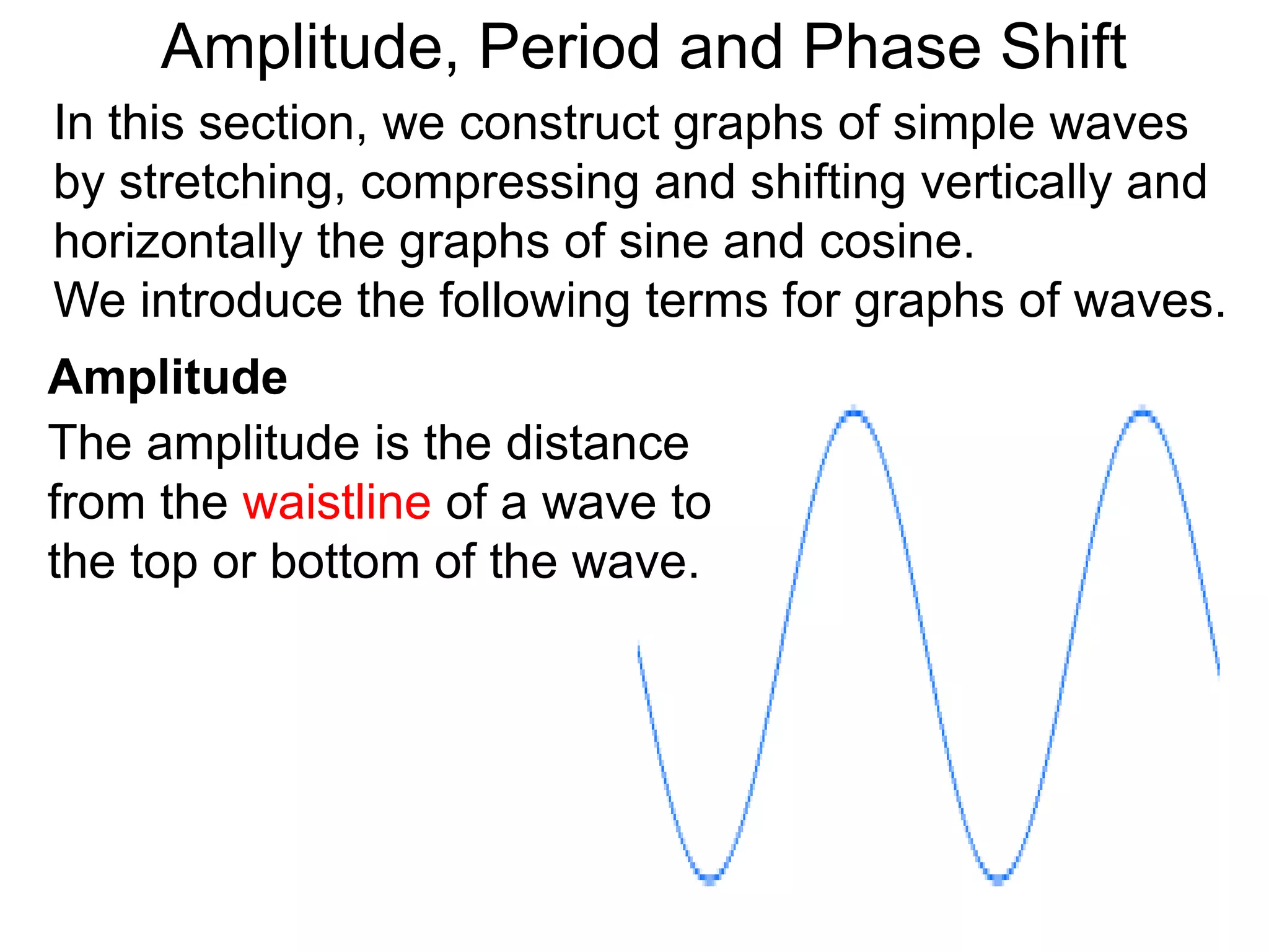
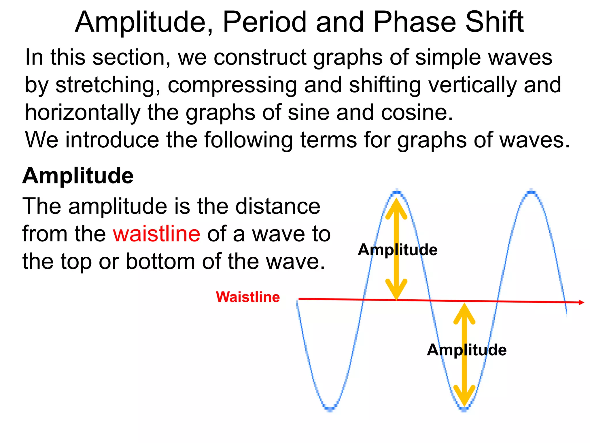
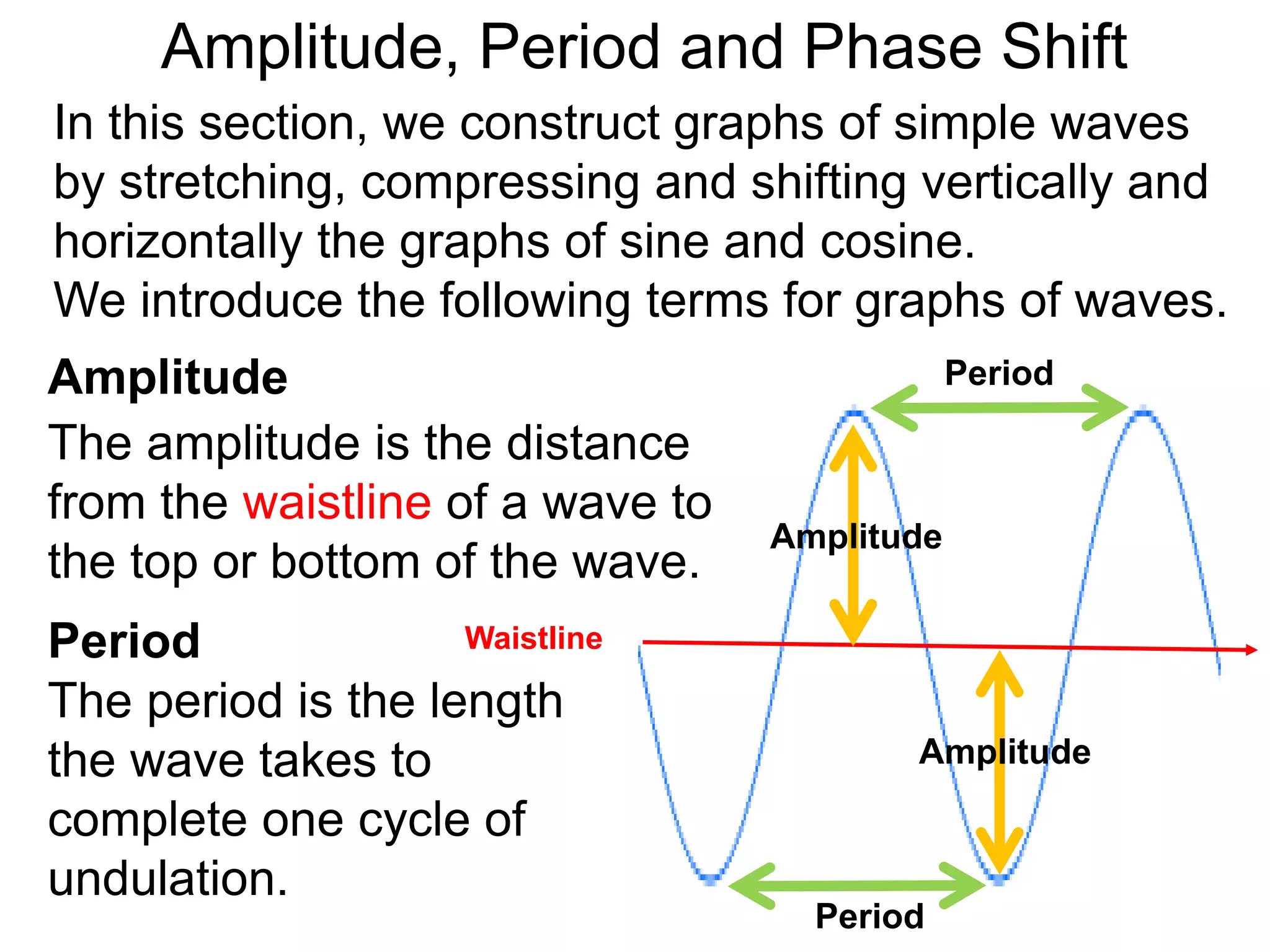
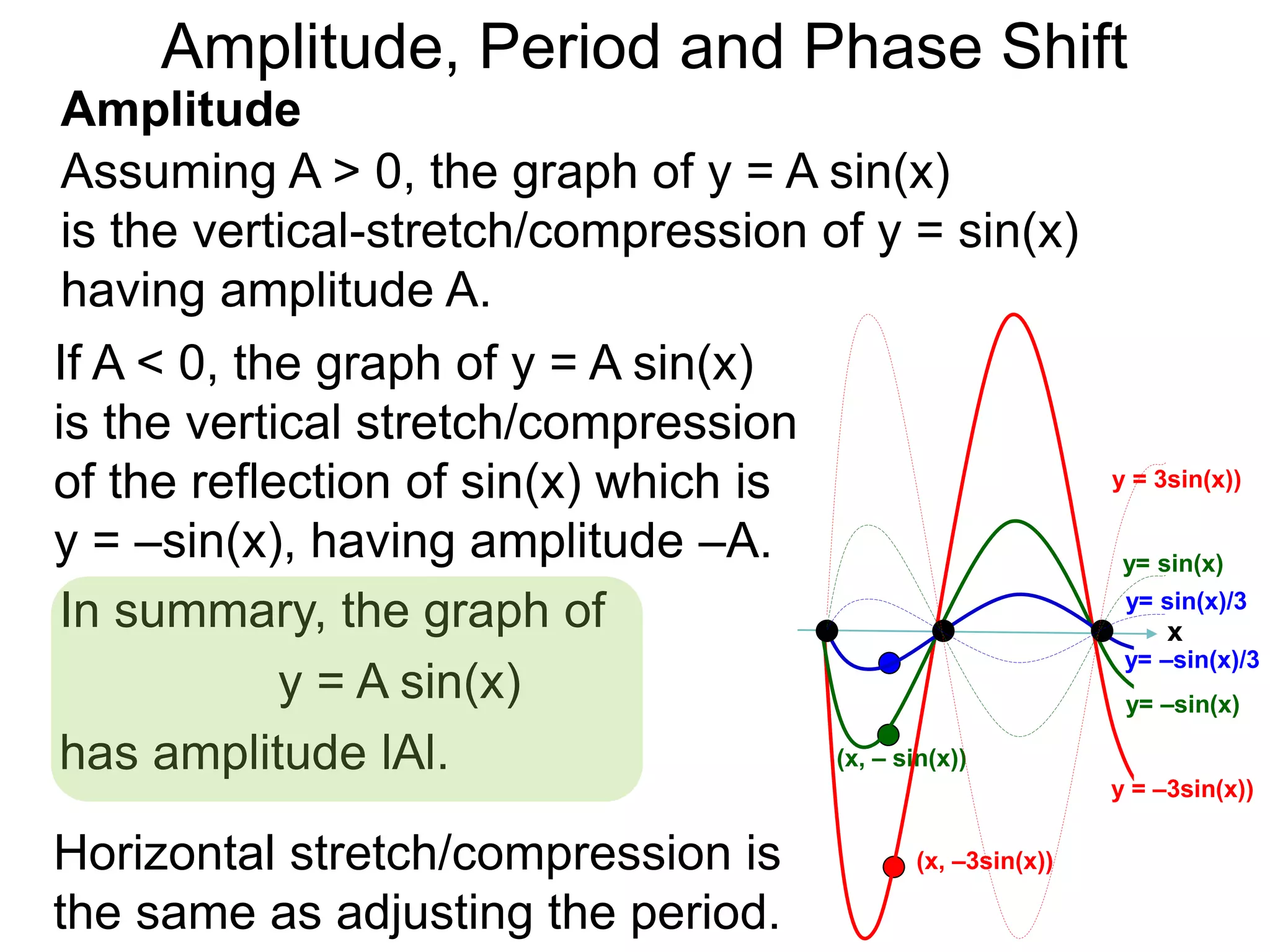
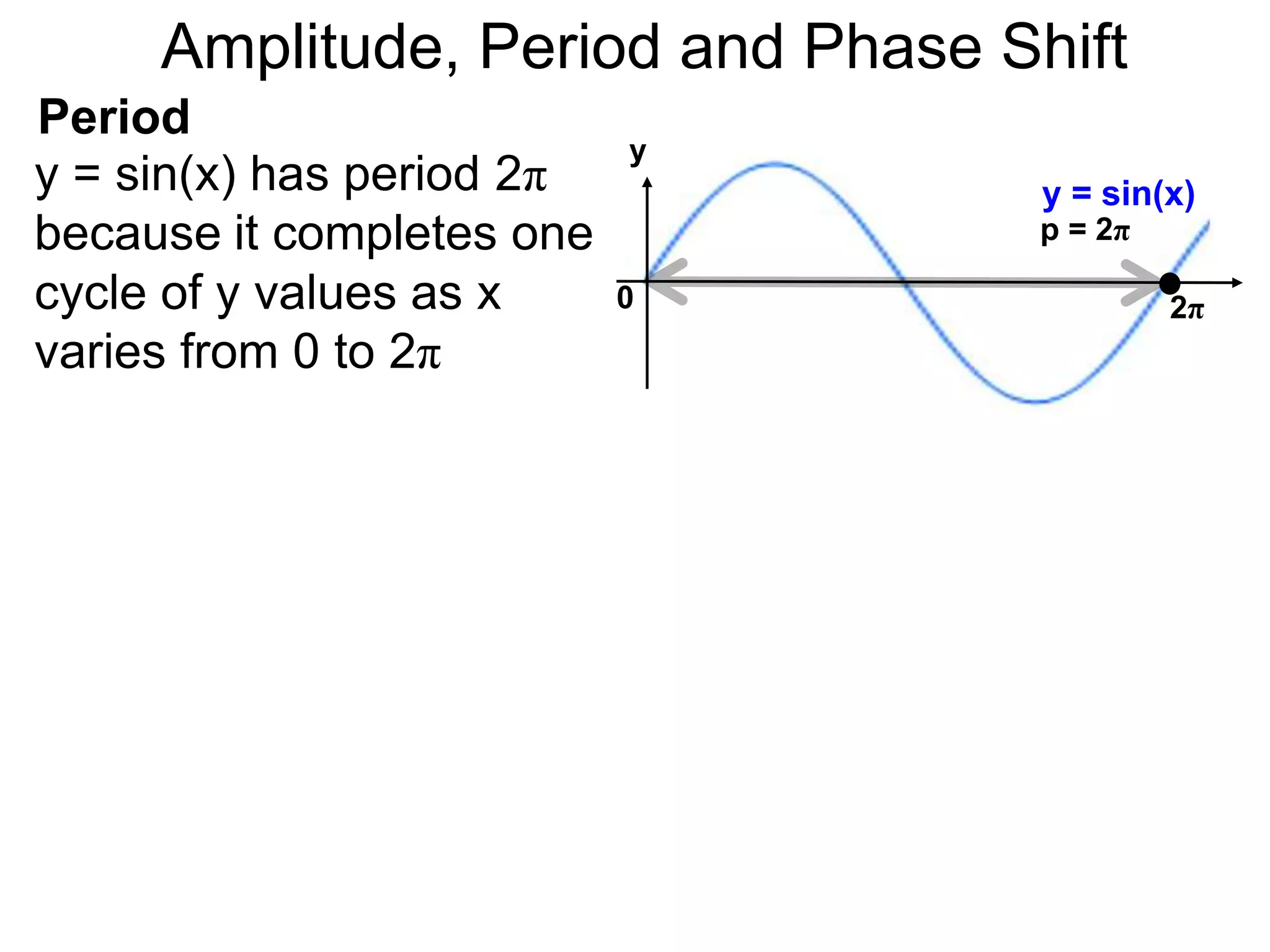
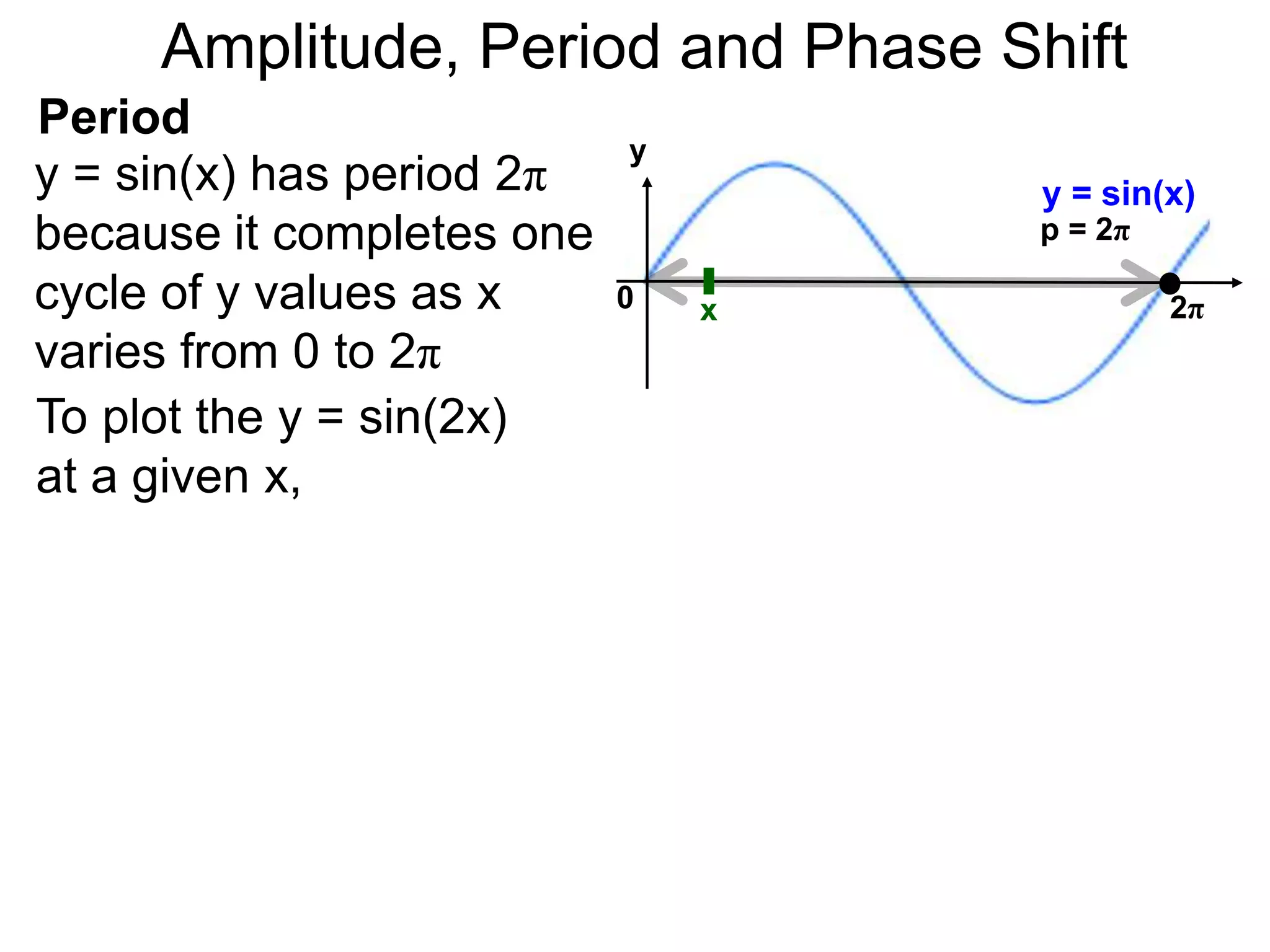
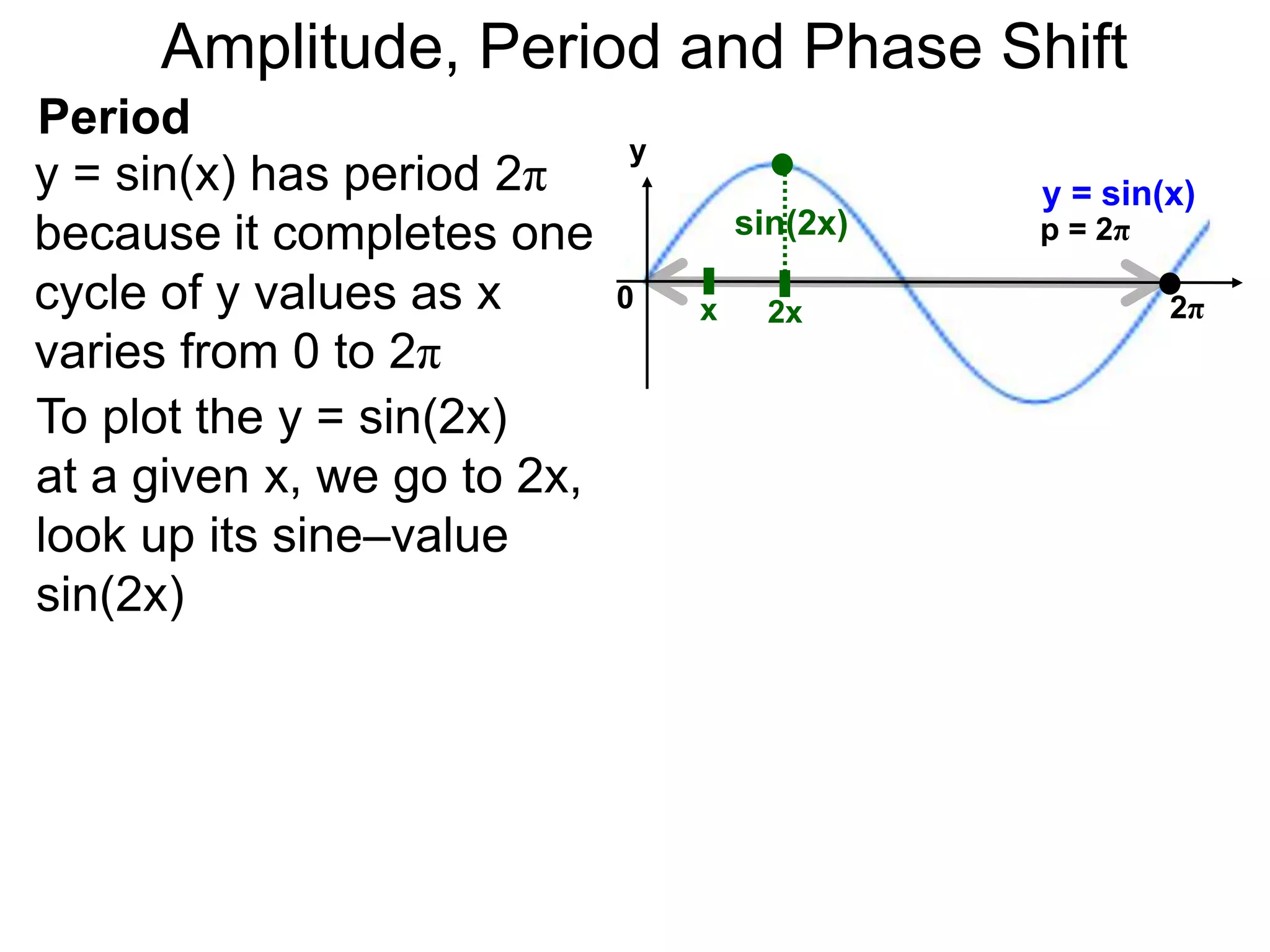
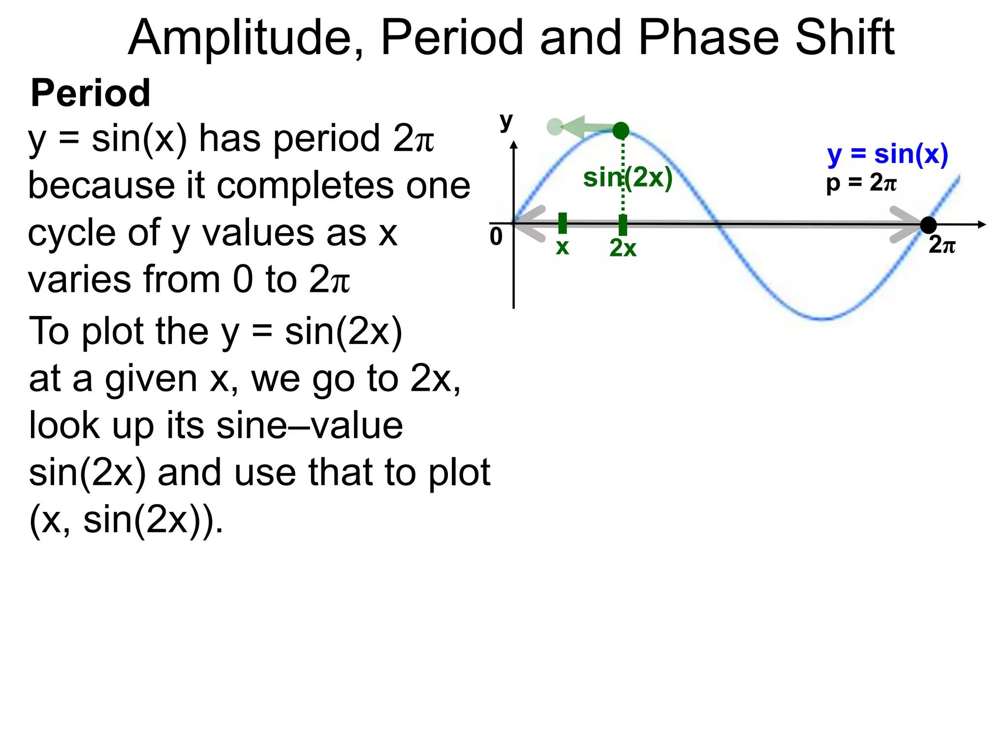
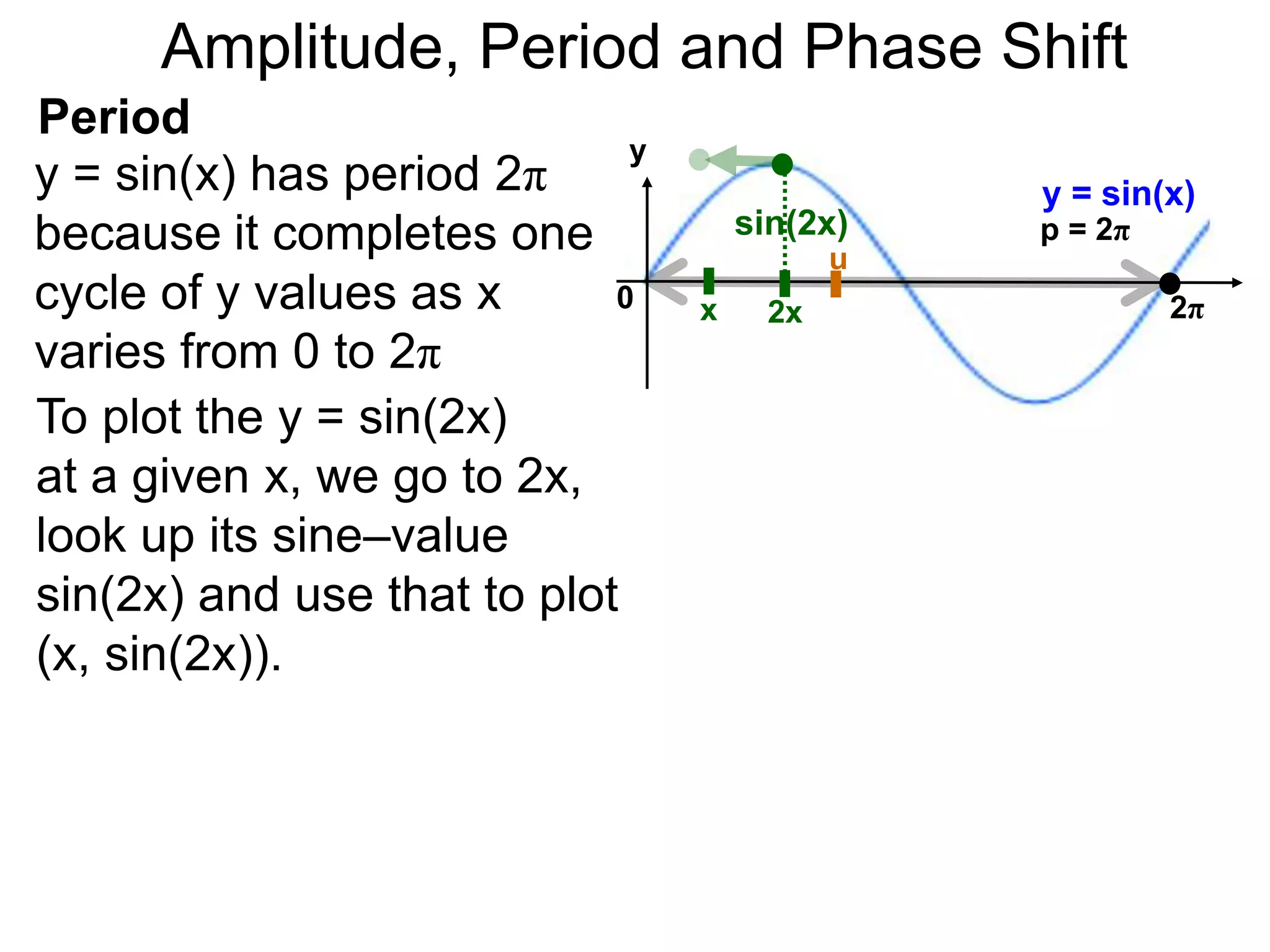
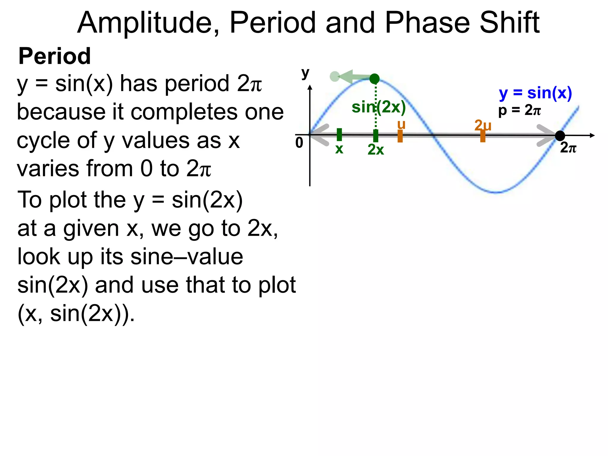
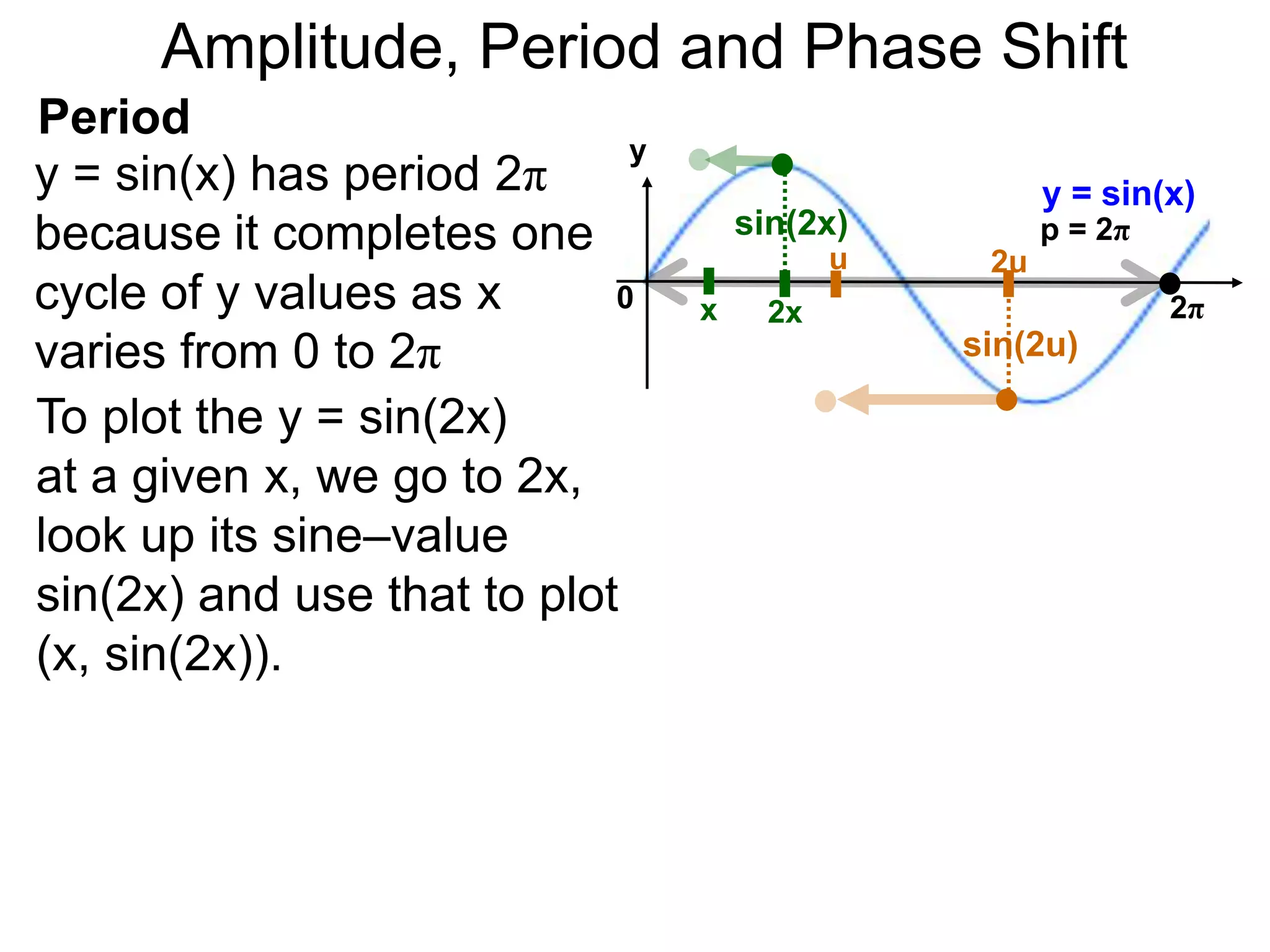
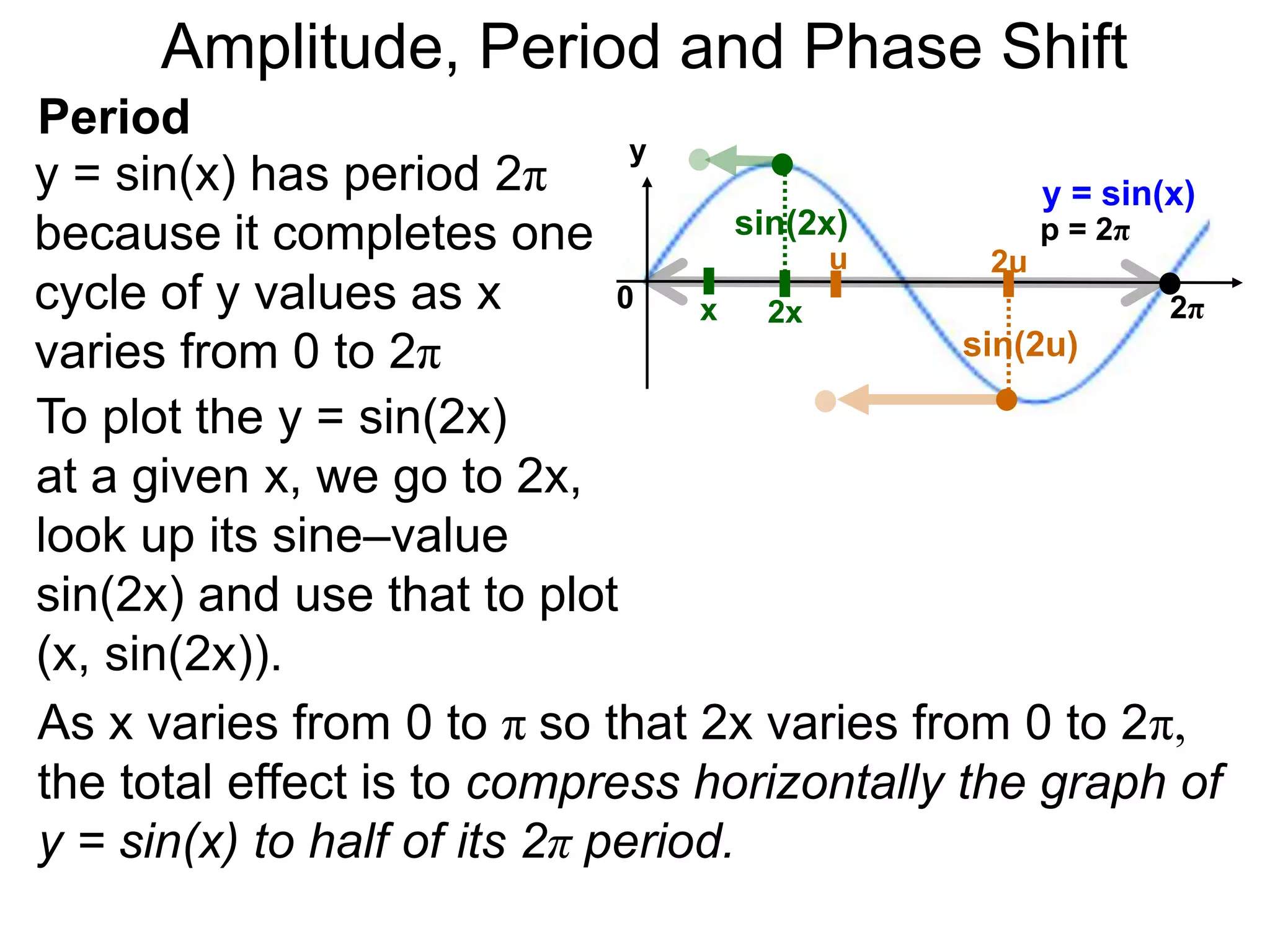
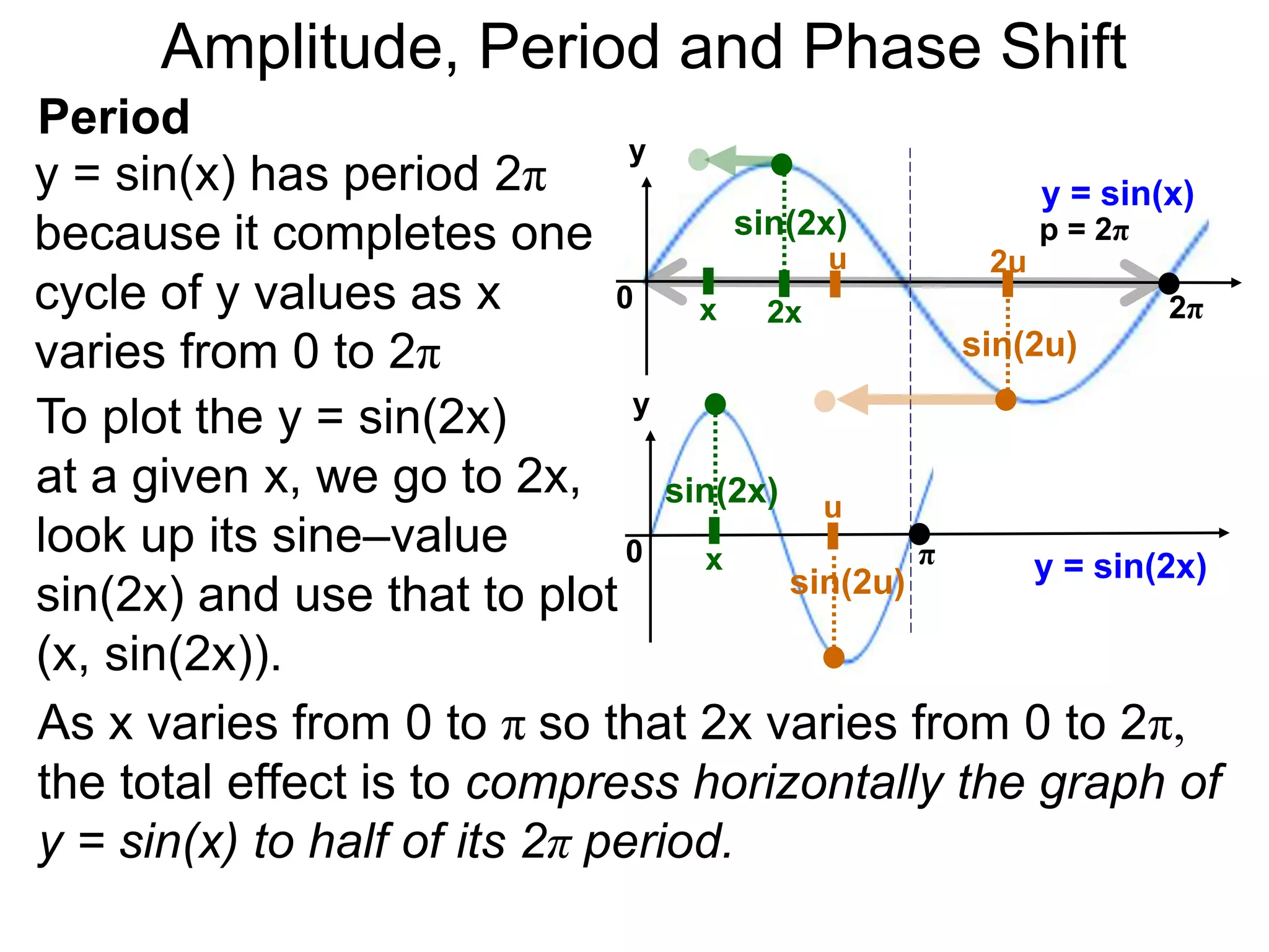
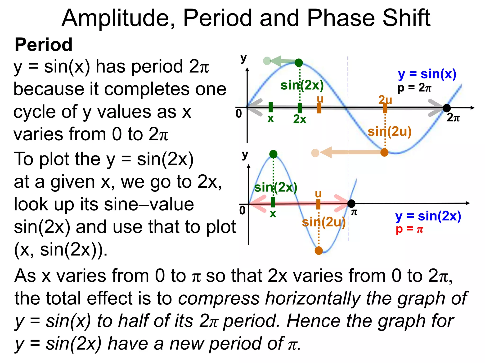
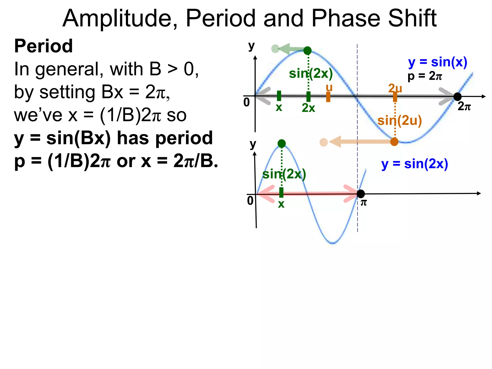
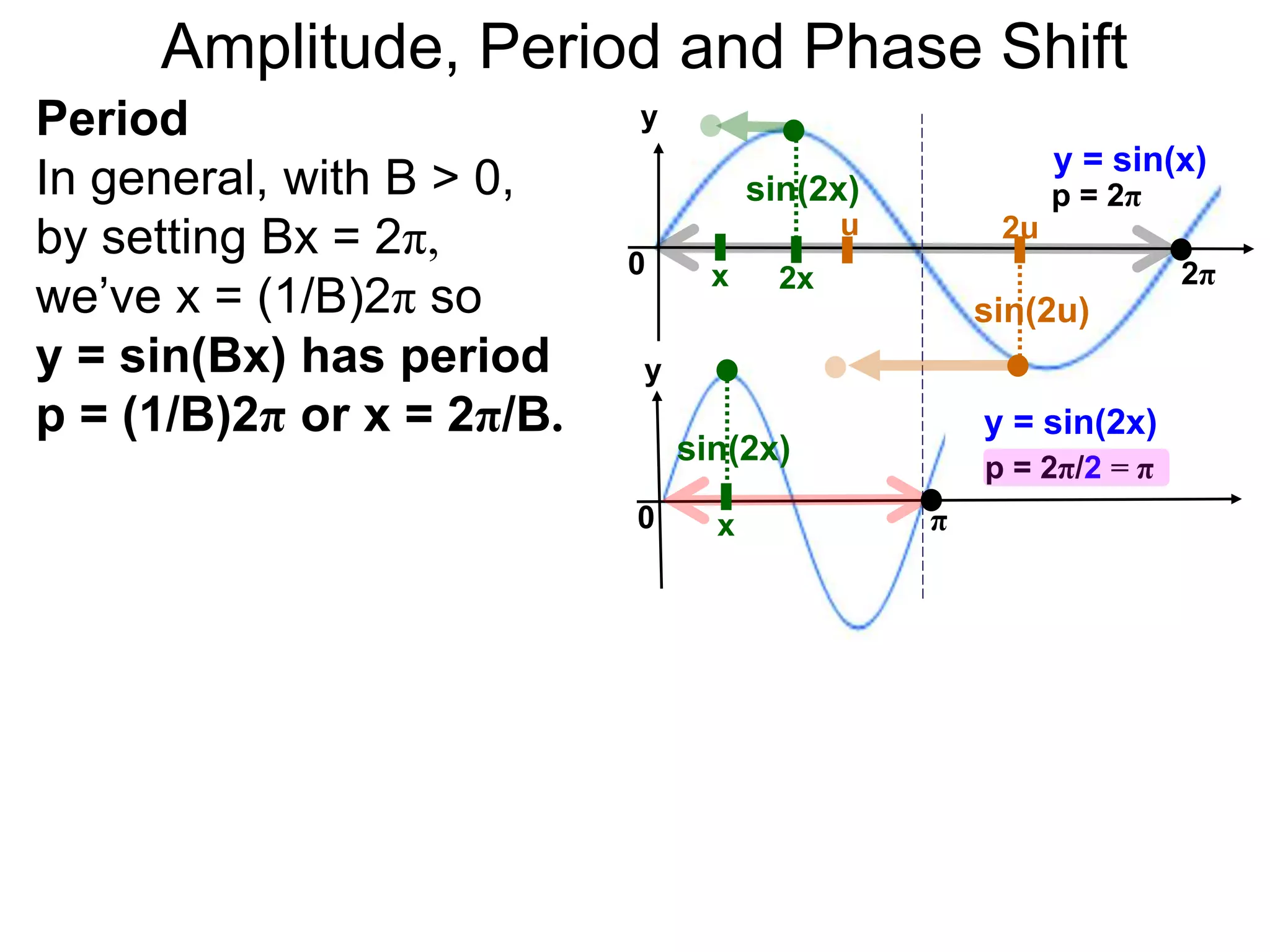
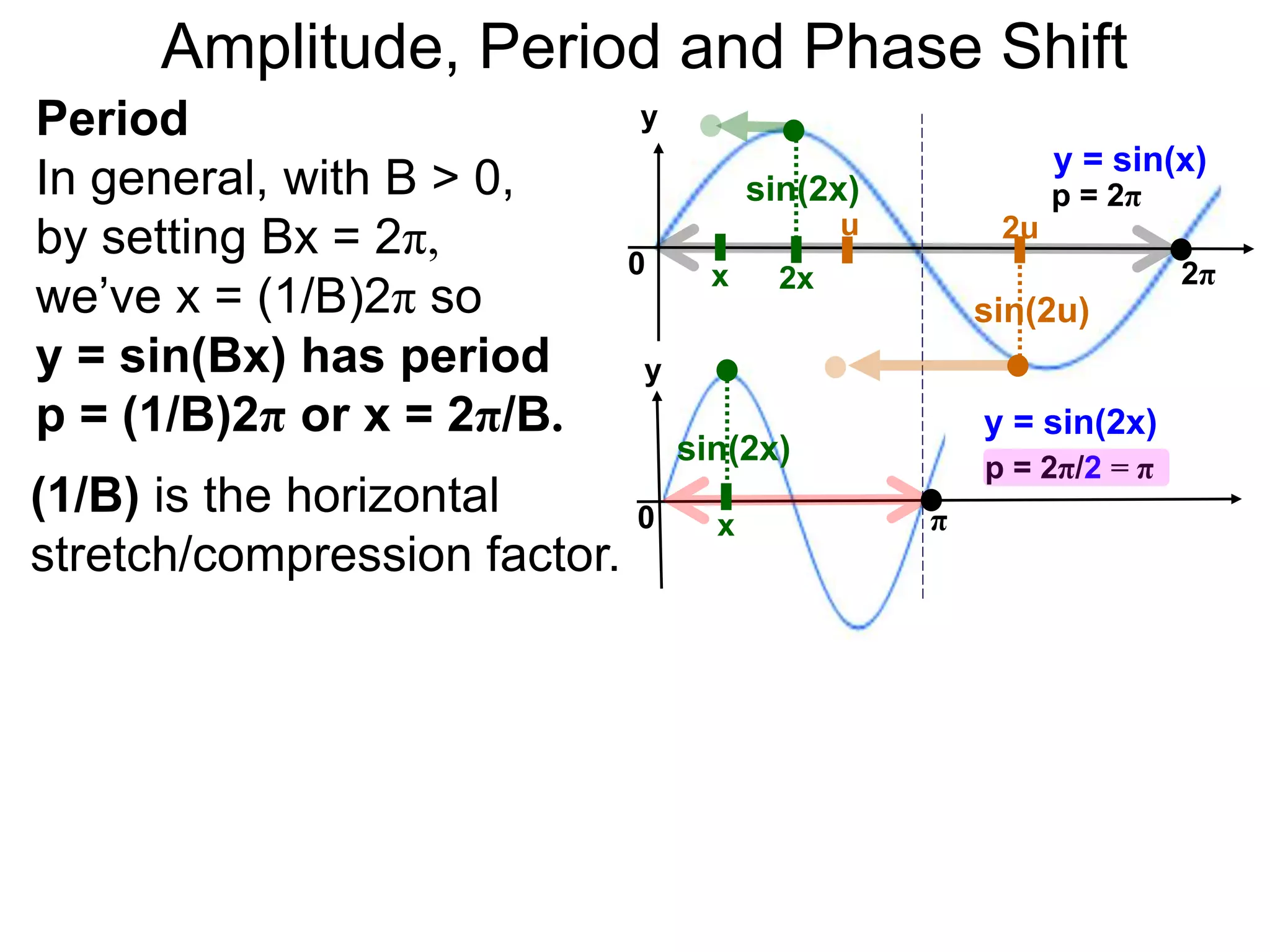
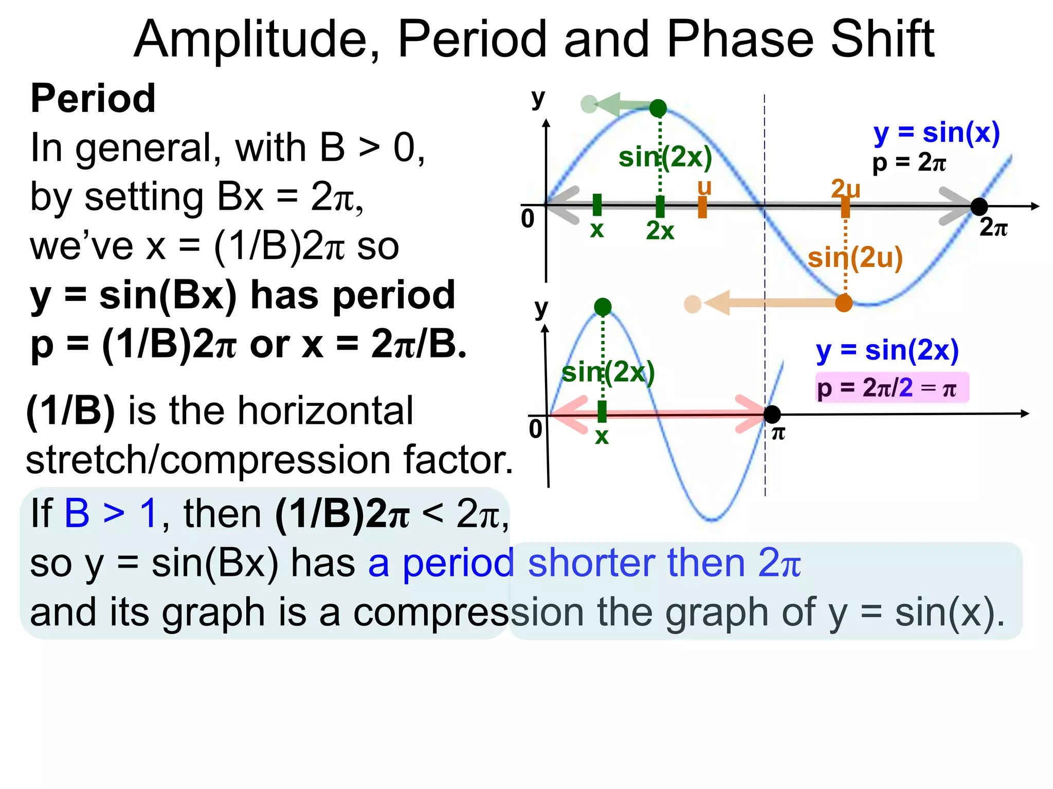
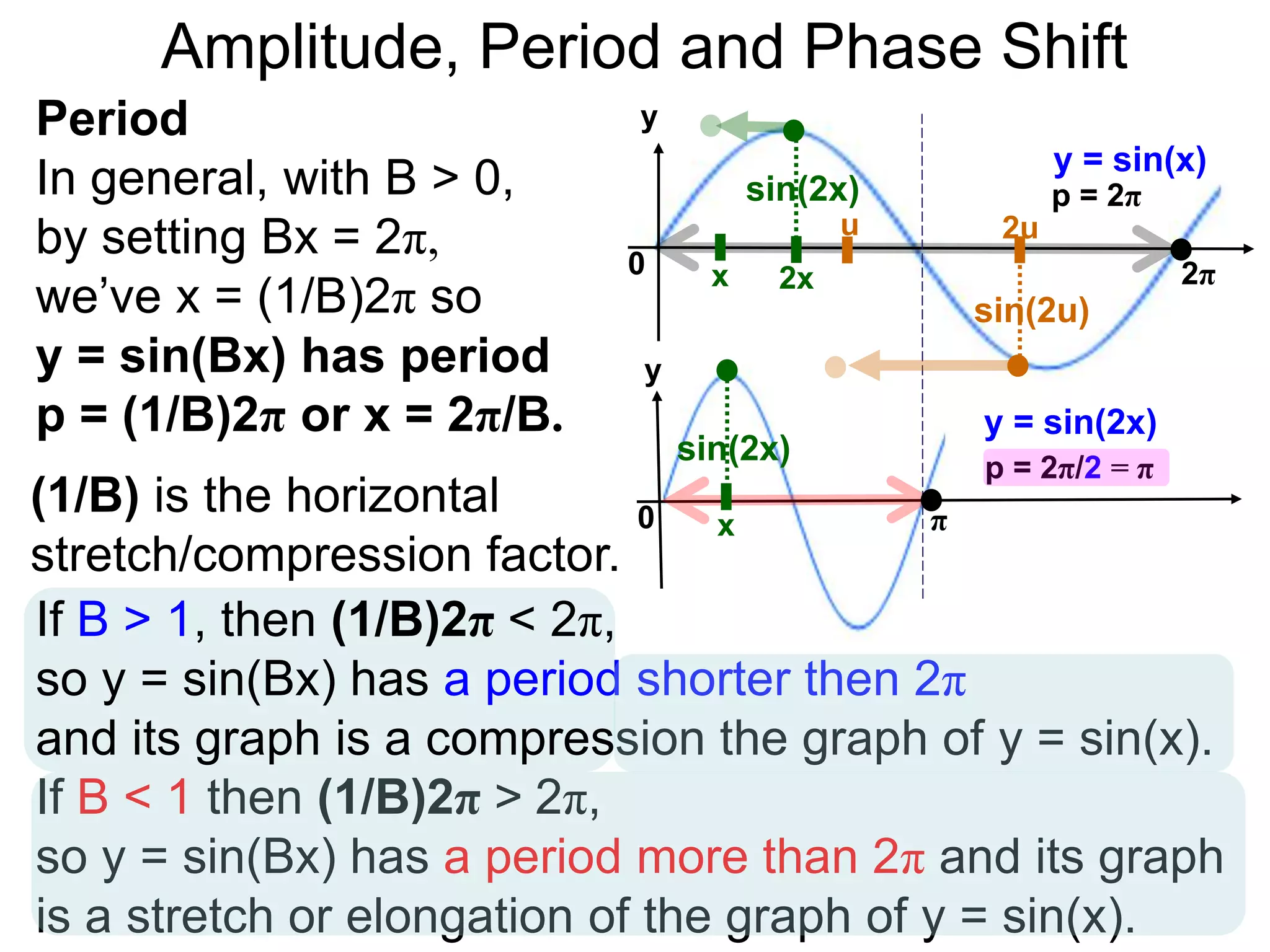
The document discusses amplitude, period, and phase shift of waves. It defines amplitude as the distance from the waistline of a wave to its peak or trough. Period is the length of time or space for a wave to complete one cycle. Vertically stretching or compressing a sine or cosine graph changes its amplitude. Horizontally compressing or stretching changes its period. For example, y=sin(2x) has half the period of y=sin(x) because as x varies from 0 to π, 2x varies from 0 to 2π, compressing the wave horizontally.

1. Amplitude, Period and Phase Shift

2. Amplitude, Period and Phase Shift
In this section, we construct graphs of simple waves
by stretching, compressing and shifting vertically and
horizontally the graphs of sine and cosine.

3. Amplitude, Period and Phase Shift
In this section, we construct graphs of simple waves
by stretching, compressing and shifting vertically and
horizontally the graphs of sine and cosine.
We introduce the following terms for graphs of waves.

4. Amplitude, Period and Phase Shift
Amplitude
In this section, we construct graphs of simple waves
by stretching, compressing and shifting vertically and
horizontally the graphs of sine and cosine.
We introduce the following terms for graphs of waves.
The amplitude is the distance
from the waistline of a wave to
the top or bottom of the wave.

5. Amplitude, Period and Phase Shift
Amplitude
In this section, we construct graphs of simple waves
by stretching, compressing and shifting vertically and
horizontally the graphs of sine and cosine.
We introduce the following terms for graphs of waves.
The amplitude is the distance
from the waistline of a wave to
the top or bottom of the wave.
Amplitude
Amplitude
Waistline

6. Amplitude, Period and Phase Shift
Amplitude
In this section, we construct graphs of simple waves
by stretching, compressing and shifting vertically and
horizontally the graphs of sine and cosine.
We introduce the following terms for graphs of waves.
The period is the length
the wave takes to
complete one cycle of
undulation.
Amplitude
Amplitude
Period
Period
Period Waistline
The amplitude is the distance
from the waistline of a wave to
the top or bottom of the wave.

7. Amplitude (Vertical Extension and Compression)
Amplitude, Period and Phase Shift

8. Given y = sin(x), and P = (x, sin(x)) a generic point
on the graph as shown,
Amplitude (Vertical Extension and Compression)
P = (x, sin(x))
y= sin(x)
sin(x)
x
Amplitude, Period and Phase Shift

9. Given y = sin(x), and P = (x, sin(x)) a generic point
on the graph as shown,
Amplitude (Vertical Extension and Compression)
P = (x, sin(x))
y= sin(x)
sin(x)
x
Amplitude, Period and Phase Shift

10. Given y = sin(x), and P = (x, sin(x)) a generic point
on the graph as shown, the graph of y = 3sin(x) at x
would yield the point (x, 3sin(x))
by tripling the height of the point P.
Amplitude (Vertical Extension and Compression)
P = (x, sin(x))
(x, 3sin(x))
y= sin(x)
sin(x)
x
Amplitude, Period and Phase Shift

11. Given y = sin(x), and P = (x, sin(x)) a generic point
on the graph as shown, the graph of y = 3sin(x) at x
would yield the point (x, 3sin(x))
by tripling the height of the point P.
Amplitude (Vertical Extension and Compression)
P = (x, sin(x))
Hence plotting y = 3sin(x) means
to elongate the entire graph
of y = sin(x) by 3 fold.
(x, 3sin(x))
y= sin(x)
y = 3sin(x))
sin(x)
x
Amplitude, Period and Phase Shift

12. Given y = sin(x), and P = (x, sin(x)) a generic point
on the graph as shown, the graph of y = 3sin(x) at x
would yield the point (x, 3sin(x))
by tripling the height of the point P.
Amplitude (Vertical Extension and Compression)
P = (x, sin(x))
Hence plotting y = 3sin(x) means
to elongate the entire graph
of y = sin(x) by 3 fold while
the x–intercepts or (x, 0)’s
remain fixed because 3(0) = 0.
(x, 3sin(x))
y= sin(x)
y = 3sin(x))
sin(x)
x
Amplitude, Period and Phase Shift

13. Given y = sin(x), and P = (x, sin(x)) a generic point
on the graph as shown, the graph of y = 3sin(x) at x
would yield the point (x, 3sin(x))
by tripling the height of the point P.
Amplitude (Vertical Extension and Compression)
P = (x, sin(x))
Hence plotting y = 3sin(x) means
to elongate the entire graph
of y = sin(x) by 3 fold while
the x–intercepts or (x, 0)’s
remain fixed because 3(0) = 0.
Likewise setting y = (1/3)sin(x) would
compress vertically the entire graph
to a third of its original height while
the x–intercepts or (x, 0)’s remain fixed.
(x, 3sin(x))
y= sin(x)
y= sin(x)/3
y = 3sin(x))
sin(x)
x
Amplitude, Period and Phase Shift

14. Amplitude
Assuming A > 0, the graph of y = A sin(x)
is the vertical-stretch/compression of y = sin(x)
having amplitude A.
Amplitude, Period and Phase Shift

15. Amplitude
Assuming A > 0, the graph of y = A sin(x)
is the vertical-stretch/compression of y = sin(x)
having amplitude A.
x
y= sin(x)
y = 3sin(x))
y= sin(x)/3
Amplitude, Period and Phase Shift

16. Amplitude
Assuming A > 0, the graph of y = A sin(x)
is the vertical-stretch/compression of y = sin(x)
having amplitude A.
If A < 0, the graph of y = A sin(x)
is the vertical stretch/compression
of the reflection of sin(x) which is
y = –sin(x), having amplitude –A.
(x, – sin(x))
(x, –3sin(x))
x
y= –sin(x)
y = –3sin(x))
y= –sin(x)/3
y= sin(x)
y = 3sin(x))
y= sin(x)/3
Amplitude, Period and Phase Shift

17. Amplitude
Assuming A > 0, the graph of y = A sin(x)
is the vertical-stretch/compression of y = sin(x)
having amplitude A.
(x, – sin(x))
(x, –3sin(x))
x
y= –sin(x)
y = –3sin(x))
y= –sin(x)/3
In summary, the graph of
y = A sin(x)
has amplitude lAl.
y= sin(x)
y = 3sin(x))
y= sin(x)/3
If A < 0, the graph of y = A sin(x)
is the vertical stretch/compression
of the reflection of sin(x) which is
y = –sin(x), having amplitude –A.
Amplitude, Period and Phase Shift

18. Amplitude
Assuming A > 0, the graph of y = A sin(x)
is the vertical-stretch/compression of y = sin(x)
having amplitude A.
(x, – sin(x))
(x, –3sin(x))
x
y= –sin(x)
y = –3sin(x))
y= –sin(x)/3
In summary, the graph of
y = A sin(x)
has amplitude lAl.
Horizontal stretch/compression is
the same as adjusting the period.
y= sin(x)
y = 3sin(x))
y= sin(x)/3
If A < 0, the graph of y = A sin(x)
is the vertical stretch/compression
of the reflection of sin(x) which is
y = –sin(x), having amplitude –A.
Amplitude, Period and Phase Shift

19. Amplitude, Period and Phase Shift
Period

20. Amplitude, Period and Phase Shift
Period
y = sin(x) has period 2π
because it completes one
cycle of y values as x
varies from 0 to 2π
y
y = sin(x)
p = 2π
0 2π

21. Amplitude, Period and Phase Shift
Period
y = sin(x) has period 2π
because it completes one
cycle of y values as x
varies from 0 to 2π
y
y = sin(x)
p = 2π
0 2π

22. Amplitude, Period and Phase Shift
Period
y = sin(x) has period 2π
because it completes one
cycle of y values as x
varies from 0 to 2π
y
y = sin(x)
p = 2π
0 2π
To plot the y = sin(2x)
at a given x,
x

23. Amplitude, Period and Phase Shift
Period
y = sin(x) has period 2π
because it completes one
cycle of y values as x
varies from 0 to 2π
y
y = sin(x)
p = 2π
0 2π
To plot the y = sin(2x)
at a given x, we go to 2x,
look up its sine–value
sin(2x)
x 2x
sin(2x)

24. Amplitude, Period and Phase Shift
Period
y = sin(x) has period 2π
because it completes one
cycle of y values as x
varies from 0 to 2π
y
y = sin(x)
p = 2π
0 2π
To plot the y = sin(2x)
at a given x, we go to 2x,
look up its sine–value
sin(2x) and use that to plot
(x, sin(2x)).
x 2x
sin(2x)

25. Amplitude, Period and Phase Shift
Period
y = sin(x) has period 2π
because it completes one
cycle of y values as x
varies from 0 to 2π
y
y = sin(x)
p = 2π
0 2π
To plot the y = sin(2x)
at a given x, we go to 2x,
look up its sine–value
sin(2x) and use that to plot
(x, sin(2x)).
x 2x
sin(2x)
u

26. Amplitude, Period and Phase Shift
Period
y = sin(x) has period 2π
because it completes one
cycle of y values as x
varies from 0 to 2π
y
y = sin(x)
p = 2π
0 2π
To plot the y = sin(2x)
at a given x, we go to 2x,
look up its sine–value
sin(2x) and use that to plot
(x, sin(2x)).
x 2x
sin(2x)
2uu

27. Amplitude, Period and Phase Shift
Period
y = sin(x) has period 2π
because it completes one
cycle of y values as x
varies from 0 to 2π
y
y = sin(x)
p = 2π
0 2π
To plot the y = sin(2x)
at a given x, we go to 2x,
look up its sine–value
sin(2x) and use that to plot
(x, sin(2x)).
x 2x
sin(2x)
2uu
sin(2u)

28. Amplitude, Period and Phase Shift
Period
y = sin(x) has period 2π
because it completes one
cycle of y values as x
varies from 0 to 2π
y
y = sin(x)
p = 2π
0 2π
To plot the y = sin(2x)
at a given x, we go to 2x,
look up its sine–value
sin(2x) and use that to plot
(x, sin(2x)).
As x varies from 0 to π so that 2x varies from 0 to 2π,
the total effect is to compress horizontally the graph of
y = sin(x) to half of its 2π period.
x 2x
sin(2x)
2uu
sin(2u)

29. Amplitude, Period and Phase Shift
Period
y = sin(x) has period 2π
because it completes one
cycle of y values as x
varies from 0 to 2π
y
y = sin(x)
p = 2π
0 2π
To plot the y = sin(2x)
at a given x, we go to 2x,
look up its sine–value
sin(2x) and use that to plot
(x, sin(2x)).
As x varies from 0 to π so that 2x varies from 0 to 2π,
the total effect is to compress horizontally the graph of
y = sin(x) to half of its 2π period.
y
y = sin(2x)0 π
x
x
2x
sin(2x)
sin(2x) u
2u
sin(2u)
u
sin(2u)

30. Amplitude, Period and Phase Shift
Period
y = sin(x) has period 2π
because it completes one
cycle of y values as x
varies from 0 to 2π
y
y = sin(x)
p = 2π
0 2π
To plot the y = sin(2x)
at a given x, we go to 2x,
look up its sine–value
sin(2x) and use that to plot
(x, sin(2x)).
As x varies from 0 to π so that 2x varies from 0 to 2π,
the total effect is to compress horizontally the graph of
y = sin(x) to half of its 2π period. Hence the graph for
y = sin(2x) have a new period of π.
y
y = sin(2x)0
p = π
π
x
x
2x
sin(2x)
sin(2x) u
2u
sin(2u)
u
sin(2u)

31. Amplitude, Period and Phase Shift
Period
In general, with B > 0,
by setting Bx = 2π,
we’ve x = (1/B)2π so
y = sin(Bx) has period
p = (1/B)2π or x = 2π/B.
y
y = sin(x)
p = 2π
0 2π
y
y = sin(2x)
0 π
x
x
2x
sin(2x)
sin(2x)
2uu
sin(2u)

32. Amplitude, Period and Phase Shift
Period
In general, with B > 0,
by setting Bx = 2π,
we’ve x = (1/B)2π so
y = sin(Bx) has period
p = (1/B)2π or x = 2π/B.
y
y = sin(x)
p = 2π
0 2π
y
y = sin(2x)
0
p = 2π/2 = π
π
x
x
2x
sin(2x)
sin(2x)
2uu
sin(2u)

33. Amplitude, Period and Phase Shift
Period
In general, with B > 0,
by setting Bx = 2π,
we’ve x = (1/B)2π so
y = sin(Bx) has period
p = (1/B)2π or x = 2π/B.
y
y = sin(x)
p = 2π
0 2π
y
y = sin(2x)
0 π
x
x
2x
sin(2x)
sin(2x)
2uu
sin(2u)
(1/B) is the horizontal
stretch/compression factor.
p = 2π/2 = π

34. Amplitude, Period and Phase Shift
Period
In general, with B > 0,
by setting Bx = 2π,
we’ve x = (1/B)2π so
y = sin(Bx) has period
p = (1/B)2π or x = 2π/B.
y
y = sin(x)
p = 2π
0 2π
y
y = sin(2x)
0 π
x
x
2x
sin(2x)
sin(2x)
2uu
sin(2u)
(1/B) is the horizontal
stretch/compression factor.
If B > 1, then (1/B)2π < 2π,
so y = sin(Bx) has a period shorter then 2π
and its graph is a compression the graph of y = sin(x).
p = 2π/2 = π

35. Amplitude, Period and Phase Shift
Period
In general, with B > 0,
by setting Bx = 2π,
we’ve x = (1/B)2π so
y = sin(Bx) has period
p = (1/B)2π or x = 2π/B.
y
y = sin(x)
p = 2π
0 2π
y
y = sin(2x)
0 π
x
x
2x
sin(2x)
sin(2x)
2uu
sin(2u)
(1/B) is the horizontal
stretch/compression factor.
If B > 1, then (1/B)2π < 2π,
so y = sin(Bx) has a period shorter then 2π
and its graph is a compression the graph of y = sin(x).
If B < 1 then (1/B)2π > 2π,
so y = sin(Bx) has a period more than 2π and its graph
is a stretch or elongation of the graph of y = sin(x).
p = 2π/2 = π

36. Given the point (x, y), (x, y + 1)
is 1 units above it so the point
(x, sin(x) + 1) is 1 unit up from
(x, sin(x)).
Amplitude, Period and Phase Shift

37. y= sin(x)
Given the point (x, y), (x, y + 1)
is 1 units above it so the point
(x, sin(x) + 1) is 1 unit up from
(x, sin(x)).
(x, sin(x)+1)
x(x, sin(x))
Amplitude, Period and Phase Shift

38. y= sin(x)
Given the point (x, y), (x, y + 1)
is 1 units above it so the point
(x, sin(x) + 1) is 1 unit up from
(x, sin(x)). Hence the graph of
y = sin(x) + 1 is 1 unit up
from the graph of y = sin(x).
(x, sin(x)+1)
y= sin(x) + 1
x(x, sin(x))
2
Amplitude, Period and Phase Shift

39. y= sin(x)
Given the point (x, y), (x, y + 1)
is 1 units above it so the point
(x, sin(x) + 1) is 1 unit up from
(x, sin(x)). Hence the graph of
y = sin(x) + 1 is 1 unit up
from the graph of y = sin(x).
(x, sin(x)+1)
y= sin(x) + 1
x(x, sin(x))
Similarly, the point (x, y – 1)
is 1 units below (x, y)
2
Amplitude, Period and Phase Shift

40. y= sin(x)
Given the point (x, y), (x, y + 1)
is 1 units above it so the point
(x, sin(x) + 1) is 1 unit up from
(x, sin(x)). Hence the graph of
y = sin(x) + 1 is 1 unit up
from the graph of y = sin(x).
(x, sin(x)+1)
(x, sin(x)–1)
y= sin(x) + 1
x(x, sin(x))
Similarly, the point (x, y – 1)
is 1 units below (x, y) so (x, sin(x) – 1) is 1 unit down
from (x, sin(x)).
2
Amplitude, Period and Phase Shift

41. y= sin(x)
Given the point (x, y), (x, y + 1)
is 1 units above it so the point
(x, sin(x) + 1) is 1 unit up from
(x, sin(x)). Hence the graph of
y = sin(x) + 1 is 1 unit up
from the graph of y = sin(x).
(x, sin(x)+1)
(x, sin(x)–1)
y= sin(x) – 1
y= sin(x) + 1
x(x, sin(x))
Similarly, the point (x, y – 1)
is 1 units below (x, y) so (x, sin(x) – 1) is 1 unit down
from (x, sin(x)). Correspondingly, the graph of
y = sin(x) – 1 is the graph of y = sin(x) 1 unit lowered.
2
–2
Amplitude, Period and Phase Shift

42. y= sin(x)
Vertical Translations (In reference to graphs)
Given the point (x, y), (x, y + 1)
is 1 units above it so the point
(x, sin(x) + 1) is 1 unit up from
(x, sin(x)). Hence the graph of
y = sin(x) + 1 is 1 unit up
from the graph of y = sin(x).
(x, sin(x)+1)
(x, sin(x)–1)
y= sin(x) – 1
y= sin(x) + 1
x(x, sin(x))
Similarly, the point (x, y – 1)
is 1 units below (x, y) so (x, sin(x) – 1) is 1 unit down
from (x, sin(x)). Correspondingly, the graph of
y = sin(x) – 1 is the graph of y = sin(x) 1 unit lowered.
y = sin(x) + C is the vertical translation of y = sin(x).
If C > 0, y = sin(x) + C is C unit up from y = sin(x).
2
–2
Amplitude, Period and Phase Shift

43. y= sin(x)
Vertical Translations (In reference to graphs)
Given the point (x, y), (x, y + 1)
is 1 units above it so the point
(x, sin(x) + 1) is 1 unit up from
(x, sin(x)). Hence the graph of
y = sin(x) + 1 is 1 unit up
from the graph of y = sin(x).
(x, sin(x)+1)
(x, sin(x)–1)
y= sin(x) – 1
y= sin(x) + 1
x(x, sin(x))
Similarly, the point (x, y – 1)
is 1 units below (x, y) so (x, sin(x) – 1) is 1 unit down
from (x, sin(x)). Correspondingly, the graph of
y = sin(x) – 1 is the graph of y = sin(x) 1 unit lowered.
y = sin(x) + C is the vertical translation of y = sin(x).
If C > 0, y = sin(x) + C is C unit up from y = sin(x).
If C < 0, y = sin(x) + C is C unit down from y = sin(x).
2
–2
Amplitude, Period and Phase Shift

44. Because the graph of y = sin(x) + C is the
vertical translation of y = sin(x) by C unit,
whose waistline y = 0 is moved to y = C
which is the waistline of y = sin(x) + C.
y
x
Move by C
waistline
y = 0
Amplitude, Period and Phase Shift

45. Because the graph of y = sin(x) + C is the
vertical translation of y = sin(x) by C unit,
whose waistline y = 0 is moved to y = C
which is the waistline of y = sin(x) + C.
y
x
Move by C
waistline
y = 0
waistline
y = C
Amplitude, Period and Phase Shift

46. Amplitude lAl
waistline
y = C
Because the graph of y = sin(x) + C is the
vertical translation of y = sin(x) by C unit,
whose waistline y = 0 is moved to y = C
which is the waistline of y = sin(x) + C.
In particular since y = Asin(x) + C has amplitude lAl,
y = Asin(x) + C
y
x
y = Asin(x)
Move by C
waistline
y = 0
Amplitude, Period and Phase Shift

47. Amplitude lAl
waistline
y = C
Because the graph of y = sin(x) + C is the
vertical translation of y = sin(x) by C unit,
whose waistline y = 0 is moved to y = C
which is the waistline of y = sin(x) + C.
In particular since y = Asin(x) + C has amplitude lAl,
so y ranges from y = C – lAl to y = C + lAl.
y = C+lAl
y = C–lAl
y = Asin(x) + C
y
x
y = Asin(x)
Move by C
waistline
y = 0
Amplitude, Period and Phase Shift

48. Amplitude, Period and Phase Shift
Example B.
Sketch graph of y = –3sin(x/2) + 5.
List the period and the amplitude. Draw the waistline
and the range of y.

49. The amplitude is 3 and the period is [1/(1/2)] 2π = 4π.
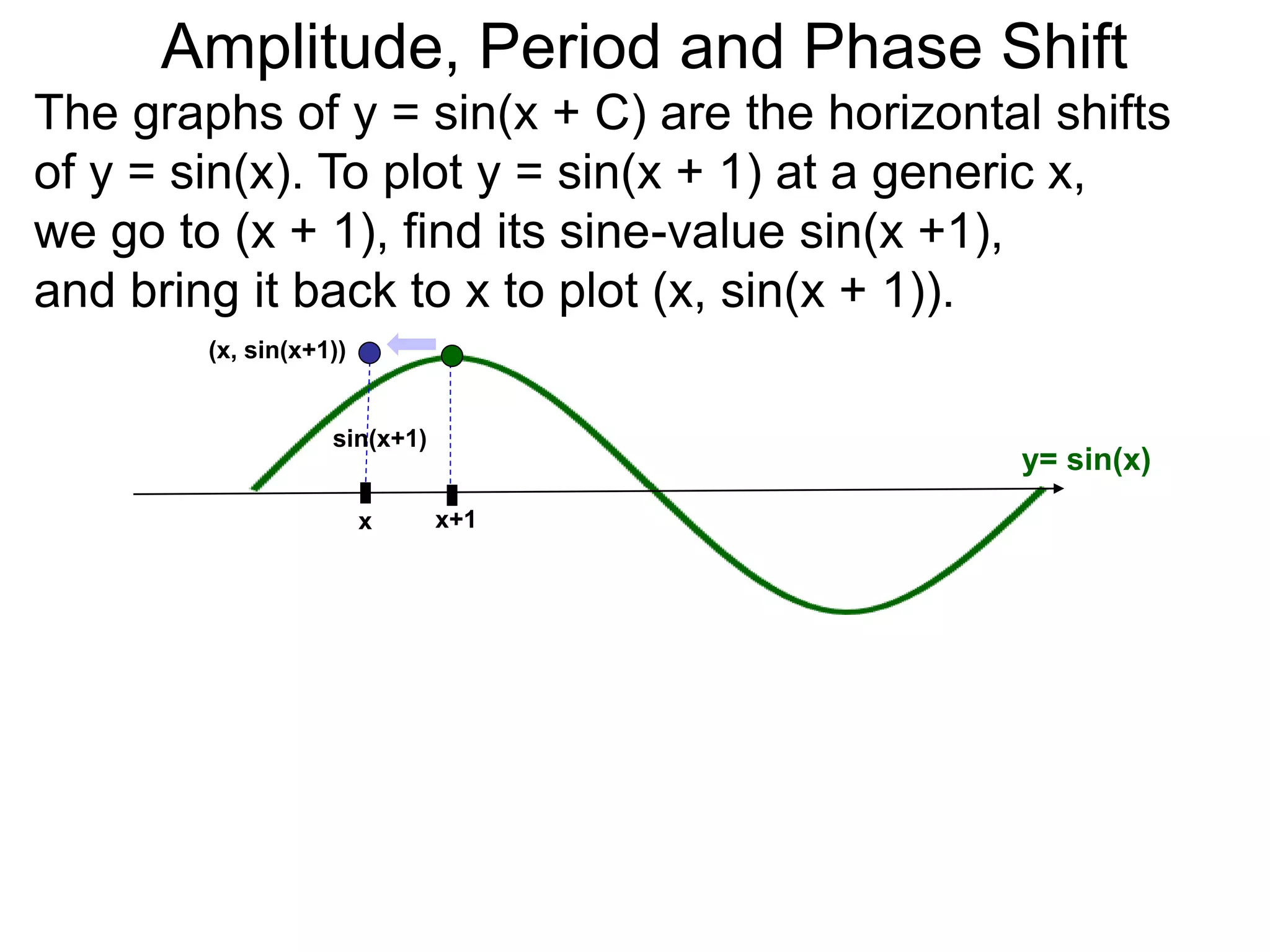
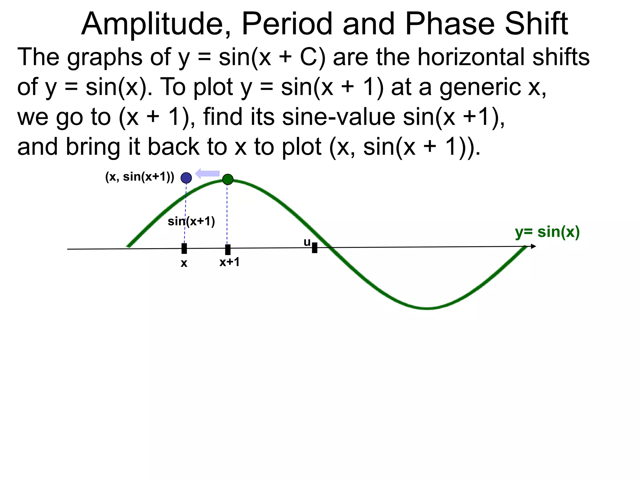
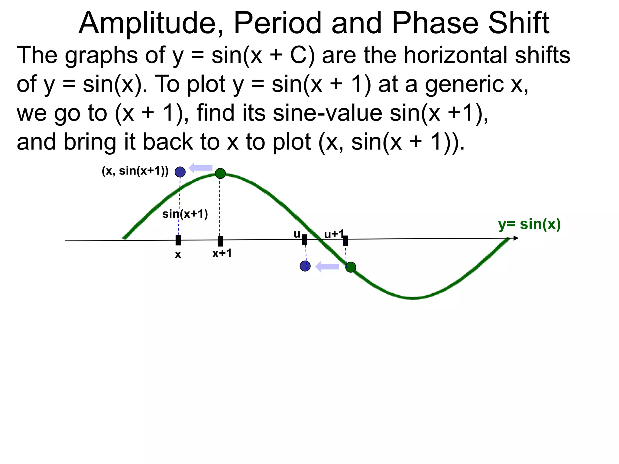
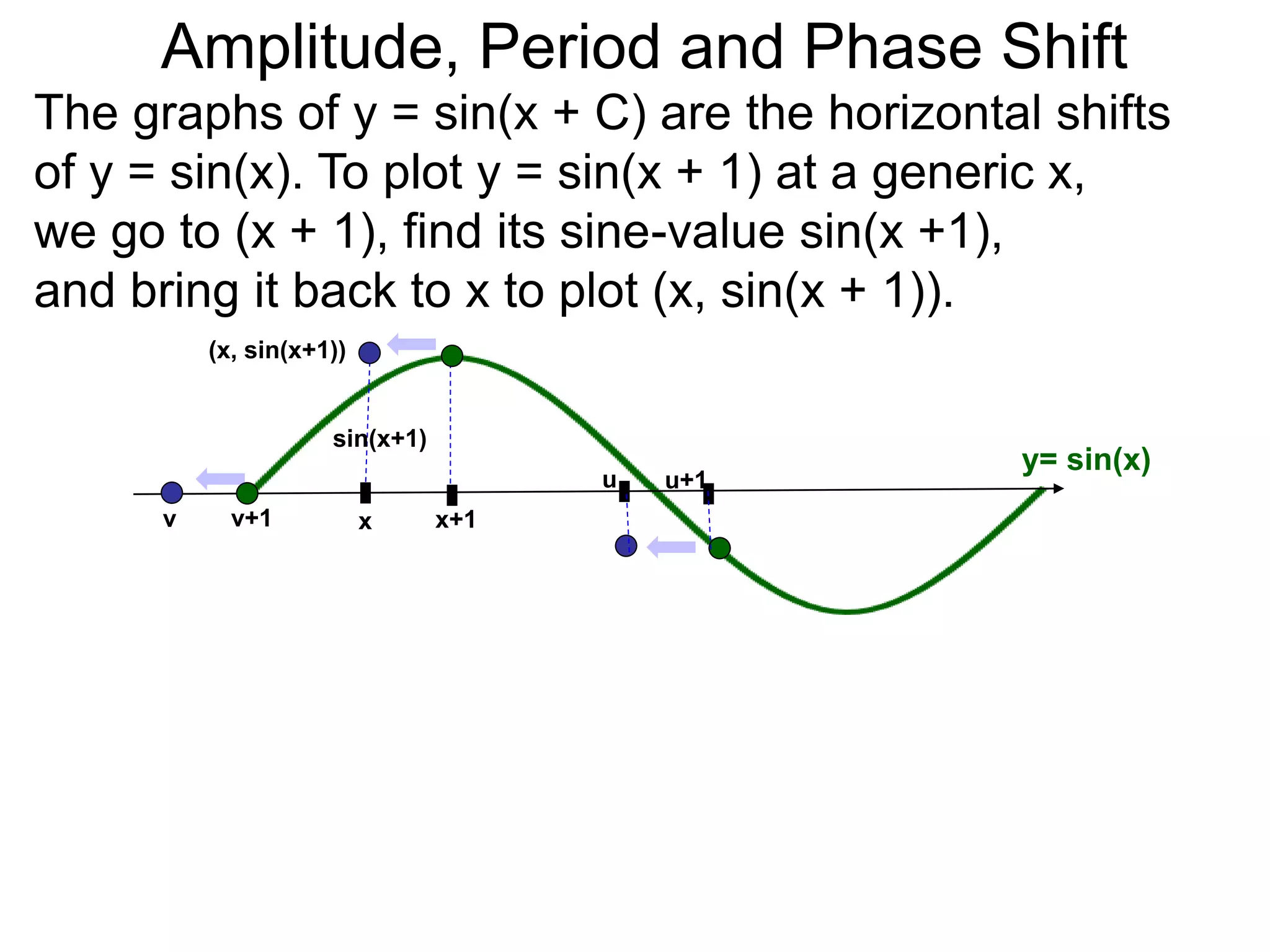
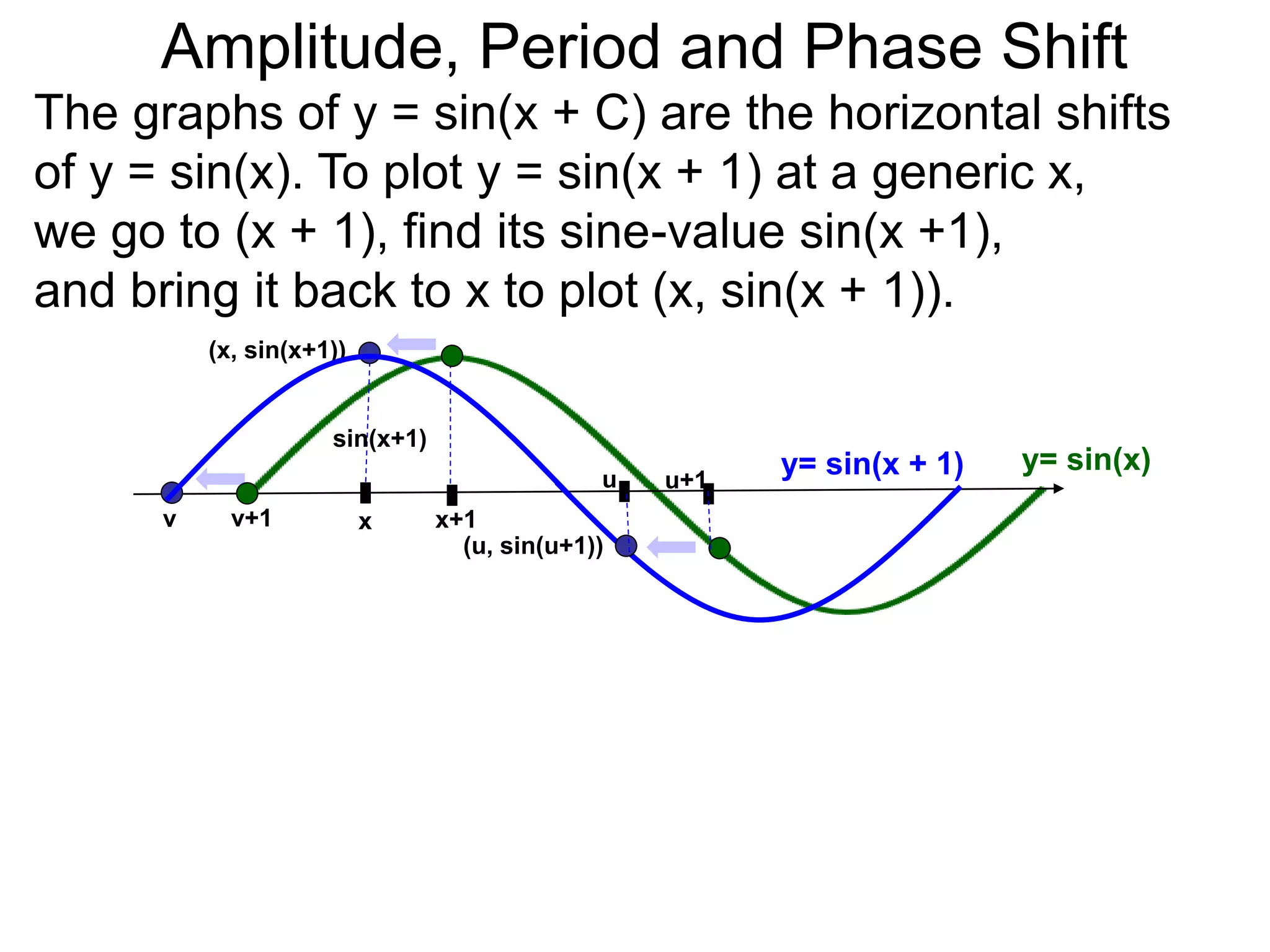
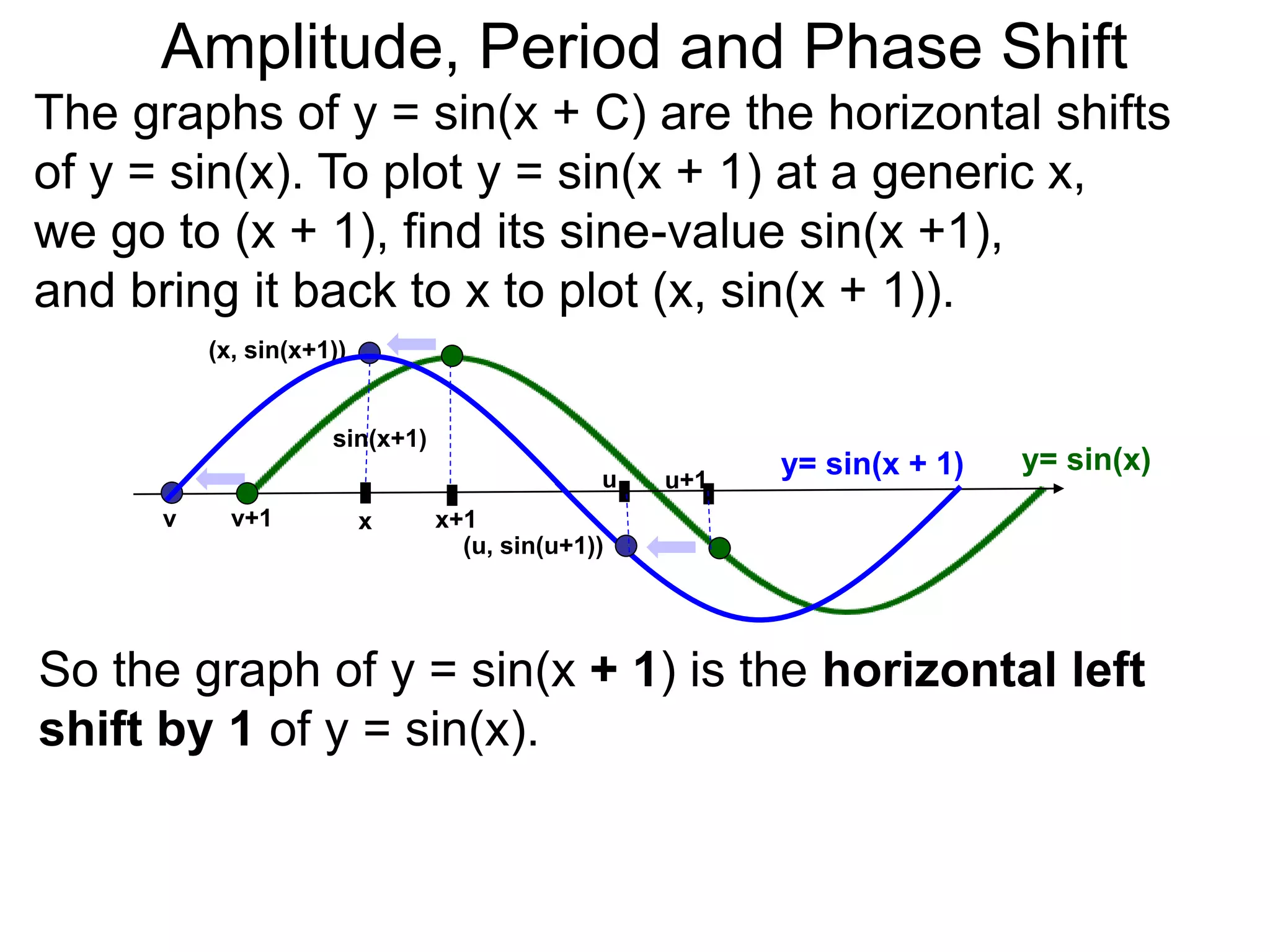
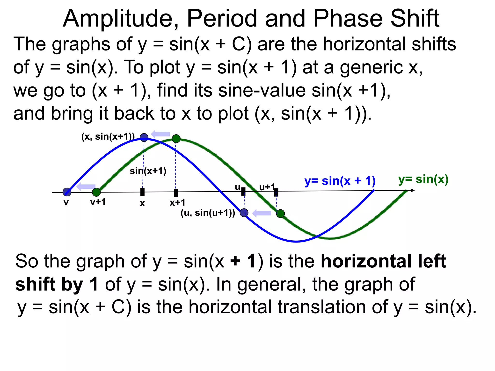
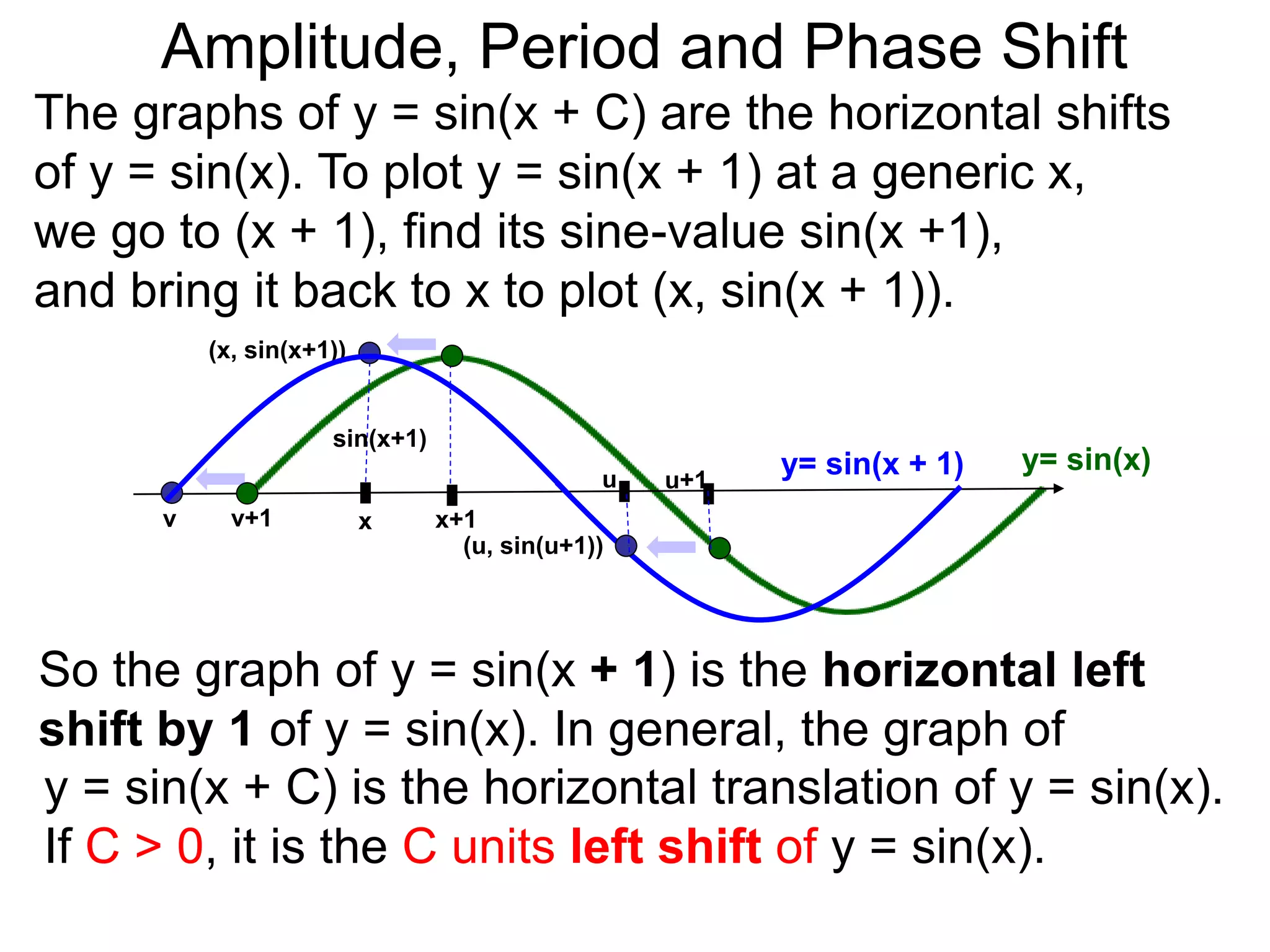
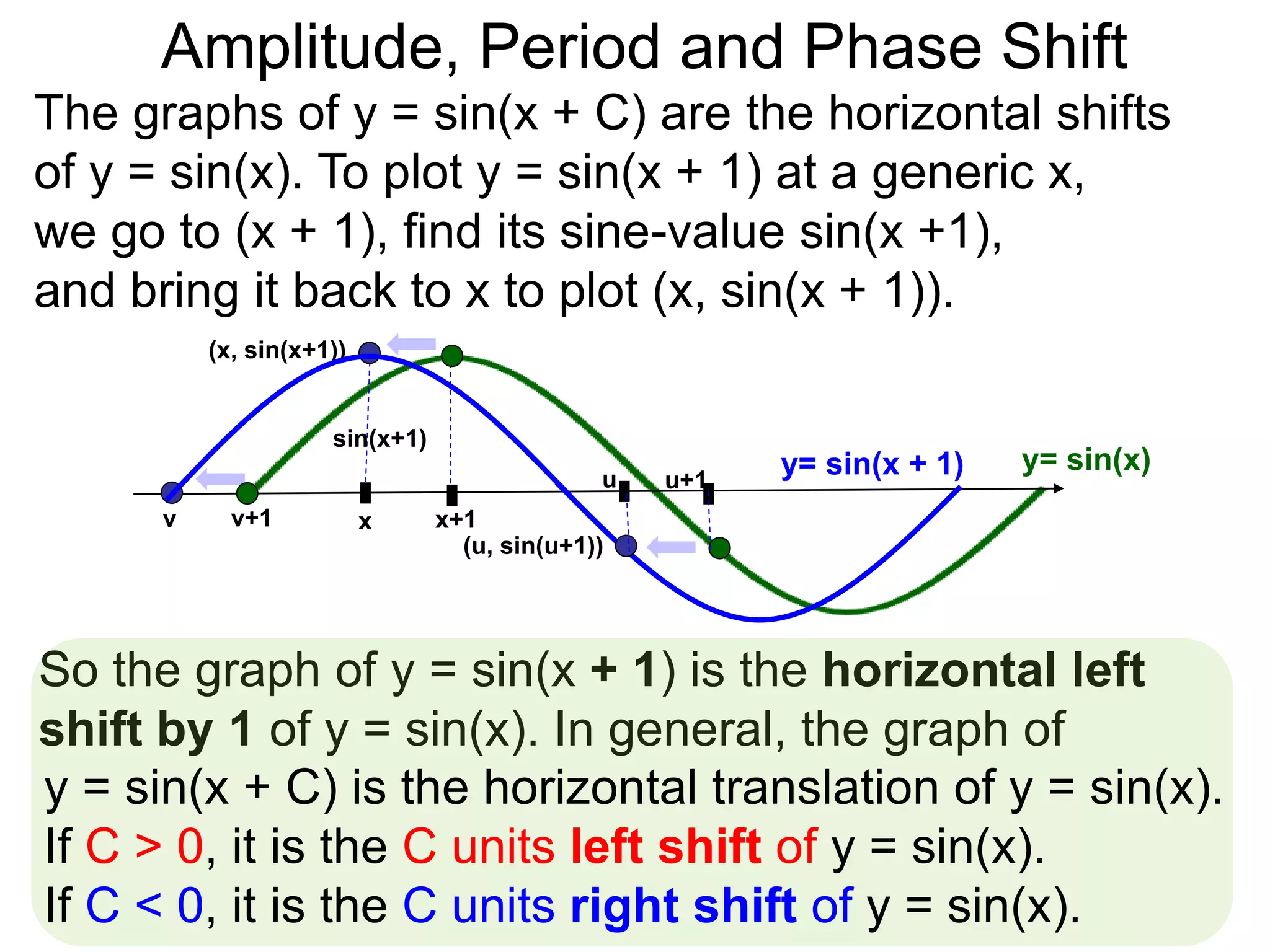
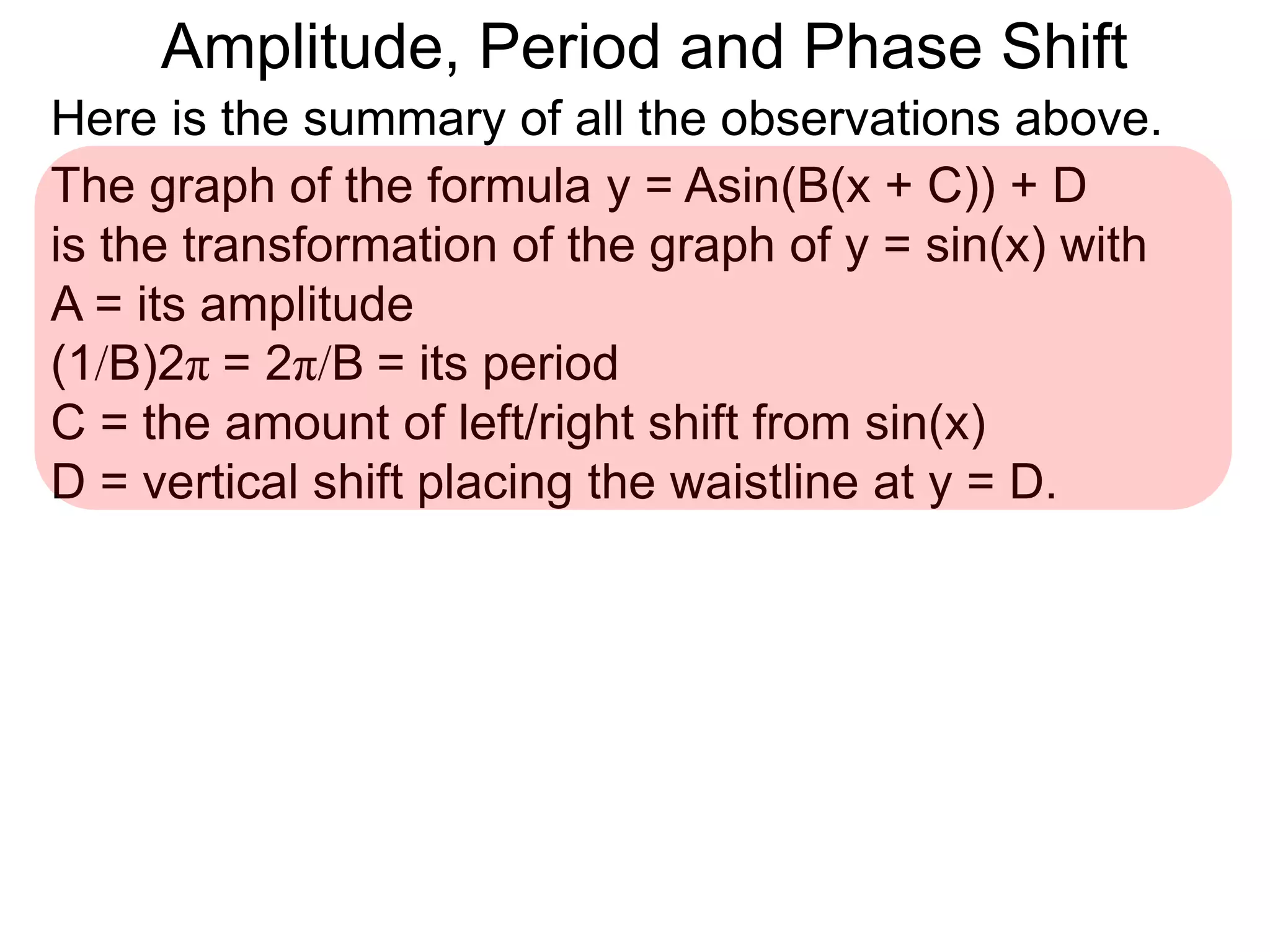
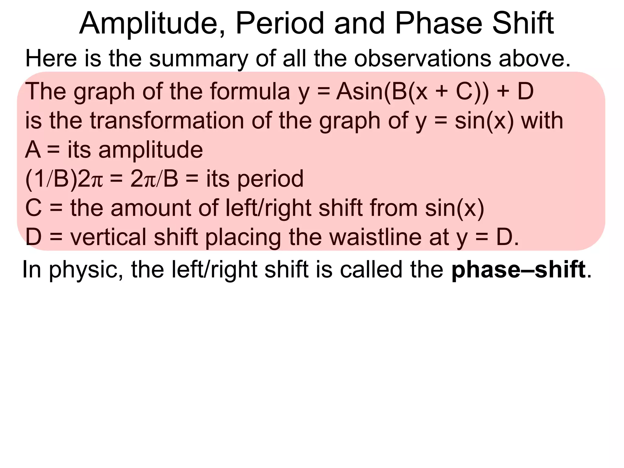
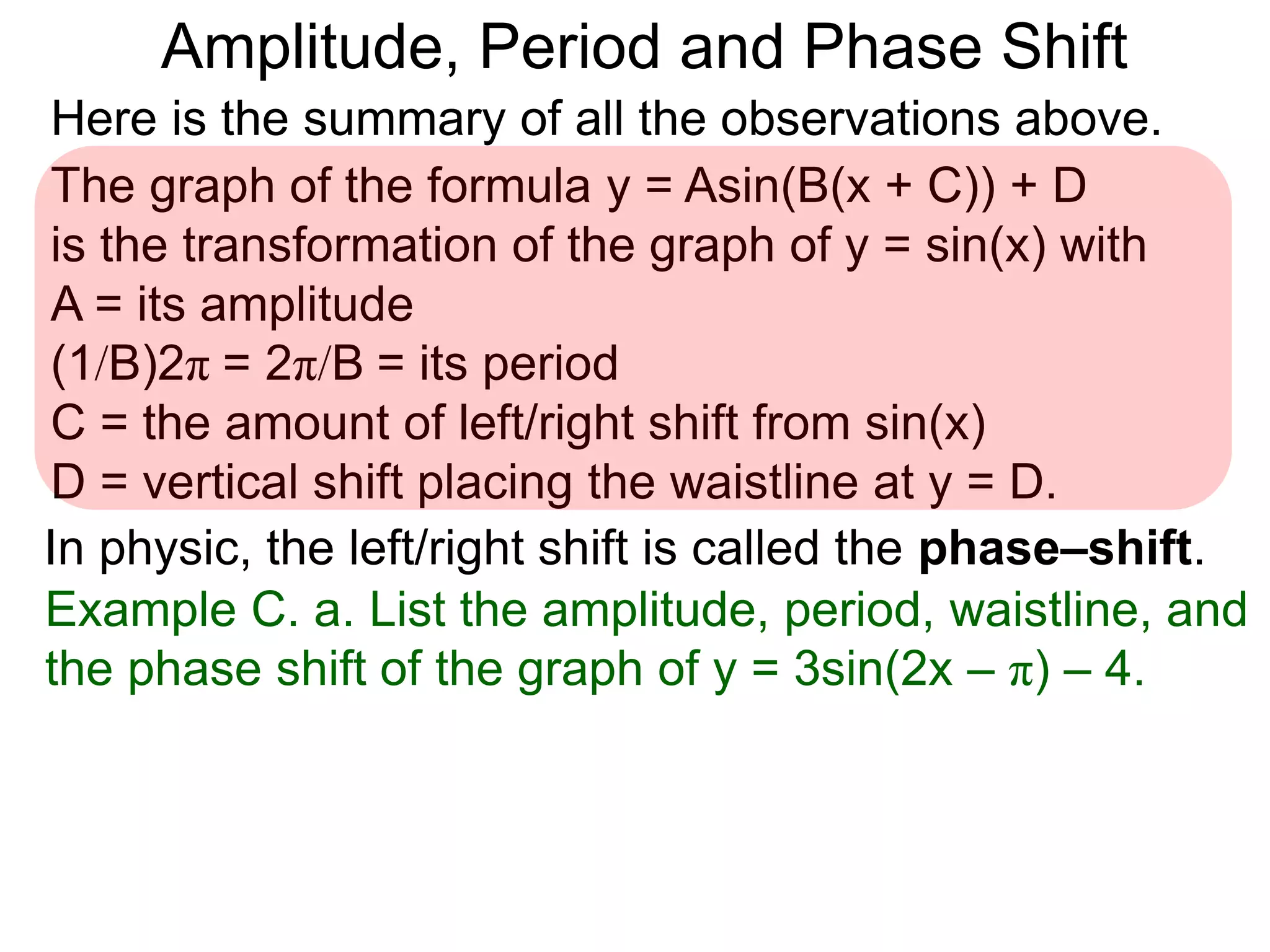
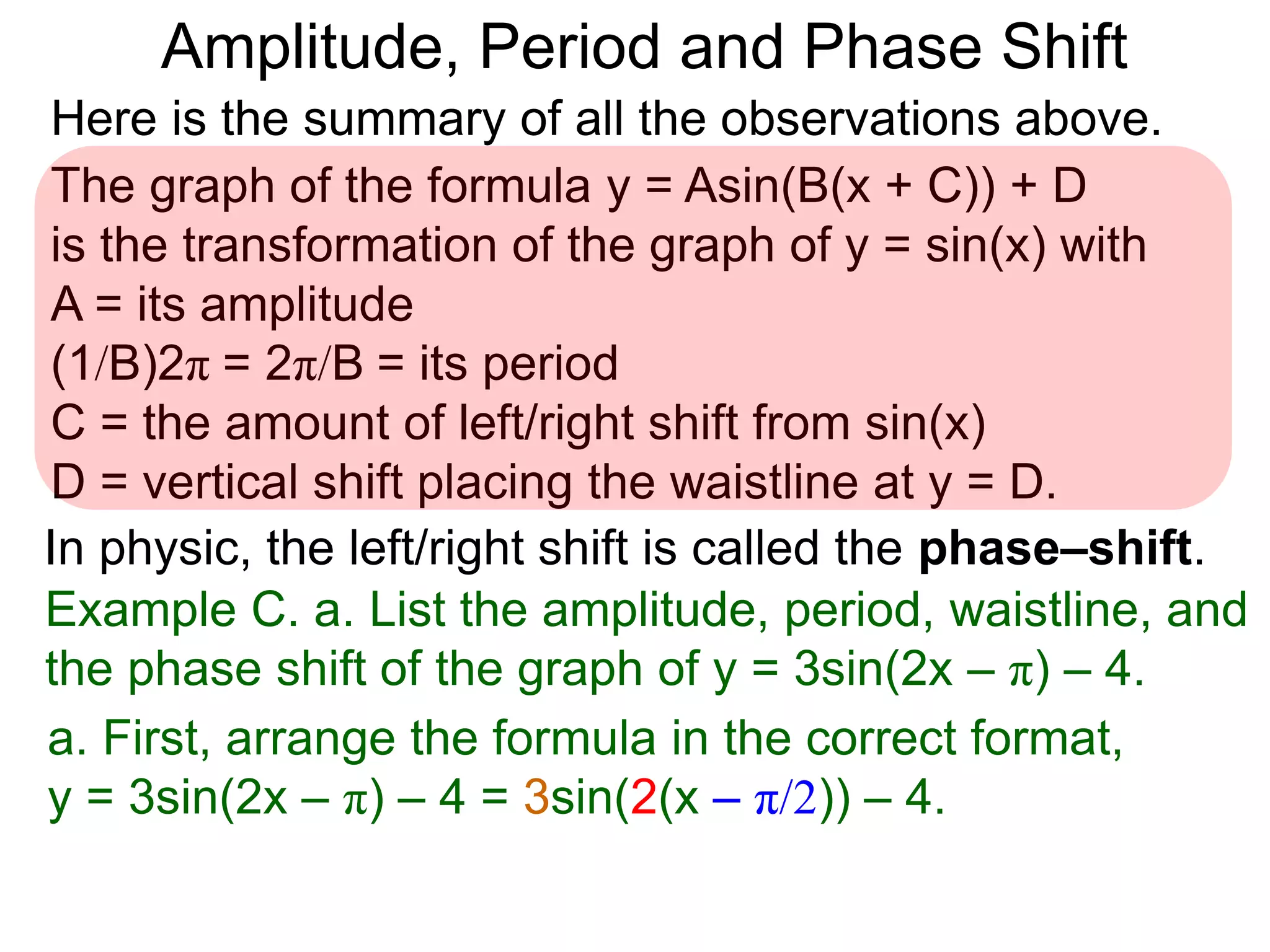
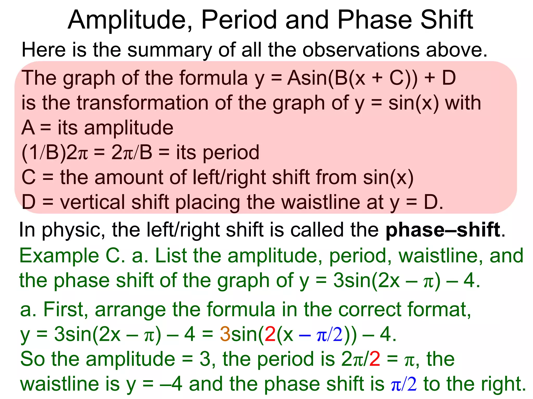
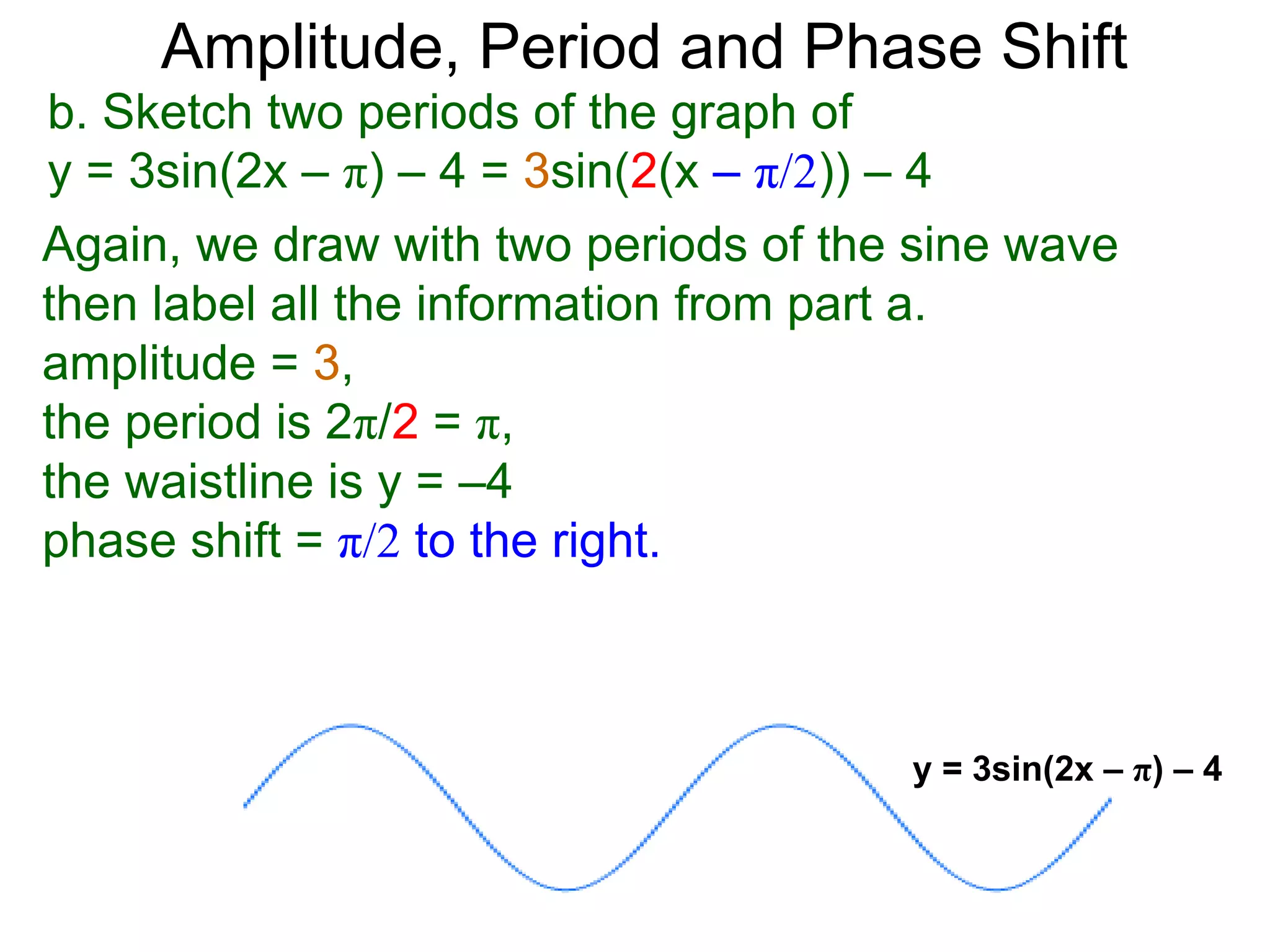
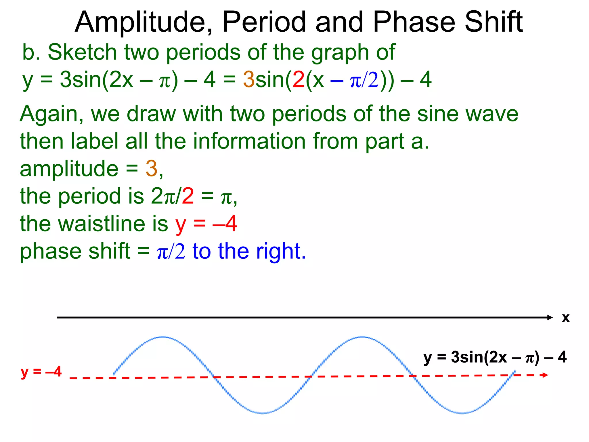
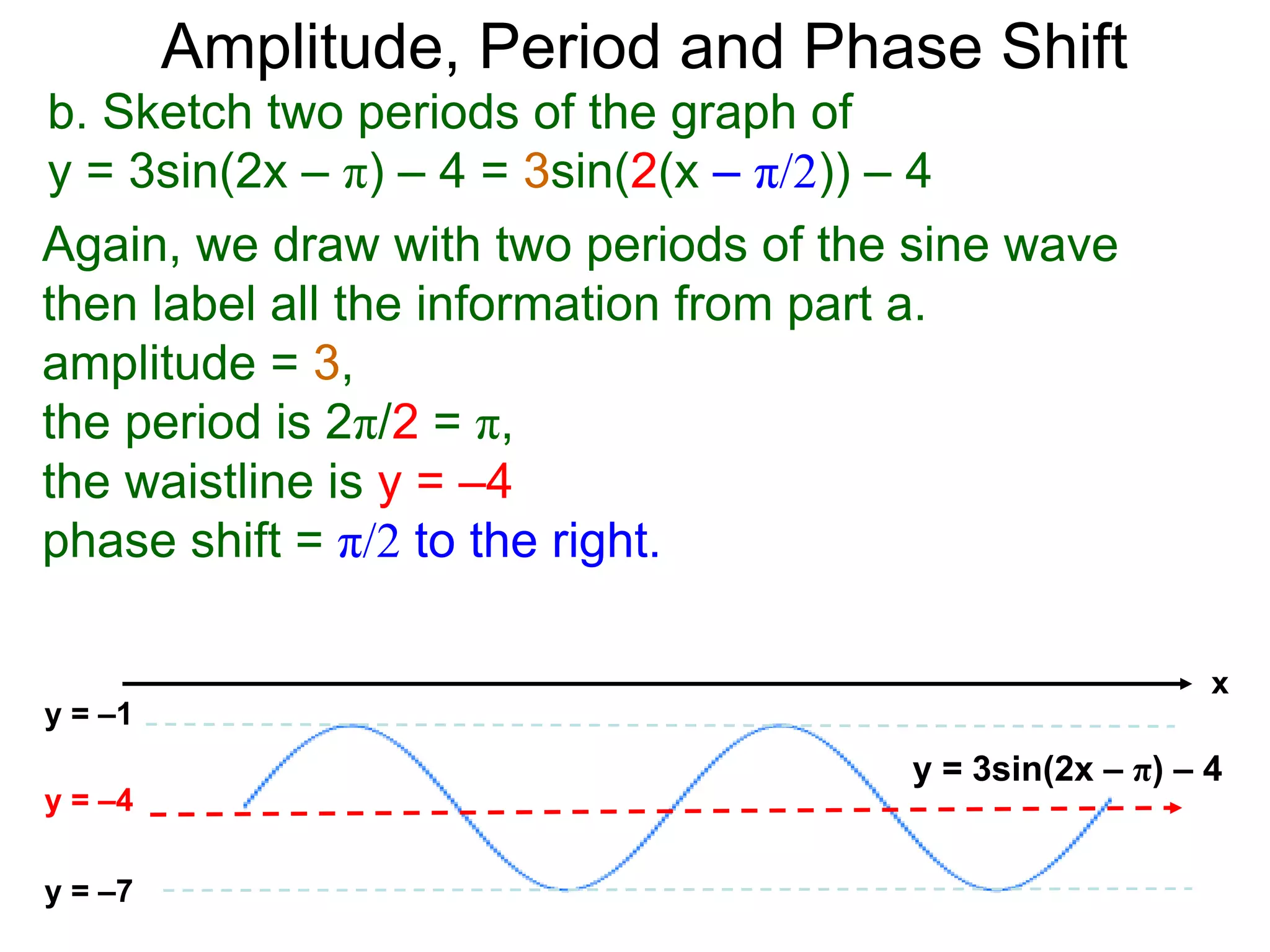
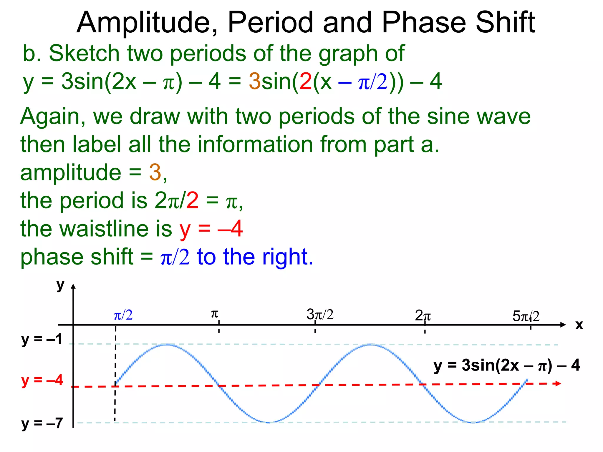
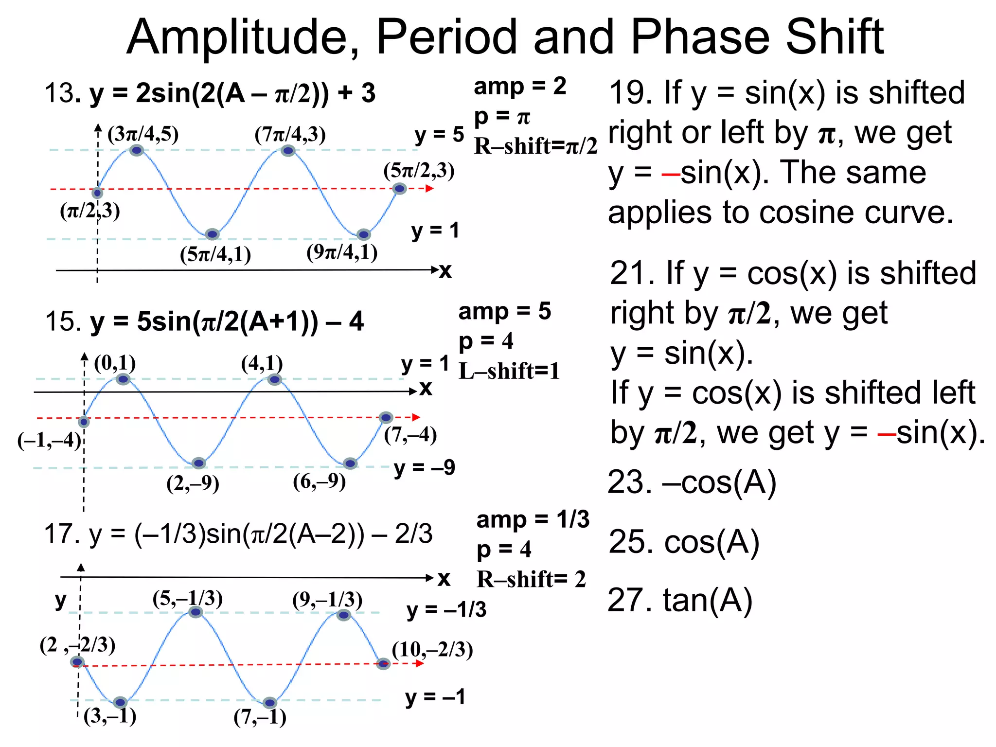
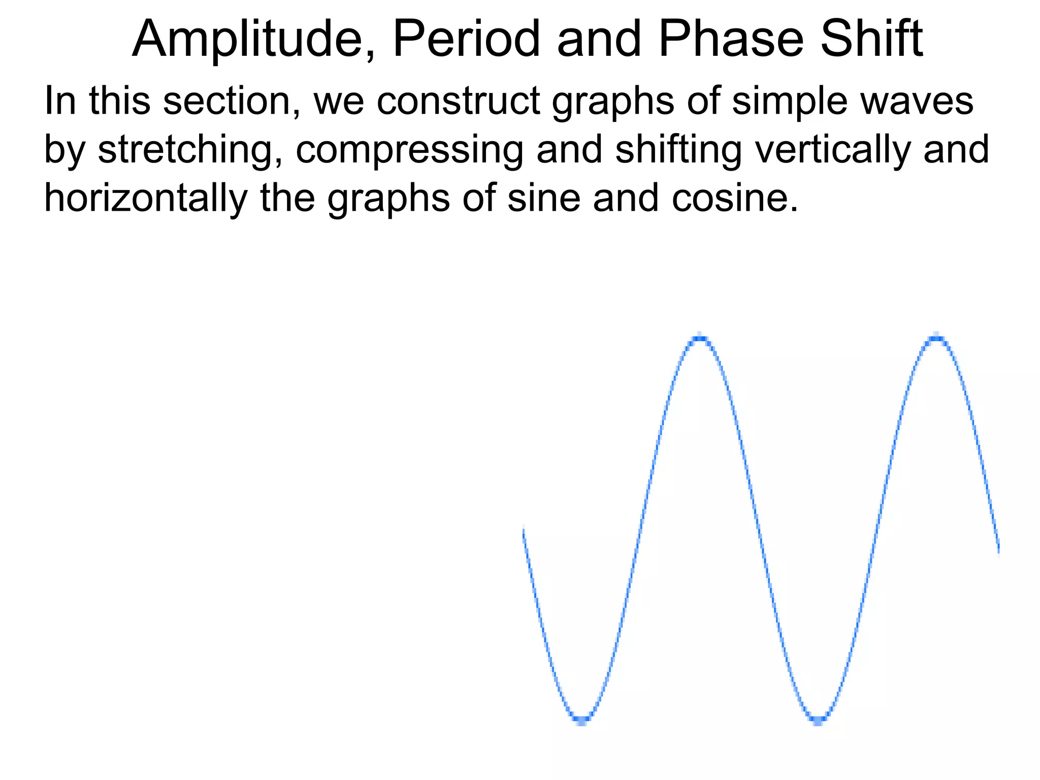
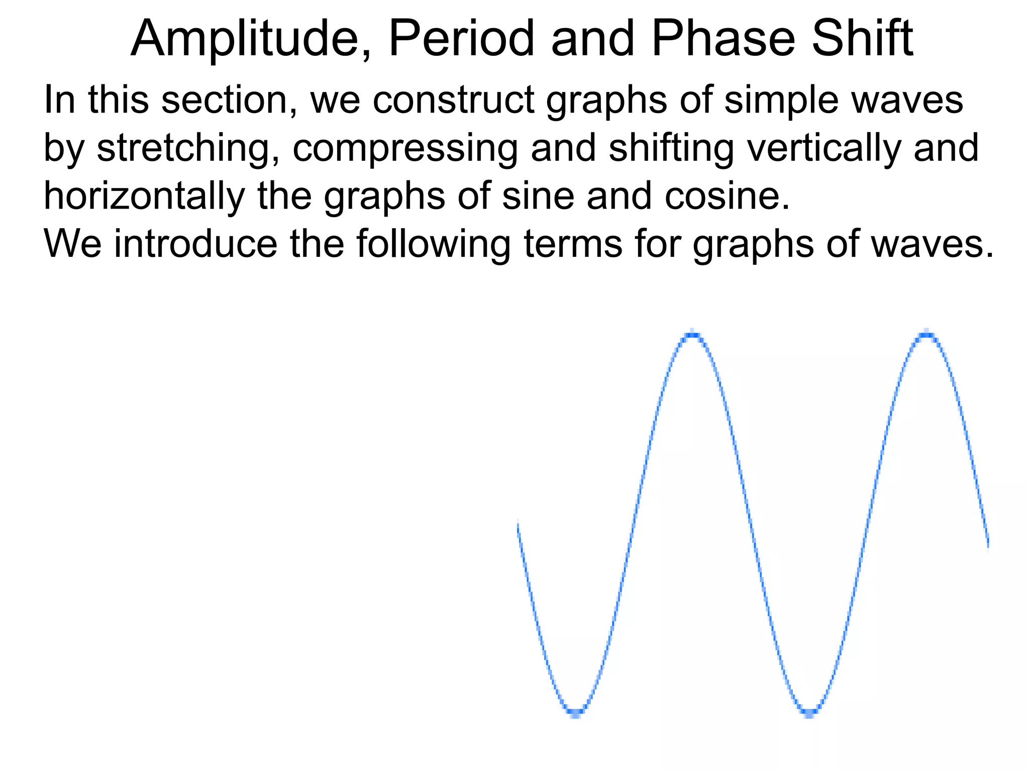
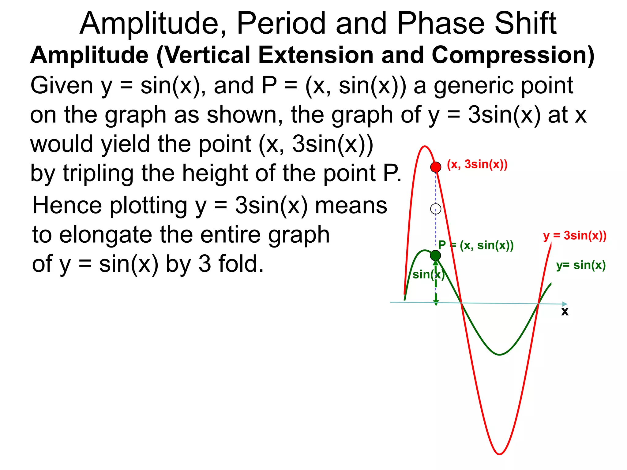
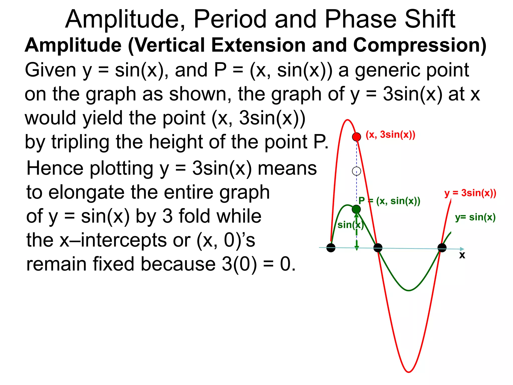
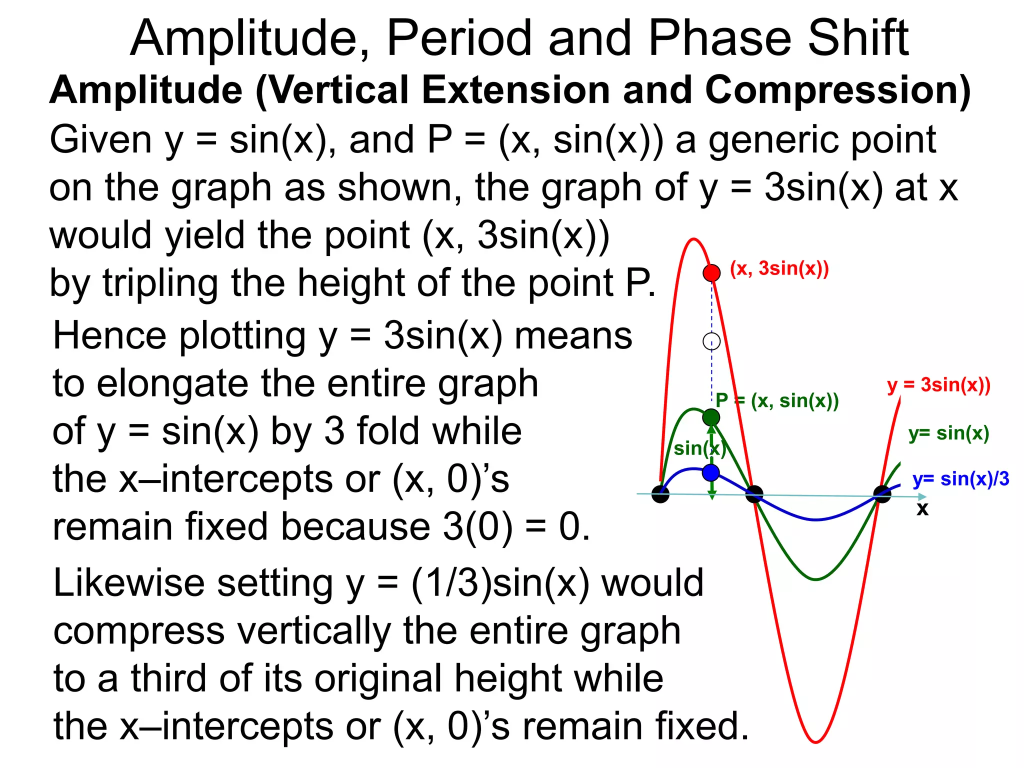
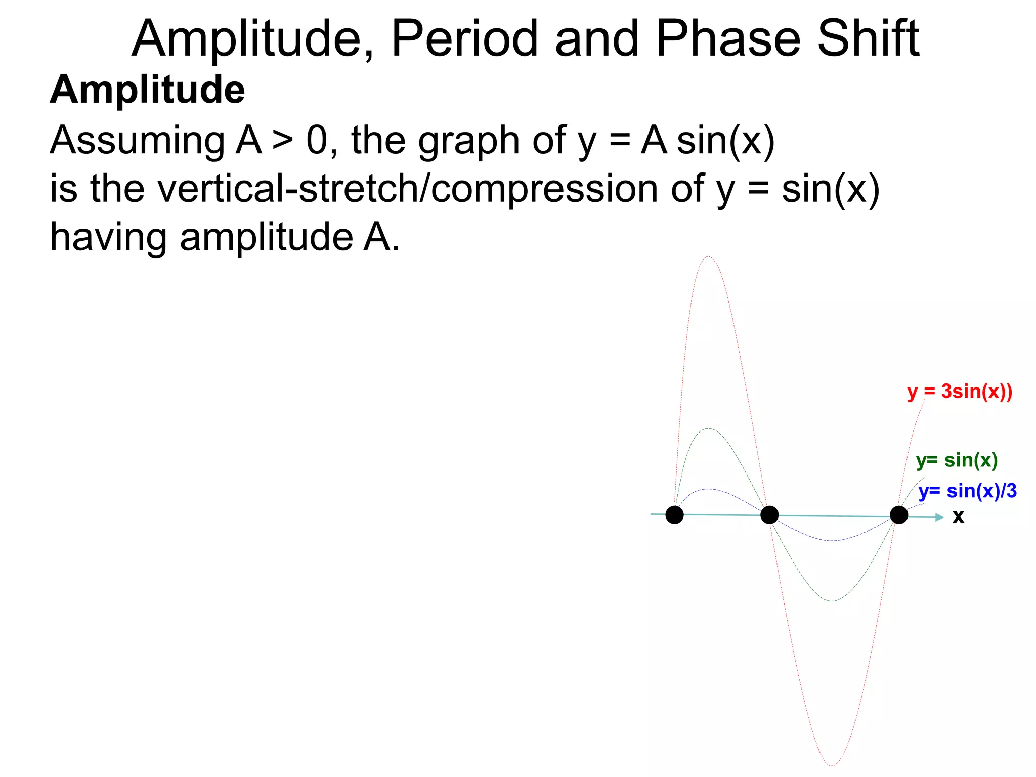
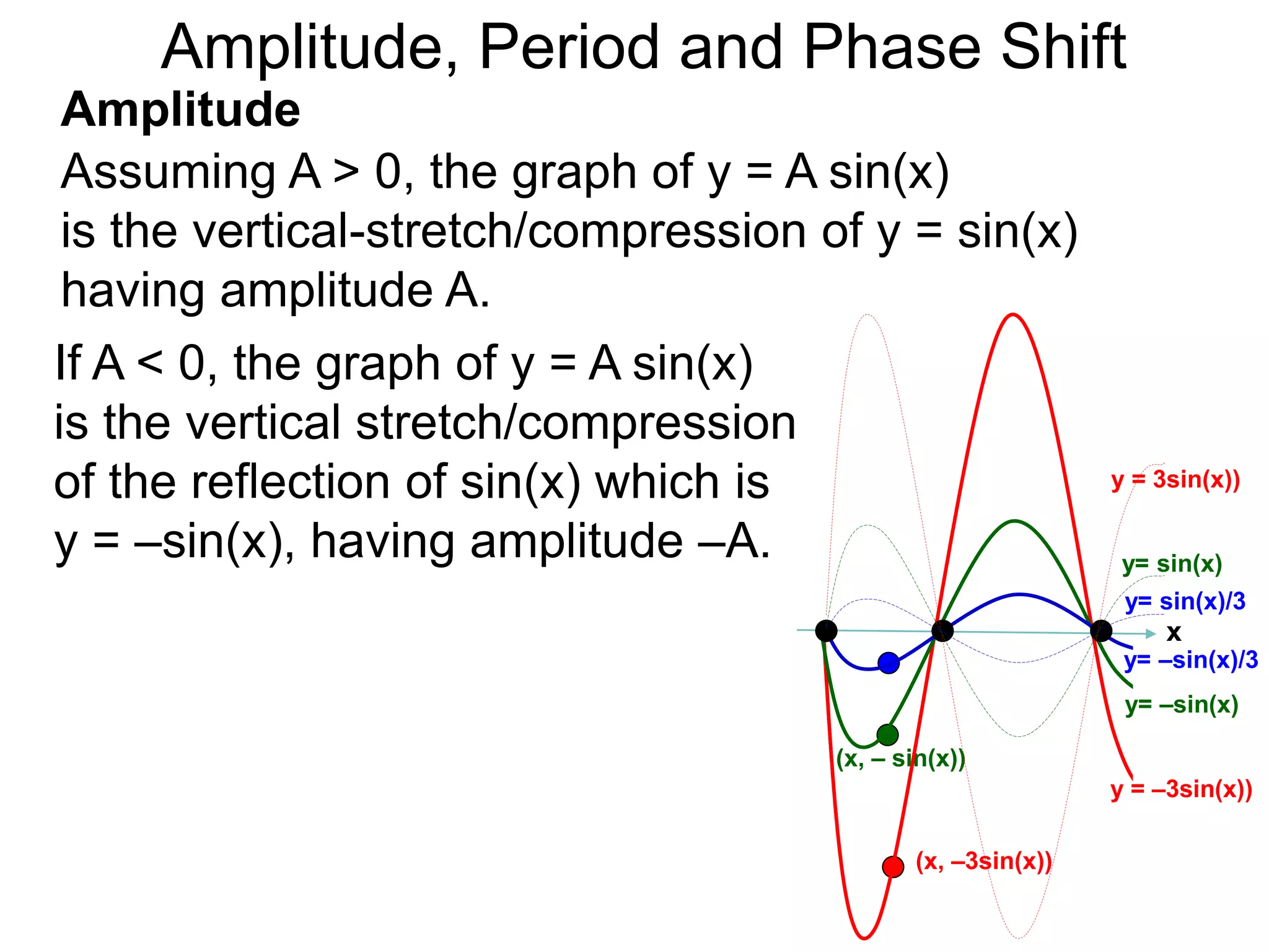
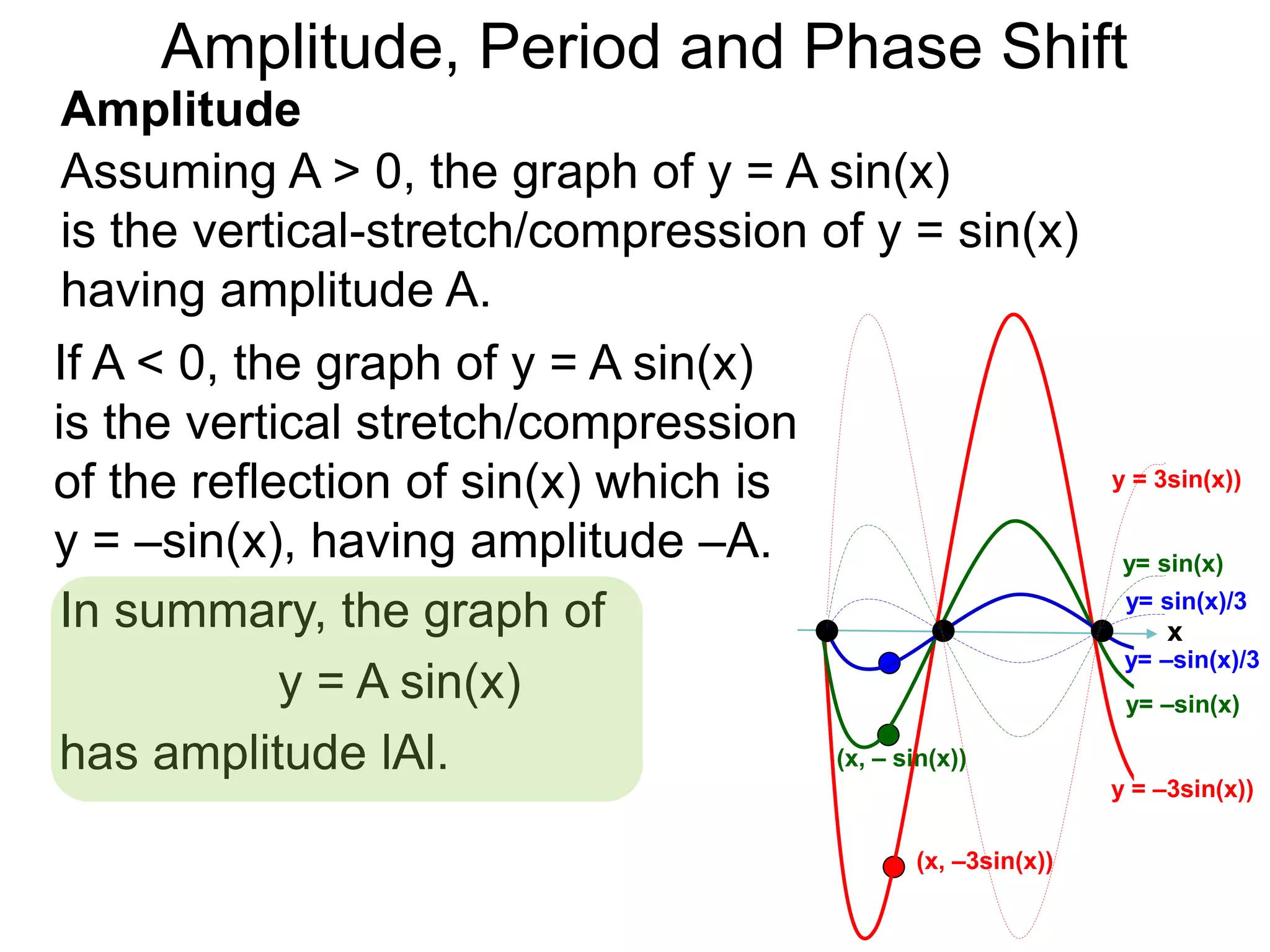
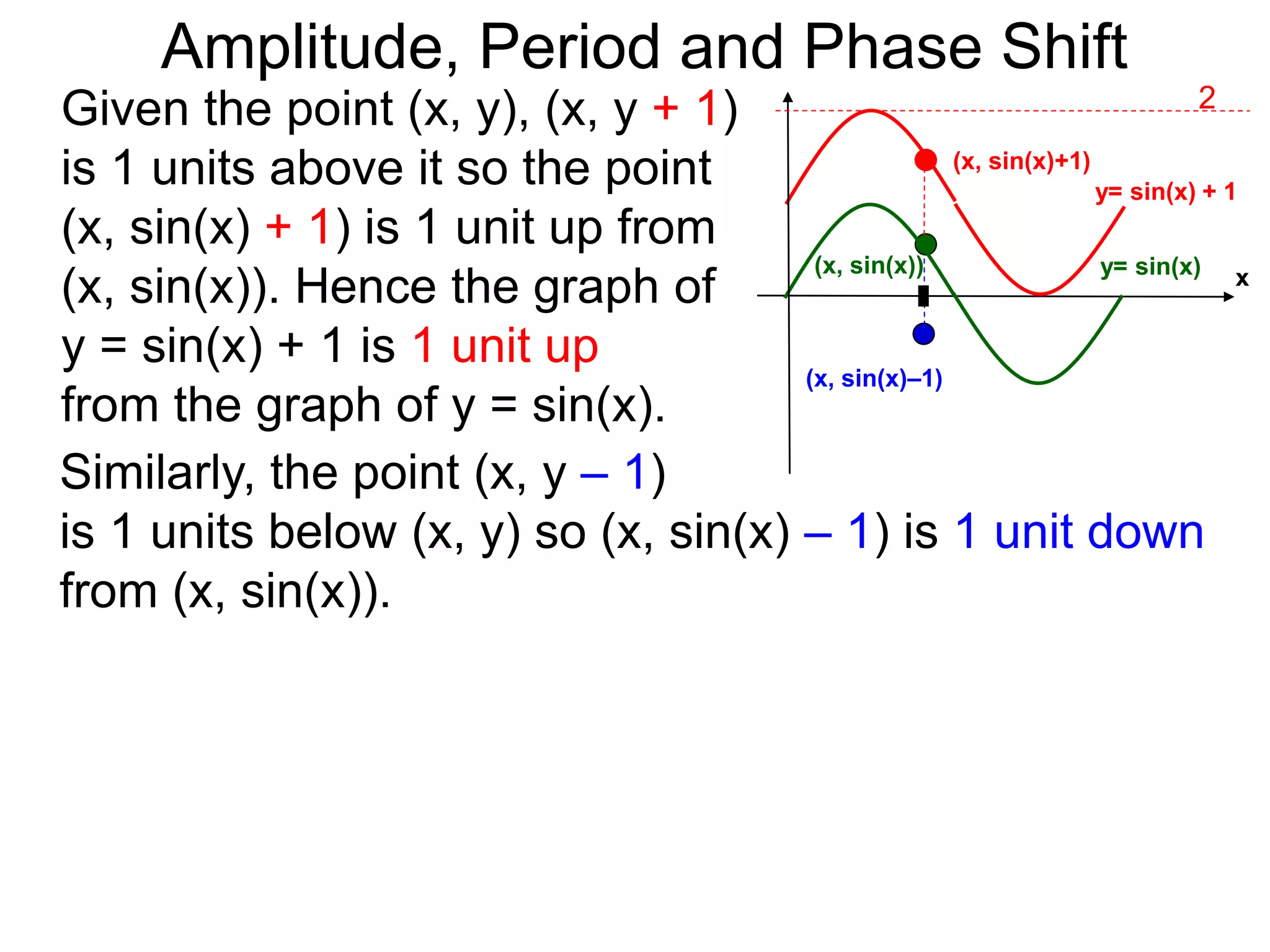
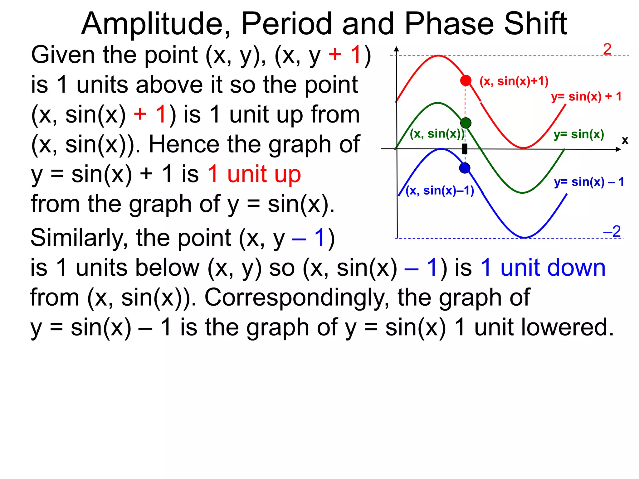
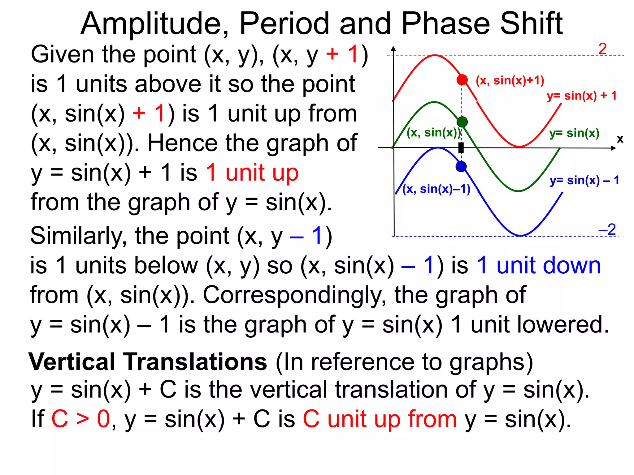
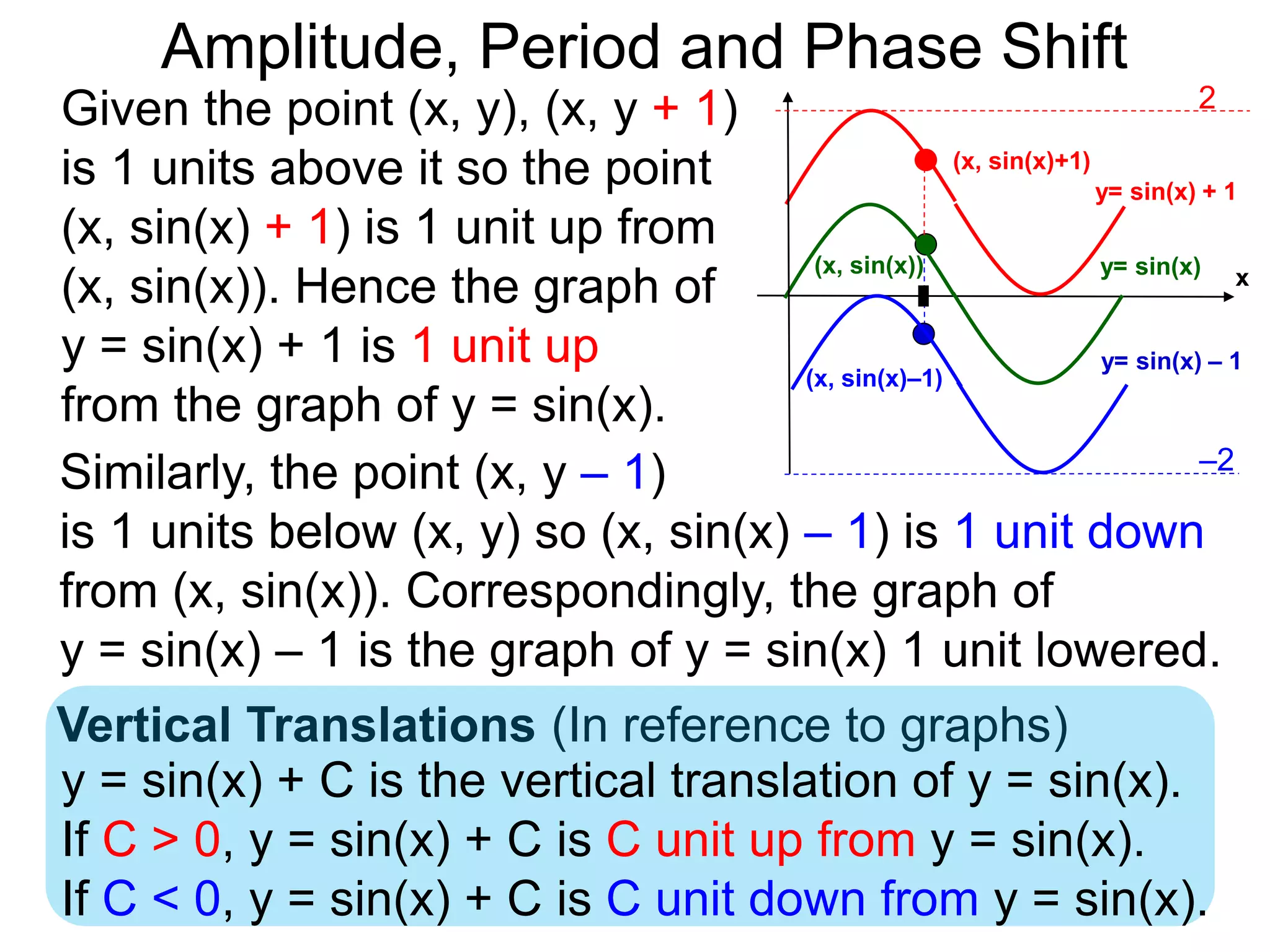
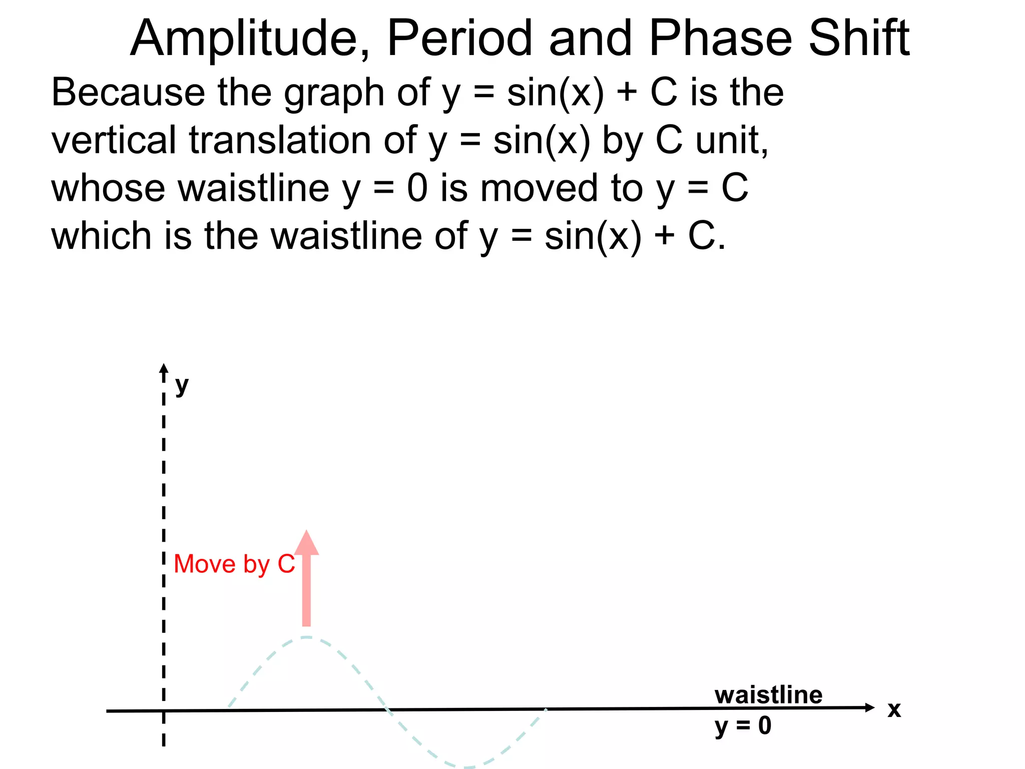
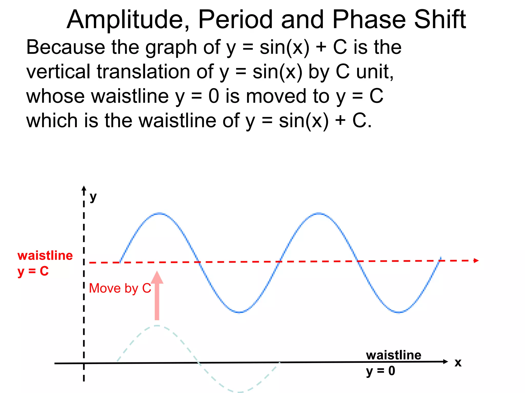
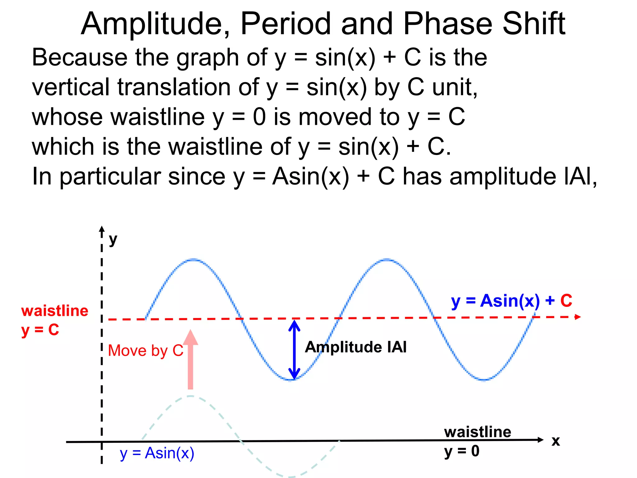
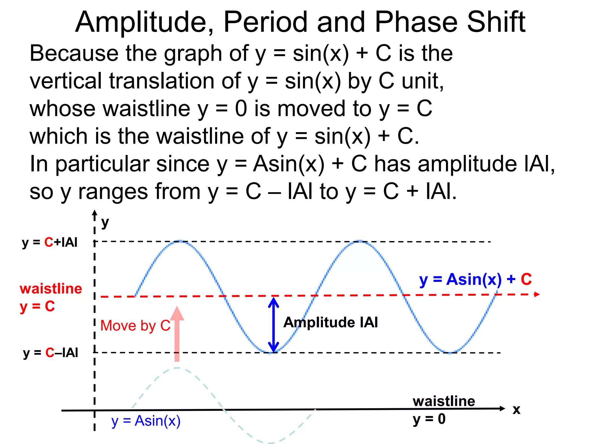
Amplitude, Period and Phase Shift
Example B.
Sketch graph of y = –3sin(x/2) + 5.
List the period and the amplitude. Draw the waistline
and the range of y.

50. The amplitude is 3 and the period is [1/(1/2)] 2π = 4π.
The waistline is y = 5, hence y ranges from 2 to 8.
Amplitude, Period and Phase Shift
Example B.
Sketch graph of y = –3sin(x/2) + 5.
List the period and the amplitude. Draw the waistline
and the range of y.

51. The amplitude is 3 and the period is [1/(1/2)] 2π = 4π.
The waistline is y = 5, hence y ranges from 2 to 8. To
sketch two periods of its graph, we start by drawing
two periods of the negative sine–wave
then label the above information as shown.
Amplitude, Period and Phase Shift
Example B.
Sketch graph of y = –3sin(x/2) + 5.
List the period and the amplitude. Draw the waistline
and the range of y.

52. The amplitude is 3 and the period is [1/(1/2)] 2π = 4π.
The waistline is y = 5, hence y ranges from 2 to 8. To
sketch two periods of its graph, we start by drawing
two periods of the negative sine–wave
then label the above information as shown.
y
Amplitude, Period and Phase Shift
Example B.
Sketch graph of y = –3sin(x/2) + 5.
List the period and the amplitude. Draw the waistline
and the range of y.

53. The amplitude is 3 and the period is [1/(1/2)] 2π = 4π.
The waistline is y = 5, hence y ranges from 2 to 8. To
sketch two periods of its graph, we start by drawing
two periods of the negative sine–wave
then label the above information as shown.
y = –3sin(x/2) + 5
y
y = 5
Amplitude, Period and Phase Shift
Example B.
Sketch graph of y = –3sin(x/2) + 5.
List the period and the amplitude. Draw the waistline
and the range of y.

54. The amplitude is 3 and the period is [1/(1/2)] 2π = 4π.
The waistline is y = 5, hence y ranges from 2 to 8. To
sketch two periods of its graph, we start by drawing
two periods of the negative sine–wave
then label the above information as shown.
y = –3sin(x/2) + 5
y
y = 5 Amplitude = 3
Amplitude, Period and Phase Shift
Example B.
Sketch graph of y = –3sin(x/2) + 5.
List the period and the amplitude. Draw the waistline
and the range of y.

55. The amplitude is 3 and the period is [1/(1/2)] 2π = 4π.
The waistline is y = 5, hence y ranges from 2 to 8. To
sketch two periods of its graph, we start by drawing
two periods of the negative sine–wave
then label the above information as shown.
2π 4π 6π 8π
y = –3sin(x/2) + 5
y
y = 5 Amplitude = 3
Amplitude, Period and Phase Shift
Example B.
Sketch graph of y = –3sin(x/2) + 5.
List the period and the amplitude. Draw the waistline
and the range of y.

56. Example B.
Sketch graph of y = –3sin(x/2) + 5.
List the period and the amplitude. Draw the waistline
and the range of y.
The amplitude is 3 and the period is [1/(1/2)] 2π = 4π.
The waistline is y = 5, hence y ranges from 2 to 8. To
sketch two periods of its graph, we start by drawing
two periods of the negative sine–wave
then label the above information as shown.
y = 5
y = 8
y = 2
2π 4π 6π 8π
y = –3sin(x/2) + 5
y
Amplitude = 3
Amplitude, Period and Phase Shift

57. The graphs of y = sin(x + C) are the horizontal shifts
of y = sin(x).
Amplitude, Period and Phase Shift

58. The graphs of y = sin(x + C) are the horizontal shifts
of y = sin(x). To plot y = sin(x + 1) at a generic x,
xx
Amplitude, Period and Phase Shift

59. The graphs of y = sin(x + C) are the horizontal shifts
of y = sin(x). To plot y = sin(x + 1) at a generic x,
we go to (x + 1),
x x+1x
Amplitude, Period and Phase Shift

60. The graphs of y = sin(x + C) are the horizontal shifts
of y = sin(x). To plot y = sin(x + 1) at a generic x,
we go to (x + 1), find its sine-value sin(x +1),
and bring it back to x to plot (x, sin(x + 1)).
x x+1
sin(x+1)
y= sin(x)
x
Amplitude, Period and Phase Shift

61. The graphs of y = sin(x + C) are the horizontal shifts
of y = sin(x). To plot y = sin(x + 1) at a generic x,
we go to (x + 1), find its sine-value sin(x +1),
and bring it back to x to plot (x, sin(x + 1)).
x x+1
sin(x+1)
(x, sin(x+1))
y= sin(x)
x
Amplitude, Period and Phase Shift

62. The graphs of y = sin(x + C) are the horizontal shifts
of y = sin(x). To plot y = sin(x + 1) at a generic x,
we go to (x + 1), find its sine-value sin(x +1),
and bring it back to x to plot (x, sin(x + 1)).
x x+1
sin(x+1)
(x, sin(x+1))
y= sin(x)
x
u
Amplitude, Period and Phase Shift

63. The graphs of y = sin(x + C) are the horizontal shifts
of y = sin(x). To plot y = sin(x + 1) at a generic x,
we go to (x + 1), find its sine-value sin(x +1),
and bring it back to x to plot (x, sin(x + 1)).
x x+1
sin(x+1)
(x, sin(x+1))
y= sin(x)
x
u u+1
Amplitude, Period and Phase Shift

64. The graphs of y = sin(x + C) are the horizontal shifts
of y = sin(x). To plot y = sin(x + 1) at a generic x,
we go to (x + 1), find its sine-value sin(x +1),
and bring it back to x to plot (x, sin(x + 1)).
x x+1
sin(x+1)
(x, sin(x+1))
y= sin(x)
x
u u+1
v
Amplitude, Period and Phase Shift

65. The graphs of y = sin(x + C) are the horizontal shifts
of y = sin(x). To plot y = sin(x + 1) at a generic x,
we go to (x + 1), find its sine-value sin(x +1),
and bring it back to x to plot (x, sin(x + 1)).
x x+1
sin(x+1)
(x, sin(x+1))
y= sin(x)
x
u u+1
v v+1
Amplitude, Period and Phase Shift

66. The graphs of y = sin(x + C) are the horizontal shifts
of y = sin(x). To plot y = sin(x + 1) at a generic x,
we go to (x + 1), find its sine-value sin(x +1),
and bring it back to x to plot (x, sin(x + 1)).
x x+1
sin(x+1)
v v+1
(x, sin(x+1))
y= sin(x)y= sin(x + 1)u u+1
(u, sin(u+1))
x
Amplitude, Period and Phase Shift

67. The graphs of y = sin(x + C) are the horizontal shifts
of y = sin(x). To plot y = sin(x + 1) at a generic x,
we go to (x + 1), find its sine-value sin(x +1),
and bring it back to x to plot (x, sin(x + 1)).
x x+1
sin(x+1)
v v+1
(x, sin(x+1))
y= sin(x)y= sin(x + 1)u u+1
So the graph of y = sin(x + 1) is the horizontal left
shift by 1 of y = sin(x).
(u, sin(u+1))
x
Amplitude, Period and Phase Shift

68. The graphs of y = sin(x + C) are the horizontal shifts
of y = sin(x). To plot y = sin(x + 1) at a generic x,
we go to (x + 1), find its sine-value sin(x +1),
and bring it back to x to plot (x, sin(x + 1)).
x x+1
sin(x+1)
v v+1
(x, sin(x+1))
y= sin(x)y= sin(x + 1)u u+1
So the graph of y = sin(x + 1) is the horizontal left
shift by 1 of y = sin(x). In general, the graph of
(u, sin(u+1))
y = sin(x + C) is the horizontal translation of y = sin(x).
x
Amplitude, Period and Phase Shift

69. The graphs of y = sin(x + C) are the horizontal shifts
of y = sin(x). To plot y = sin(x + 1) at a generic x,
we go to (x + 1), find its sine-value sin(x +1),
and bring it back to x to plot (x, sin(x + 1)).
x x+1
sin(x+1)
v v+1
(x, sin(x+1))
y= sin(x)y= sin(x + 1)u u+1
So the graph of y = sin(x + 1) is the horizontal left
shift by 1 of y = sin(x). In general, the graph of
(u, sin(u+1))
y = sin(x + C) is the horizontal translation of y = sin(x).
If C > 0, it is the C units left shift of y = sin(x).
x
Amplitude, Period and Phase Shift

70. The graphs of y = sin(x + C) are the horizontal shifts
of y = sin(x). To plot y = sin(x + 1) at a generic x,
we go to (x + 1), find its sine-value sin(x +1),
and bring it back to x to plot (x, sin(x + 1)).
x x+1
sin(x+1)
v v+1
(x, sin(x+1))
y= sin(x)y= sin(x + 1)u u+1
So the graph of y = sin(x + 1) is the horizontal left
shift by 1 of y = sin(x). In general, the graph of
(u, sin(u+1))
y = sin(x + C) is the horizontal translation of y = sin(x).
If C > 0, it is the C units left shift of y = sin(x).
If C < 0, it is the C units right shift of y = sin(x).
x
Amplitude, Period and Phase Shift

71. Here is the summary of all the observations above.
The graph of the formula y = Asin(B(x + C)) + D
is the transformation of the graph of y = sin(x) with
A = its amplitude
(1/B)2π = 2π/B = its period
C = the amount of left/right shift from sin(x)
D = vertical shift placing the waistline at y = D.
Amplitude, Period and Phase Shift

72. Here is the summary of all the observations above.
The graph of the formula y = Asin(B(x + C)) + D
is the transformation of the graph of y = sin(x) with
A = its amplitude
(1/B)2π = 2π/B = its period
C = the amount of left/right shift from sin(x)
D = vertical shift placing the waistline at y = D.
In physic, the left/right shift is called the phase–shift.
Amplitude, Period and Phase Shift

73. Here is the summary of all the observations above.
Example C. a. List the amplitude, period, waistline, and
the phase shift of the graph of y = 3sin(2x – π) – 4.
The graph of the formula y = Asin(B(x + C)) + D
is the transformation of the graph of y = sin(x) with
A = its amplitude
(1/B)2π = 2π/B = its period
C = the amount of left/right shift from sin(x)
D = vertical shift placing the waistline at y = D.
In physic, the left/right shift is called the phase–shift.
Amplitude, Period and Phase Shift

74. Here is the summary of all the observations above.
Example C. a. List the amplitude, period, waistline, and
the phase shift of the graph of y = 3sin(2x – π) – 4.
The graph of the formula y = Asin(B(x + C)) + D
is the transformation of the graph of y = sin(x) with
A = its amplitude
(1/B)2π = 2π/B = its period
C = the amount of left/right shift from sin(x)
D = vertical shift placing the waistline at y = D.
In physic, the left/right shift is called the phase–shift.
a. First, arrange the formula in the correct format,
y = 3sin(2x – π) – 4 = 3sin(2(x – π/2)) – 4.
Amplitude, Period and Phase Shift

75. Here is the summary of all the observations above.
Example C. a. List the amplitude, period, waistline, and
the phase shift of the graph of y = 3sin(2x – π) – 4.
The graph of the formula y = Asin(B(x + C)) + D
is the transformation of the graph of y = sin(x) with
A = its amplitude
(1/B)2π = 2π/B = its period
C = the amount of left/right shift from sin(x)
D = vertical shift placing the waistline at y = D.
In physic, the left/right shift is called the phase–shift.
a. First, arrange the formula in the correct format,
y = 3sin(2x – π) – 4 = 3sin(2(x – π/2)) – 4.
So the amplitude = 3, the period is 2π/2 = π, the
waistline is y = –4 and the phase shift is π/2 to the right.
Amplitude, Period and Phase Shift

76. b. Sketch two periods of the graph of
y = 3sin(2x – π) – 4 = 3sin(2(x – π/2)) – 4
Amplitude, Period and Phase Shift

77. b. Sketch two periods of the graph of
y = 3sin(2x – π) – 4 = 3sin(2(x – π/2)) – 4
Again, we draw with two periods of the sine wave
then label all the information from part a.
amplitude = 3,
the period is 2π/2 = π,
the waistline is y = –4
phase shift = π/2 to the right.
Amplitude, Period and Phase Shift

78. b. Sketch two periods of the graph of
y = 3sin(2x – π) – 4 = 3sin(2(x – π/2)) – 4
Again, we draw with two periods of the sine wave
then label all the information from part a.
amplitude = 3,
the period is 2π/2 = π,
the waistline is y = –4
phase shift = π/2 to the right.
y = 3sin(2x – π) – 4
Amplitude, Period and Phase Shift

79. b. Sketch two periods of the graph of
y = 3sin(2x – π) – 4 = 3sin(2(x – π/2)) – 4
Again, we draw with two periods of the sine wave
then label all the information from part a.
amplitude = 3,
the period is 2π/2 = π,
the waistline is y = –4
phase shift = π/2 to the right.
y = –4
y = 3sin(2x – π) – 4
x
Amplitude, Period and Phase Shift

80. b. Sketch two periods of the graph of
y = 3sin(2x – π) – 4 = 3sin(2(x – π/2)) – 4
Again, we draw with two periods of the sine wave
then label all the information from part a.
amplitude = 3,
the period is 2π/2 = π,
the waistline is y = –4
phase shift = π/2 to the right.
y = –4
y = –1
y = –7
y = 3sin(2x – π) – 4
x
Amplitude, Period and Phase Shift

81. b. Sketch two periods of the graph of
y = 3sin(2x – π) – 4 = 3sin(2(x – π/2)) – 4
Again, we draw with two periods of the sine wave
then label all the information from part a.
amplitude = 3,
the period is 2π/2 = π,
the waistline is y = –4
phase shift = π/2 to the right.
y = –4
y = –1
y = –7
π 3π/2 2π 5π/2
y = 3sin(2x – π) – 4
π/2
y
x
Amplitude, Period and Phase Shift

82. c. Label the points on the waistline, the high points,
and the low points on the graph.
y = –4
y = –1
y = –7
π 3π/2 2π 5π/2
y = 3sin(2x – π) – 4
π/2
y
x
Amplitude, Period and Phase Shift
(π/2, –4) (π,–4) (3π/2,–4) (2π,–4)
(3π/4,–1) (7π/4,–1)
Amplitude = 3,
Period is 2π/2 = π,
Waistline is y = –4
Phase Shift = π/2 to the right.
(5π/4,–7) (9π/4,–7)

83. List the amplitude, the period and draw two periods of the
following formulas. Label the high points and the low points
on the graph.
1. y = 3sin(2A)
Amplitude, Period and Phase Shift
2. y = 2sin(3A) 3. y = –3sin(2A) + 1
4. y = –2sin(3A) – 2 5. y = 5sin(A/2) – 3
6. y = –½ sin(2A) – 3/2 7. y = (–1/3)sin(2A) – 2/3
8. y = –2sin(πA) – 2 9. y = 5sin(2πA) – 3
10. y = –½ sin(2πA) – 3/2 11. y = (–1/3)sin(πA/2) – 2/3
Write the following formulas in the form of
y = Asin(B(x + C)) + D. List the amplitude, the period and draw
two periods of the following formulas. Label the points on the
waistline, the high points, and the low points on the graph.
12. y = 3sin(2A + π) – 1 13. y = 2sin(2A – π) + 3
14. y = –2sin(A/2 – π/2) – 2 15. y = 5sin(Aπ/2 + π/2) – 4
16. y = –½ sin(2πA – π) – 3/2 17. y = (–1/3)sin(Aπ/2 – π) – 2/3

84. Use the fact that cos(–A) = cos(A), sin(–A) = –sin(A),
tan(–A) = –tan(A) in terms of sin(A), cos(A) and tan(A).
22. sin(π – A) =
23. cos(π – A) =
26. tan(π – A) =
24. cos(π/2 – A) =
25. sin(π/2 – A) =
27. cot(π/2 – A) =
Interpret the following identities from section 9 in terms
of shifts of their graphs.
19. sin(A ± π) = –sin(A), cos(A ± π) = –cos(A)
20. sin(A + π/2) = cos(A), sin(A – π/2) = –cos(A)
21. cos(A – π/2) = sin(A), cos(A + π/2) = –sin(A)
Amplitude, Period and Phase Shift

85. y = 3
π
y
Amplitude, Period and Phase Shift
1. y = 3sin(2A)
π/2
3π/2 2π
y = –3
(3π/4,–3)
(π/4,3) ( 5π/4,3)
(7π/4,–3)
y = 4y
3. y = –3sin(2A) + 1
y = –2
(π/4,–2)
( 0,1)
(3π/4,4)
(5π/4,–2)
(7π/4,4)
amp = 3 p = π amp = 3 p = π
(2π,1)
5. y = 5sin(A/2) – 3
y = 2y
y = –8
(3π,–8)
(π,2) ( 5π,2)
(7π,–8)
amp = 5 p = 4π
( 0,–3)
(8π,–3)
7. y = (–1/3)sin(2A) – 2/3
y = –1/3y
y = –1
(π/4,–1)
( 0,–2/3)
(3π/4,–1/3)
(5π/4,–1)
(7π/4,–1/3)
amp = 1/3
p = π
(2π,–2/3)
9. y = 5sin(2πA) – 3
y = 2y
y = –8
(3/4,–8)
(1/4,2) ( 5/4,2)
(7/4,–8)
( 0,–3)
(2,–3)
amp = 5 p = 1
y = –1/3y
y = –1
(1,–1)
( 0,–2/3)
(3,–1/3)
(5,–1)
(7,–1/3)
amp = 1/3
p = 4
(8,–2/3)
11. y = (–1/3)sin(πA/2) – 2/3
x
x
x
x
x
x

86. Amplitude, Period and Phase Shift
13. y = 2sin(2(A – π/2)) + 3
15. y = 5sin(π/2(A+1)) – 4
17. y = (–1/3)sin(π/2(A–2)) – 2/3
y = 5
y = 1
(5π/4,1)
(3π/4,5) (7π/4,3)
(9π/4,1)
amp = 2
p = π
R–shift=π/2
(π/2,3)
(5π/2,3)
y = 1
y = –9
(2,–9)
(0,1) (4,1)
(6,–9)
amp = 5
p = 4
L–shift=1
(–1,–4) (7,–4)
amp = 1/3
p = 4
R–shift= 2
y = –1/3y
y = –1
(3,–1)
(2 ,–2/3)
(5,–1/3)
(7,–1)
(9,–1/3)
(10,–2/3)
x
x
x
19. If y = sin(x) is shifted
right or left by π, we get
y = –sin(x). The same
applies to cosine curve.
21. If y = cos(x) is shifted
right by π/2, we get
y = sin(x).
If y = cos(x) is shifted left
by π/2, we get y = –sin(x).
23. –cos(A)
25. cos(A)
27. tan(A)