Graphs of Trig functions

1. π/2 3π/20 2π
(1, π/2)
One shaded
period.
0 2π
Graphs of Trig–Functions
0
y = csc()
y = sec()
y = tan()
(0, 1) (2π, 1)
(2π, 1)
(3π/2, –1 )
(3π/2, –1 )

2. Periodic Functions

3. The records of star-positions over the years,
the temperatures throughout the seasons, or one's
cardiac measurements are all examples of cyclic or
periodic data,
Periodic Functions

4. The records of star-positions over the years,
the temperatures throughout the seasons, or one's
cardiac measurements are all examples of cyclic or
periodic data, i.e. repetitive measurements having a
basic block appearing at a regular interval-a period.
Periodic Functions

5. The records of star-positions over the years,
the temperatures throughout the seasons, or one's
cardiac measurements are all examples of cyclic or
periodic data, i.e. repetitive measurements having a
basic block appearing at a regular interval-a period,
Periodic Functions
Given a function f(x), f(x) is periodic if there exists a
nonzero number b such that f(x) = f(x + b) for all x’s,

6. The records of star-positions over the years,
the temperatures throughout the seasons, or one's
cardiac measurements are all examples of cyclic or
periodic data, i.e. repetitive measurements having a
basic block appearing at a regular interval-a period,
Periodic Functions
Given a function f(x), f(x) is periodic if there exists a
nonzero number b such that f(x) = f(x + b) for all x’s,
and the smallest number p > 0 where f(x) = f(x + p)
is called the period of f(x).

7. The records of star-positions over the years,
the temperatures throughout the seasons, or one's
cardiac measurements are all examples of cyclic or
periodic data, i.e. repetitive measurements having a
basic block appearing at a regular interval-a period,
Periodic Functions
Given a function f(x), f(x) is periodic if there exists a
nonzero number b such that f(x) = f(x + b) for all x’s,
and the smallest number p > 0 where f(x) = f(x + p)
is called the period of f(x).
The graph of
a periodic function

8. The records of star-positions over the years,
the temperatures throughout the seasons, or one's
cardiac measurements are all examples of cyclic or
periodic data, i.e. repetitive measurements having a
basic block appearing at a regular interval-a period,
one period p
Periodic Functions
Given a function f(x), f(x) is periodic if there exists a
nonzero number b such that f(x) = f(x + b) for all x’s,
and the smallest number p > 0 where f(x) = f(x + p)
is called the period of f(x).
p0
The graph of
a periodic function

9. The records of star-positions over the years,
the temperatures throughout the seasons, or one's
cardiac measurements are all examples of cyclic or
periodic data, i.e. repetitive measurements having a
basic block appearing at a regular interval-a period,
one period p
Periodic Functions
Given a function f(x), f(x) is periodic if there exists a
nonzero number b such that f(x) = f(x + b) for all x’s,
and the smallest number p > 0 where f(x) = f(x + p)
is called the period of f(x).
x x+p
For all x’s, f(x) = f(x+p)
p
p0
The graph of
a periodic function

10. The records of star-positions over the years,
the temperatures throughout the seasons, or one's
cardiac measurements are all examples of cyclic or
periodic data, i.e. repetitive measurements having a
basic block appearing at a regular interval-a period,
one period p
Periodic Functions
Given a function f(x), f(x) is periodic if there exists a
nonzero number b such that f(x) = f(x + b) for all x’s,
and the smallest number p > 0 where f(x) = f(x + p)
is called the period of f(x).
Since the trig-functions
are defined by positions
on the unit circle, so
trig-functions are periodic
with periods 2π (or π).
x x+p
For all x’s, f(x) = f(x+p)
p
p0
The graph of
a periodic function

11. Graphs of Trig–Functions
The graph of y = sin(θ)

12. Graphs of Trig–Functions
The graph of y = sin(θ)
An ant, starting from the point (1, 0) runs counter-
clockwise around the unit circle.
(1, 0)

13. Graphs of Trig–Functions
The graph of y = sin(θ)
An ant, starting from the point (1, 0) runs counter-
clockwise around the unit circle. The arc-distance it
covered is the radian measurement of the angle θ as
shown
(1, 0)

14. Graphs of Trig–Functions
The graph of y = sin(θ)
An ant, starting from the point (1, 0) runs counter-
clockwise around the unit circle. The arc-distance it
covered is the radian measurement of the angle θ as
shown
θ
(x, y)
(1, 0)
θ

15. Graphs of Trig–Functions
The graph of y = sin(θ)
An ant, starting from the point (1, 0) runs counter-
clockwise around the unit circle. The arc-distance it
covered is the radian measurement of the angle θ as
shown
θ
(x, y)
(1, 0)
θ
θ
θ

16. Graphs of Trig–Functions
y
An ant, starting from the point (1, 0) runs counter-
clockwise around the unit circle. The arc-distance it
covered is the radian measurement of the angle θ as
shown and sin(θ) = y = the height of the ant’s position.
θ
(x, y)
(1, 0)
θ
The graph of y = sin(θ)
θ
θ

17. Graphs of Trig–Functions
The graph of y = sin(θ)
An ant, starting from the point (1, 0) runs counter-
clockwise around the unit circle. The arc-distance it
covered is the radian measurement of the angle θ as
shown and sin(θ) = y = the height of the ant’s position.
By plotting the points (θ, y=sin(θ)),
θθ
(x, y)
yy
(1, 0) θ
θ

18. Graphs of Trig–Functions
The graph of y = sin(θ)
An ant, starting from the point (1, 0) runs counter-
clockwise around the unit circle. The arc-distance it
covered is the radian measurement of the angle θ as
shown and sin(θ) = y = the height of the ant’s position.
By plotting the points (θ, y=sin(θ)),
θθ
(x, y)
yy
(1, 0) θ
θ

19. Graphs of Trig–Functions
The graph of y = sin(θ)
An ant, starting from the point (1, 0) runs counter-
clockwise around the unit circle. The arc-distance it
covered is the radian measurement of the angle θ as
shown and sin(θ) = y = the height of the ant’s position.
By plotting the points (θ, y=sin(θ)),
θθ
(x, y)
yy
(1, 0) θ
θ

20. Graphs of Trig–Functions
The graph of y = sin(θ)
An ant, starting from the point (1, 0) runs counter-
clockwise around the unit circle. The arc-distance it
covered is the radian measurement of the angle θ as
shown and sin(θ) = y = the height of the ant’s position.
By plotting the points (θ, y=sin(θ)),
θθ
π
2
(x, y)
yy
(1, 0) θ
θ

21. Graphs of Trig–Functions
The graph of y = sin(θ)
An ant, starting from the point (1, 0) runs counter-
clockwise around the unit circle. The arc-distance it
covered is the radian measurement of the angle θ as
shown and sin(θ) = y = the height of the ant’s position.
By plotting the points (θ, y=sin(θ)),
θθ
π
2
π
(x, y)
yy
(1, 0) θ
θ

22. Graphs of Trig–Functions
The graph of y = sin(θ)
An ant, starting from the point (1, 0) runs counter-
clockwise around the unit circle. The arc-distance it
covered is the radian measurement of the angle θ as
shown and sin(θ) = y = the height of the ant’s position.
By plotting the points (θ, y=sin(θ)),
θθ
π
2
π 2π
(x, y)
yy
(1, 0) θ
θ

23. Graphs of Trig–Functions
The graph of y = sin(θ)
An ant, starting from the point (1, 0) runs counter-
clockwise around the unit circle. The arc-distance it
covered is the radian measurement of the angle θ as
shown and sin(θ) = y = the height of the ant’s position.
By plotting the points (θ, y=sin(θ)),
θθ
π
2
π 2π
(x, y)
yy
(1, 0) θ
θ

24. Graphs of Trig–Functions
The graph of y = sin(θ)
An ant, starting from the point (1, 0) runs counter-
clockwise around the unit circle. The arc-distance it
covered is the radian measurement of the angle θ as
shown and sin(θ) = y = the height of the ant’s position.
By plotting the points (θ, y=sin(θ)), we obtain the
undulating sine wave as shown.
θθ
π
2
π 2π
(x, y)
yy
(1, 0) θ
θ

25. Graphs of Trig–Functions
The graph of y = sin(θ)
An ant, starting from the point (1, 0) runs counter-
clockwise around the unit circle. The arc-distance it
covered is the radian measurement of the angle θ as
shown and sin(θ) = y = the height of the ant’s position.
By plotting the points (θ, y=sin(θ)), we obtain the
undulating sine wave as shown.
Here are the important properties of the sine wave.
θθ
π
2
π 2π
(x, y)
yy
(1, 0) θ
θ

26. Properties of y = sin(θ)
Graphs of Trig–Functions

27. Properties of y = sin(θ)
1. It’s periodic with period 2π and | sin(θ) | ≤ 1 for all θ.
Graphs of Trig–Functions
0 π 2π–π–2π 3π–3π
y = 1
y = –1

28. 2. sin(θ) = 0 for θ = .., –2π, –π, 0, π, 2π.. or θ = {nπ}.
Properties of y = sin(θ)
1. It’s periodic with period 2π and | sin(θ) | ≤ 1 for all θ.
Graphs of Trig–Functions
0 π 2π–π–2π 3π–3π
sin(θ) = 0
for θ = {nπ} y = 1
y = –1

29. 2. sin(θ) = 0 for θ = .., –2π, –π, 0, π, 2π.. or θ = {nπ}.
Properties of y = sin(θ)
1. It’s periodic with period 2π and | sin(θ) | ≤ 1 for all θ.
Graphs of Trig–Functions
0 π 2π–π–2π 3π–3π
sin(θ) = 0
for θ = {nπ} y = 1
y = –1
The ant is on the x-axis
if sin(θ) = 0 and it does this
twice for every cycle.

30. 2. sin(θ) = 0 for θ = .., –2π, –π, 0, π, 2π.. or θ = {nπ}.
sin(θ) = 1 for θ = .., –7π/2, –3π/2, 1π/2, 5π/2, 9π/2..
or θ = {2nπ + π/2)}.
Properties of y = sin(θ)
1. It’s periodic with period 2π and | sin(θ) | ≤ 1 for all θ.
sin(θ) =1
for θ = {π/2+2nπ)}
Graphs of Trig–Functions
0 π 2π–π–2π 3π–3π
sin(θ) = 0
for θ = {nπ} y = 1
y = –1

31. 2. sin(θ) = 0 for θ = .., –2π, –π, 0, π, 2π.. or θ = {nπ}.
sin(θ) = 1 for θ = .., –7π/2, –3π/2, 1π/2, 5π/2, 9π/2..
or θ = {2nπ + π/2)}.
Properties of y = sin(θ)
1. It’s periodic with period 2π and | sin(θ) | ≤ 1 for all θ.
sin(θ) =1
for θ = {π/2+2nπ)}
Graphs of Trig–Functions
0 π 2π–π–2π 3π–3π
sin(θ) = 0
for θ = {nπ} y = 1
y = –1
The ant is at the apex
if sin(θ) = 1 and it does
this once every round.

32. 2. sin(θ) = 0 for θ = .., –2π, –π, 0, π, 2π.. or θ = {nπ}.
sin(θ) = 1 for θ = .., –7π/2, –3π/2, 1π/2, 5π/2, 9π/2..
or θ = {2nπ + π/2)}.
sin(θ) = –1 for θ = .., –9π/2, –5π/2, –1π/2, 3π/2, 7π/2,..
or θ = {2nπ – π/2)}.
Properties of y = sin(θ)
1. It’s periodic with period 2π and | sin(θ) | ≤ 1 for all θ.
sin(θ) =1
for θ = {π/2+2nπ)}
Graphs of Trig–Functions
0 π 2π–π–2π 3π–3π
sin(θ) = –1
for θ = {–π/2+2nπ)}
sin(θ) = 0
for θ = {nπ} y = 1
y = –1

33. 2. sin(θ) = 0 for θ = .., –2π, –π, 0, π, 2π.. or θ = {nπ}.
sin(θ) = 1 for θ = .., –7π/2, –3π/2, 1π/2, 5π/2, 9π/2..
or θ = {2nπ + π/2)}.
sin(θ) = –1 for θ = .., –9π/2, –5π/2, –1π/2, 3π/2, 7π/2,..
or θ = {2nπ – π/2)}.
Properties of y = sin(θ)
1. It’s periodic with period 2π and | sin(θ) | ≤ 1 for all θ.
sin(θ) =1
for θ = {π/2+2nπ)}
Graphs of Trig–Functions
0 π 2π–π–2π 3π–3π
sin(θ) = –1
for θ = {–π/2+2nπ)}
sin(θ) = 0
for θ = {nπ} y = 1
y = –1
The ant is at the nadir
if sin(θ) = 1 and it does
this once every round.

34. 2. sin(θ) = 0 for θ = .., –2π, –π, 0, π, 2π.. or θ = {nπ}.
sin(θ) = 1 for θ = .., –7π/2, –3π/2, 1π/2, 5π/2, 9π/2..
or θ = {2nπ + π/2)}.
sin(θ) = –1 for θ = .., –9π/2, –5π/2, –1π/2, 3π/2, 7π/2,..
or θ = {2nπ – π/2)}.
Properties of y = sin(θ)
1. It’s periodic with period 2π and | sin(θ) | ≤ 1 for all θ.
sin(θ) =1
for θ = {π/2+2nπ)}
3. Sin(–θ) = –sin(θ) is odd so its graph is symmetric to
the origin.
Graphs of Trig–Functions
0 π 2π–π–2π 3π–3π
sin(θ) = –1
for θ = {–π/2+2nπ)}
sin(θ) = 0
for θ = {nπ} y = 1
y = –1

35. Graph of y = cos(θ)
Graphs of Trig–Functions

36. Graph of y = cos(θ)
The cosine function tracks the x-coordinates of
the position of the ant as it runs around the circle.
Graphs of Trig–Functions
θ
(1, 0)
cos(θ) = x
(x, y)

37. Graph of y = cos(θ)
The cosine function tracks the x-coordinates of
the position of the ant as it runs around the circle.
The coordinates of (x, y) of an angle θ, after rotating
90o counter-clockwise,
Graphs of Trig–Functions
θ
y
(1, 0)
cos(θ) = x
(x, y)
at θ
A rotation of π/2
gives the identity
cos(θ) = sin(θ + π/2)
θ
(x, y)

38. Graph of y = cos(θ)
The cosine function tracks the x-coordinates of
the position of the ant as it runs around the circle.
The coordinates of (x, y) of an angle θ, after rotating
90o counter-clockwise,
Graphs of Trig–Functions
θ
y
(1, 0)
cos(θ) = x
(x, y)
at θ
A rotation of π/2
gives the identity
cos(θ) = sin(θ + π/2)
π
θ
(x, y)

39. Graph of y = cos(θ)
The cosine function tracks the x-coordinates of
the position of the ant as it runs around the circle.
The coordinates of (x, y) of an angle θ, after rotating
90o counter-clockwise, become (–y, x), which is the
position corresponding to the of the angle (θ + π/2).
Graphs of Trig–Functions
θ
y
(1, 0)
cos(θ) = x
(x, y)
at θ
(–y, x) at
θ+π/2
A rotation of π/2
gives the identity
cos(θ) = sin(θ + π/2)
π
θ
(x, y)

40. Graph of y = cos(θ)
The cosine function tracks the x-coordinates of
the position of the ant as it runs around the circle.
The coordinates of (x, y) of an angle θ, after rotating
90o counter-clockwise, become (–y, x), which is the
position corresponding to the the angle (θ + π/2).
So cos(θ) = sin(θ + π/2),
Graphs of Trig–Functions
θ
y
(1, 0)
cos(θ) = x
(x, y)
at θ
(–y, x) at
θ+π/2
A rotation of π/2
gives the identity
cos(θ) = sin(θ + π/2)
π
θ
(x, y)

41. Graph of y = cos(θ)
The cosine function tracks the x-coordinates of
the position of the ant as it runs around the circle.
The coordinates of (x, y) of an angle θ, after rotating
90o counter-clockwise, become (–y, x), which is the
position corresponding to the the angle (θ + π/2).
So cos(θ) = sin(θ + π/2), i.e. the graph of y = cos(θ)
is the sine graph shifted left by π/2.
Graphs of Trig–Functions
θ
y
(1, 0)
cos(θ) = x
(x, y)
at θ
(–y, x) at
θ+π/2
A rotation of π/2
gives the identity
cos(θ) = sin(θ + π/2)
π
θ
(x, y)

42. Graphs of Trig–Functions
A rotation of π/2 gives that cos(θ) = sin(θ + π/2).
This means the graph of y = cos(θ) is the π/2-left-shift
of y = sin(θ),
Graph of y = cos(θ)
y = sin(θ)(π/2, 1)
π
(0, 0)

43. Graphs of Trig–Functions
A rotation of π/2 gives that cos(θ) = sin(θ + π/2).
This means the graph of y = cos(θ) is the π/2-left-shift
of y = sin(θ), e.g. the point (π/2, 1) is shifted to (0, 1)
and (0, 0) is shifted to (–π/2, 1).
Graph of y = cos(θ)
y = sin(θ)(π/2, 1)
π
(0, 0)

44. Graphs of Trig–Functions
y = sin(θ)
A rotation of π/2 gives that cos(θ) = sin(θ + π/2).
This means the graph of y = cos(θ) is the π/2-left-shift
of y = sin(θ), e.g. the point (π/2, 1) is shifted to (0, 1)
and (0, 0) is shifted to (–π/2, 1).
y = cos(θ)
(π/2, 1)
(0, 1)
Here is the graph of y = cos(θ) after shifting sin(θ).
π
(0, 0)
(–π/2,0)
Graph of y = cos(θ)
(π/2,0)

45. Graph of y = tan(θ)
Graphs of Trig–Functions

46. Graph of y = tan(θ)
Graphs of Trig–Functions

x
y
(x , y)
y
xtan()
Given an angle , tan() =
is the length as shown here,
which is also the slope of the dial.(1,0)

47. Graph of y = tan(θ)
Graphs of Trig–Functions

x
y
(x , y)
y
xtan()
Given an angle , tan() =
is the length as shown here,
which is also the slope of the dial.(1,0)
x
y t
1
~~

48. Graph of y = tan(θ)
Graphs of Trig–Functions

x
y
(x , y)
y
xtan()
Given an angle , tan() =
is the length as shown here,
which is also the slope of the dial.(1,0)
Tan(θ) is defined between ±π/2
but not at ±π/2.
x
y t
1
~~

49. Graph of y = tan(θ)
Graphs of Trig–Functions

x
y
(x , y)
y
xtan()
Given an angle , tan() =
is the length as shown here,
which is also the slope of the dial.(1,0)
Tan(θ) is defined between ±π/2
but not at ±π/2. Specifically,
as θ →π/2– , tan(θ) → ∞θ →π/2–
tan(θ) → ∞
x
y t
1
~~

50. Graph of y = tan(θ)
Graphs of Trig–Functions

x
y
(x , y)
y
xtan()
Given an angle , tan() =
is the length as shown here,
which is also the slope of the dial.(1,0)
Tan(θ) is defined between ±π/2
but not at ±π/2. Specifically,
as θ →π/2– , tan(θ) → ∞
as θ → –π/2+ , tan(θ) → –∞

θ →π/2–
tan(θ) → ∞
θ → –π/2+
tan(θ) → –∞
x
y t
1
~~

51. Graph of y = tan(θ)
Graphs of Trig–Functions

x
y
(x , y)
y
xtan()
Given an angle , tan() =
is the length as shown here,
which is also the slope of the dial.(1,0)
Tan(θ) is defined between ±π/2
but not at ±π/2. Specifically,
as θ →π/2– , tan(θ) → ∞
as θ → –π/2+ , tan(θ) → –∞
Here are some tan(θ) values:

θ →π/2–
tan(θ) → ∞
θ → –π/2+
tan(θ) → –∞
x
y t
1
~~
π/60 π/4 π/3
0 1/3 1 3 ∞
π/2 –
θ
tan(θ)
0–π/2+
0
–π/6
–1/3
–π/4
–1
–π/3
–3–∞
tan(θ)
θ

52. Graph of y = tan(θ)
Graphs of Trig–Functions
π/60 π/4 π/3
0 1/3 1 3 ∞
π/2 –
θ
tan(θ)
0–π/2+
0
–π/6
–1/3
–π/4
–1
–π/3
–3–∞
tan(θ)
θ

x
y
(x , y)
tan()
(1,0)
y = tan(θ)
–π/2 π/2
0
θ
Plot these points to
obtain the graph of
y = tan(θ).

53. Graph of y = tan(θ)
Graphs of Trig–Functions
π/60 π/4 π/3
0 1/3 1 3 ∞
π/2 –
θ
tan(θ)
0–π/2+
0
–π/6
–1/3
–π/4
–1
–π/3
–3–∞
tan(θ)
θ

x
y
(x , y)
tan()
(1,0)
y = tan(θ)
–π/2 π/2
0
θ
Plot these points to
obtain the graph of
y = tan(θ).

54. Graph of y = tan(θ)
Graphs of Trig–Functions
π/60 π/4 π/3
0 1/3 1 3 ∞
π/2 –
θ
tan(θ)
0–π/2+
0
–π/6
–1/3
–π/4
–1
–π/3
–3–∞
tan(θ)
θ

x
y
(x , y)
tan()
(1,0)
y = tan(θ)
–π/2 π/2 3π/2–3π/2
0
The basic periodic interval
for tan(θ) is (–π/2, π/2) with
period π
θ
Plot these points to
obtain the graph of
y = tan(θ).

55. Graph of y = tan(θ)
Graphs of Trig–Functions
π/60 π/4 π/3
0 1/3 1 3 ∞
π/2 –
θ
tan(θ)
0–π/2+
0
–π/6
–1/3
–π/4
–1
–π/3
–3–∞
tan(θ)
θ

x
y
(x , y)
tan()
(1,0)
Plot these points to
obtain the graph of
y = tan(θ).
y = tan(θ)
–π/2 π/2 3π/2–3π/2
π–π 0
The basic periodic interval
for tan(θ) is (–π/2, π/2) with
period π and like sin(x),
tan(nπ) = 0
where n is an integer.
θ

56. Graph of y = cot(θ)
Graphs of Trig–Functions

x
y
(x , y)
y
x
cot()
Given an angle , cot() =
is the length as shown here.
(0, 1)

57. Graph of y = cot(θ)
Graphs of Trig–Functions

x
y
(x , y)
y
x
cot()
Given an angle , cot() =
is the length as shown here.
(0, 1)
Cot(θ) is defined between 0 and π
but not at 0 or π. Specifically,
as θ →0+ , cot(θ) → ∞
as θ → π– , cot(θ) → –∞
θ →0 +
cot(θ) →∞
θ → π–
cot(θ) → –∞

58. Graph of y = cot(θ)
Graphs of Trig–Functions

x
y
(x , y)
y
x
cot()
Given an angle , cot() =
is the length as shown here.
(0, 1)
Cot(θ) is defined between 0 and π
but not at 0 or π. Specifically,
as θ →0+ , cot(θ) → ∞
as θ → π– , cot(θ) → –∞
Here are some cot(θ) values:
θ →0 +
cot(θ) →∞
θ → π–
cot(θ) → –∞
π/6 0+π/4π/3
0 1/3 1 3 ∞
π/2
θ
cot(θ)
π
0
2π/3
–1/3
3π/4
–1
5π/6
–3–∞
cot(θ)
θ
π/2

59. Graph of y = cot(θ)
Graphs of Trig–Functions

x
y
(x , y)
cot()(0, 1)
π/6 0+π/4π/3
0 1/3 1 3 ∞
π/2
θ
cot(θ)
π
0
2π/3
–1/3
3π/4
–1
5π/6
–3–∞
cot(θ)
θ
π/2

60. Graph of y = cot(θ)
Graphs of Trig–Functions

x
y
(x , y)
cot()(0, 1)
π/6 0+π/4π/3
0 1/3 1 3 ∞
π/2
θ
cot(θ)
π
0
2π/3
–1/3
3π/4
–1
5π/6
–3–∞
cot(θ)
θ
π/2
We’ve the graph of y = cot(θ)
by plotting these points.
The periodic interval of cot(θ)
is (0, π),
y = cot(θ)
π/2
π–π 0
θ
2π

61. Graph of y = cot(θ)
Graphs of Trig–Functions

x
y
(x , y)
cot()(0, 1)
π/6 0+π/4π/3
0 1/3 1 3 ∞
π/2
θ
cot(θ)
π
0
2π/3
–1/3
3π/4
–1
5π/6
–3–∞
cot(θ)
θ
π/2
We’ve the graph of y = cot(θ)
by plotting these points.
The periodic interval of cot(θ)
is (0, π), and like cos(θ)
cot(θ) = 0 for
θ =
= {(2n+1)π/2} with n an integer.
–π
2 ,
π
2 ,
–3π
2 ,
3π
2 ,... .{ {
y = cot(θ)
–π/2 π/2 3π/2
π–π 0
θ
2π

62. Graph of y = cot(θ)
Graphs of Trig–Functions

x
y
(x , y)
cot()(0, 1)
π/6 0+π/4π/3
0 1/3 1 3 ∞
π/2
θ
cot(θ)
π
0
2π/3
–1/3
3π/4
–1
5π/6
–3–∞
cot(θ)
θ
π/2
We’ve the graph of y = cot(θ)
by plotting these points.
The periodic interval of cot(θ)
is (0, π), and like cos(θ)
cot(θ) = 0 for
θ =
= {(2n+1)π/2} with n an integer.
–π
2 ,
π
2 ,
–3π
2 ,
3π
2 ,... .{ {
y = cot(θ)
–π/2 π/2 3π/2
π–π 0
θ
2π

63. The reciprocal-ratios sec() = 1/cos() and
csc() = 1/sin(), the "secant" and the "cosecant" of ,
are used in science and engineering.
Graphs of Trig–Functions

64. The reciprocal-ratios sec() = 1/cos() and
csc() = 1/sin(), the "secant" and the "cosecant" of ,
are used in science and engineering.
Graphs of Trig–Functions
Their graphs may be obtained by "reciprocating"
the graphs of y = sin() and y = cos().

65. The reciprocal-ratios sec() = 1/cos() and
csc() = 1/sin(), the "secant" and the "cosecant" of ,
are used in science and engineering.
Graphs of Trig–Functions
Their graphs may be obtained by "reciprocating"
the graphs of y = sin() and y = cos().
Reciprocating Graphs

66. The reciprocal-ratios sec() = 1/cos() and
csc() = 1/sin(), the "secant" and the "cosecant" of ,
are used in science and engineering.
Graphs of Trig–Functions
Their graphs may be obtained by "reciprocating"
the graphs of y = sin() and y = cos().
Reciprocating Graphs
To form the reciprocal graph of a
continuous function, let's track the
position (x, 1/y) from (x, y).
y=1

67. The reciprocal-ratios sec() = 1/cos() and
csc() = 1/sin(), the "secant" and the "cosecant" of ,
are used in science and engineering.
Graphs of Trig–Functions
Their graphs may be obtained by "reciprocating"
the graphs of y = sin() and y = cos().
Reciprocating Graphs
To form the reciprocal graph of a
continuous function, let's track the
position (x, 1/y) from (x, y).
Points (x, y) where 0 < y < 1 are
reciprocated to the top with 1/y > 1,
and vice versa as shown.
y=1
(x, y)
(x, 1/y)
(x, 1/y)
(x, y)
(x, y)
(x, 1/y)

68. The reciprocal-ratios sec() = 1/cos() and
csc() = 1/sin(), the "secant" and the "cosecant" of ,
are used in science and engineering.
Graphs of Trig–Functions
Their graphs may be obtained by "reciprocating"
the graphs of y = sin() and y = cos().
Reciprocating Graphs
To form the reciprocal graph of a
continuous function, let's track the
position (x, 1/y) from (x, y).
Points (x, y) where 0 < y < 1 are
reciprocated to the top with 1/y > 1,
and vice versa as shown.
The points (x, 1)’s stay fixed
y=1(x, 1)
(x, y)
(x, 1/y)
(x, 1/y)
(x, y)
(x, y)
(x, 1/y)

69. The reciprocal-ratios sec() = 1/cos() and
csc() = 1/sin(), the "secant" and the "cosecant" of ,
are used in science and engineering.
Graphs of Trig–Functions
Their graphs may be obtained by "reciprocating"
the graphs of y = sin() and y = cos().
Reciprocating Graphs
To form the reciprocal graph of a
continuous function, let's track the
position (x, 1/y) from (x, y).
Points (x, y) where 0 < y < 1 are
reciprocated to the top with 1/y > 1,
and vice versa as shown.
The points (x, 1)’s stay fixed and
y=1
(x, y)
(x, 1/y)
(x, 1/y)
(x, y)
(x, 1)
(x, y)
(x, 1/y)
asymptotes are formed at (x,0)’s since 1/0 is UDF.
(x,0)
Vertical
Asymptotes

70. Graphs of Trig–Functions
Sine is periodic so we may reciprocate one period of
the sine wave to get the graph y = csc().
Reciprocating the y-coordinates

71. Graphs of Trig–Functions
Sine is periodic so we may reciprocate one period of
the sine wave to get the graph y = csc().
Reciprocating the y-coordinates π0 2π
( π/2, 1)
(3π/2, –1 )
y=sin()
y=csc()

72. Graphs of Trig–Functions
Sine is periodic so we may reciprocate one period of
the sine wave to get the graph y = csc().
Reciprocating the y-coordinates π0 2π
( π/2, 1)
(3π/2, –1 )
y=sin()
y=csc()

73. Graphs of Trig–Functions
Sine is periodic so we may reciprocate one period of
the sine wave to get the graph y = csc().
Reciprocating the y-coordinates π0 2π
( π/2, 1)
(3π/2, –1 )
y=sin()
y=csc()
The graph of csc() is periodic with period 2π.

74. Graphs of Trig–Functions
Sine is periodic so we may reciprocate one period of
the sine wave to get the graph y = csc().
Reciprocating the y-coordinates π0 2π
( π/2, 1)
(3π/2, –1 )
y=sin()
y=csc()
The graph of csc() is periodic with period 2π.
Since cos() is the left-shift of the sin(), so the graph
of sec() is the left shift of the graph of csc().

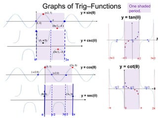
75. Graphs of Trig–Functions
Sine is periodic so we may reciprocate one period of
the sine wave to get the graph y = csc().
Reciprocating the y-coordinates π0 2π
( π/2, 1)
(3π/2, –1 )
y=sin()
y=csc()
The graph of csc() is periodic with period 2π.
Since cos() is the left-shift of the sin(), so the graph
of sec() is the left shift of the graph of csc().
Here are the graphs of all six trig-functions.

76. π/2 3π/20 2π
(1, π/2)
One shaded
period.
0 2π
Graphs of Trig–Functions
0
y = csc()
y = sec()
y = tan()
(0, 1) (2π, 1)
(2π, 1)
(3π/2, –1 )
(3π/2, –1 )