SlideShare a Scribd company logo
1 of 50
Download to read offline
Worksheet Analysis
Sketch a graph of the polynomial f(x) = (x–2)3Compute the results of the following operations involving polynomials: 4.(5k4+2k3+8)–(k2+4)
5.(x+2)(x2 + 4x +2) 6.Rewrite the polynomial expression T = (–0.01897V + 25.41881 V2 – 0.42456 V3 + 0.04365 V4)/V Student does not recognize
quadratic function Student does not infer from graph intersections in creating equation How can you recognize a graph from each of the function
families? Which function family does this graph belong to? What is the general equation for a graph from this function family? How can you use
points on the graph to create your equation? 2.f(x) = (x)(x–1)3(x–2)(x–3)2Student does not use roots to create equation. Student does not use
multiplicity of roots to create equation. ... Show more content on Helpwriting.net ...
What clues does the way the graph interacts with the x–axis (intersects it, forms a tangent, or has a turning point on the x–axis) give for creating the
equation? 3.Student fails to create a cubic graph Student does not sketch correct intersection at (2,0) What information can be drawn from the exponent
in the equation? What point would the term (x–2) of a polynomial populate on a graph? What does the exponent reveal about the nature of the graph's
intersection with the
... Get more on HelpWriting.net ...
The Low Form Credit Risk Model
Specification of the model.
In this dissertation the focus is on the reduced form credit risk model to calculate the prices of the default–free zero–coupon bonds. In order to use this
model the specification of the models' parameters should be done. More precisely, the hazard rate risk–neutral model, recovery rate and a default–free
term structure should be chosen.
Hazard process.
There are several most popular approaches for hazard process estimation.
First approach defines the hazard process as a stochastic process with help of Vasicek and CIR processes. Another approach that underlies the
cross–sectional estimation considers the hazard process to be either a stochastic or a constant. When the hazard rate is a stochastic process, there ...
Show more content on Helpwriting.net ...
First way is to estimate it is a parameter from a real market data and second way is to assume this rate as a constant. From the first point of view it
seems that the first method is more preferable than the second one, it is difficult and consuming in implementation.
The following graph shows a model obtained from the following security: a bond issued by Deutsche Bank that was taken from Bloomberg on the 23d
of July. The swap curve was used in the following graphs as a proxy for the default–free curve for a constant hazard rate model. The curves are built for
a constant recovery rates that vary from 10%–90% with a step of 10%. For each obtained value the hazard rate is estimated.
Graph 1. Graph one represents the fitted zero–coupon curve obtained from the Deutsche Bank bond from the bid quotes. The vertical axes is the
zero–coupon rate and the horizontal axes is time to maturity. The curve was calculated by Nelson–Siegel method in Matlab (see Appendix 1).
Graph 2. The second graph is function of 1 – recovery rate where recovery rate changes from 10% to 90%. The vertical axes values of the function
one minus recovery rate, meanwhile the horizontal axes shows the values of the recovery rate.
Graph 3. The third graph shows the hazard rate function that, as it was mentioned earlier, is a polynomial function of time to maturity and parameters
О»_i for i=1,...,n. The horizontal axes shows the recovery rate values, meanwhile the
... Get more on HelpWriting.net ...
Tide Modelling
IB Mathematics Standard Level Portfolio Assignment Task I
Tide Modeling
Kelvin Kwok
In this modeling assignment, I will develop a model function for the relationship between time of day and the height of the tide. I will first show the
data in a table form copied from the assignment sheet. Then I will use the data to construct a scatter graph of time against height, then I will develop a
function that models the behavior noted in the graph analytically, and describe any variables, parameters or constraints for the model. In the end I will
modify the same model using the regression feature of graphing software to develop a best–fit function for the data. This modeling task will allow me
to find out what is the best time that a good ... Show more content on Helpwriting.net ...
And for the value of C which is the horizontal translation, by trial and error method, I have found that by + ПЂ12 to the function which translate the
function to the left along the x–axis.
And D is the principal axis, as the min. value and max. value has already changed, so the new value for D would be 12.15+0.82=6.475
Hence we will get a modified function y=5.675sinx2+ПЂ12+6.475
Diagram3 Graph of the modified function y=5.675sinx2+ПЂ12+6.475 in method4
From diagram 3, we can see that the modified function has passed through 11 data points in total, which is 3 times more than the old function. So it is
obvious a better fit to the data points.
Method 5: Decide what time a good sailor should launch their boat based on the model in method 4
An outgoing tide is a receding tide , i.e. a tide that decreases from it's max height(crest) to its min. height(trough), from our observations on the graph
in method 4 , the max. height of the tide occurs at 2.6 hours after midnight and 15.2 hours after midnight which is 2:36am and 3:12pm respectively.
However, it's more sensible to launch a boat in day light rather than in the dark, therefore the best for a good sailor to launch a boat would be 3:12pm.
But since the function modeled in part 4 is not a perfit fit, therefore the perdiction of the best time to launch a boat is a theoretical guess.
... Get more on HelpWriting.net ...
Decibel Portfolio Essay
The intensity I of a sound wave is measured in watts per metre squared ( ). The lowest intensity that the average human ear can detect, i.e. the
threshold of hearing, is denoted by , where . The loudness of sound, i.e. its intensity level , is measured in decibels (dB), where . From this function a
specific relationship between and can be drawn that holds true for any increase in intensity. By knowing the value of beta ( ), the value of can be
found via manipulation of the logarithmic function, and by knowing the value of beta can by found by just taking the log of and multiplying it by ten.
The intensity level of ordinary conversation is 65 dB. In order to find the intensity of normal conversation on must set beta to 65 dB and to . ... Show
more content on Helpwriting.net ...
The values denoted by an * are values that were inserted during the investigation for this project. The process to find the values of Intensity with a
given Intensity Level was already mentioned, but the process in order to find Intensity Level by knowing the Intensity of a sound was not. In order to
find intensity level beta (b) from the equation one just takes the logarithm of and multiplies it by ten. The finding of the intensity level of a quiet radio
by knowing its intensity will be the example to test the method.
After carrying out this process and the other to find all the missing values, a relationship between the increase of the values can be discerned. By
carefully analyzing the table above, it can is concluded that while Intensity Level increase ten units, Intensity increase 10 times. By using a graphing
utility
... Get more on HelpWriting.net ...
What Do Graphs Look Like?
Lesson Four
Comparing Offers 2–3 Days (adapted from Irvine Math Project/ HCPSS Secondary Mathematics Office (v2); adapted from: Stephen Leinwand
Accessible mathematics: 10 instructional shifts that raise student achievement).
Content Standards: 8.F.A.2 Compare properties of two functions each represented in a different way (algebraically, graphically, numerically in tables,
or by verbal descriptions.)
Learning Objectives: Students will be able to explain and compare two equations and what they mean in the context of the problem. Students will be
able to decide if it is a better business decision to take Mr. Jones' job offer.
Materials Needed:
Initial scenario and Mr. Jones's scenario
Multiple representations graphic organizer
Colored pencils
Graph paper
Chart paper
Markers
Computer
Anticipatory Set: Have students complete a think–pair–share review of their understanding of the ... Show more content on Helpwriting.net ...
Graphing Function Applet Activity– Using the given scenario, pairs will complete the graphing investigation on the computer applet (http://cs.jsu.edu
/~leathrum/Mathlets/grapher.html). Consider having the following questions on a sheet for students to answer as a pair: What do the graphs look
like? Have them draw a sketch of the graphs. Have students consider the realistic values for x and y. Have students find the y–intercept for both
functions.
b.Graphing Calculator Activity – Pairs will use the graphing calculators to graph the functions. Pairs will enter the equations into the calculator. What
do the graphs look like? Have them draw a sketch of the graphs. Have students write a conjecture based on what they have seen with the graphs of the
two functions. Teachers should help students adjust the window so the x–min and y–min are zero, since you cannot have negative values. Have
students consider the reasoning behind values being less than zero. Since x–max is the number of hours worked, have students think about realistic
values.
Graphing
... Get more on HelpWriting.net ...
Core Curriculum Writing Assignment: A Quadratic Function
Devon Sparrow Instructor: Ralph Best MATH–1332 17 November 2015 Core Curriculum Writing Assignment: Quadratic function This paper will
discuss all possible graphs of a quadratic function, how to know when you have found them all, and the roles of the intercepts and coefficients and
how they affect the graphing of a quadratic function (Core Curriculum math sample writing assignment). The form of a quadratic function is
f(x)=ax^2+bx+c (Quadratic Functions). The U shape formed by the graph is called a parabola (Quadratic Functions). A quadratic function can be
graphed to open either up or down (Stewart, Ingrid). The coefficient is "a" (Stewart, Ingrid). If the coefficient is negative the graph will open down
(Stewart, Ingrid). If it is positive the graph will open up (Stewart, Ingrid). If the graph opens up "a" is greater than 0 and if the graph opens down "a"
is less than 0. In a quadratic function there are no more than 3 intercepts. 2 x intercepts and 1 y intercept. There are not always 2 x intercepts but there
is always a y intercept (Stewart, Ingrid). Knowing where the intercepts are helps to determine exact... Show more content on Helpwriting.net ...
Also mentioned was how to graph a quadratic function and information on the vertex and axis of symmetry. Works Cited "Quadratic Functions."
Quadratic Functions. N.p., n.d. Web. 17 Nov. 2015. http://dl.uncw.edu/digilib/mathematics/algebra/mat111hb/pandr/quadratic/quadratic.html#Content
"Core Curriculum Math Sample Writing Assignment". Handout. (Professor Ralph Best). Alvin Community College. Print. Stewart, Ingrid. "Quadratic
Functions." Quadratic Functions. N.p., n.d. Web. 17 Nov. 2015. http://sites.csn.edu/istewart/mathweb/math126/quad_func/quad.htm "Graphing
Quadratic Functions: Introduction." Graphing Quadratic Functions: Introduction. PurpleMath, n.d. Web. 17 Nov. 2015.
... Get more on HelpWriting.net ...
Math Sl Fish Production
FISH PRODUCTION – MODELING The aim of this investigation is to consider commercial fishing in a particular country in two different
environments, that is from the sea and a fish farm (aquaculture). The following data provided below was taken form the UN Statistics Division
Common Database. The tables gives the total mass of fish caught in the sea, in thousands of tones (1 tone = 1000 kilograms). Year| 1980| 1981| 1982|
1983| 1984| 1985| 1986| 1987| 1988| Total Mass| 426.8| 470.2| 503.4| 557.3| 564.7| 575.4| 579.8| 624.7| 669.9| Year| 1989| 1990| 1991| 1992| 1993| 1994|
1995| 1996| 1997| Total Mass| 450.5| 379.0| 356.9| 447.5| 548.8| 589.8| 634.0| 527.8| 459.1| Year|
... Show more content on Helpwriting.net ...
The principle axis is midway between the maximum and minimum, so d≈634.0+356.92≈495.45. So, the model is
M≈138.75sin2П
Ђ9x–c+495.45 for some constant c. We can notice that the point A on the original graph, graph1, lies on the principles axis and
so it is a point at which we are starting a new period. Since A is at (1989,450.5), c = 1989. The model is therefore
M≈138.75sin2П
Ђ9x–1989+495.45 and we can superimpose it on the original data as follows. Graph5. Sin model The graph shows what happens
when we fit the original graph , Graph4. with its model graph. The slopes of the two graphs are presented to be nearly equal at certain points. The
model presents decreasing and increasing values. Points shown from year 1989 – 1991, 1995 – 1997, 1999 – 2000, 2002 – 2003, 2004 –2005 are
decreasing, as for the rest of the years are increasing. The following table below presents the total mass of fish that were raised form the fish farm, in
thousands of tones. Year| 1980| 1981| 1982| 1983| 1984| 1985| 1986| 1987| 1988| Total Mass| 1.4| 1.5| 1.7| 2.0| 2.2| 2.7| 3.1| 3.3| 4.1| Year| 1989| 1990|
1991| 1992| 1993| 1994| 1995| 1996| 1997| Total Mass| 4.4| 5.8| 7.8| 9.1| 12.4| 16.0| 21.6| 33.2| 45.5| Year| 1998| 1999| 2000| 2001
... Get more on HelpWriting.net ...
Derivative and Graph
CALCULATOR SECTION
1. For find at the point (3, 4) on the curve.
A. B. C. D. E.
2. Suppose silver is being extracted from a mine at a rate given by , A(t) is measured in tons of silver and t in years from the opening of the mine.
Which is an expression for the amount of silver extracted from the mine in the first 5 years of its opening?
A. B. C. D. E.
3. Joe Student 's calculus test grades (G) are changing at the rate of 2 points per month. Which is the expression that says this?
A. B. C. D. E.
4. If f is a continuous and differentiable function, then approximate the ... Show more content on Helpwriting.net ...
A. Points A and BB. Points A and D C. Points B and DD. Points B and C E. Points A and C
18.
The graph of is shown above, on the interval [ –5, 5] . Which is true?
A. The graph is continuous and differentiable. B. The graph is continuous but not differentiable. C. The graph is not continuous but is differentiable. D.
The graph is not continuous nordifferentiable.
19. Graph in the plane above, over the window [–1, 8] X [–25, 25].
20. Give the x–interval(s) where the graph of g is increasing. GIVE A REASON for your answer.
21. Give the x–interval(s) where the graph of g is concave up. GIVE A REASON for your answer.
22. Give the x–coordinates of any critical points for the graph of g. For each tell if it is a relative maximum, a relative minimum or neither. EXPLAIN.
23. Give the x–coordinate of any points of inflection of the graph of g.
24. If is the velocity function for a particle moving along the x–axis, for time seconds, tell ...
A. when the particle changes direction. for .
B. for what intervals of time () the particle is moving to the left.
C. for what intervals of time
... Get more on HelpWriting.net ...
Math 30 IB Standard Level Body Mass Index Portfolio...
This portfolio is an investigation into how the median Body Mass Index of a girl will change as she ages. Body Mass Index (BMI) is a comparison
between a person's height (in meters) and weight (in kilograms) in order to determine whether one is overweight or underweight based on their
height. The goal of this portfolio is to prove of disprove how BMI as a function of Age (years) for girls living in the USA in 2000 can be modeled
using one or more mathematical equations. This data can be used for parents wanting to predict the change in BMI for their daughters or to compare
their daughter's BMI with the median BMI in the USA.
The equation used to measure BMI is:
The chart below shows the median BMI for girls of different ages in the ... Show more content on Helpwriting.net ...
That can be fixed by adjusting the horizontal phase shift value of _c_ to 12.4 to compensate.
There is also a noticeable discrepancy between the function graph and the scatter plot in the domain {} and {}. A slight stretch about the y axis would
fit the curve closer to the data points in those areas, therefore the _b_ value should be changed from ПЂ/15 to ПЂ/14. The number ПЂ/14 was chosen
because reducing the denominator's value by 1 will increase the b value by a slight amount, and an increased b value will shorten period and compress
the graph about the y axis, resulting in the values within domain to be closer to that of the data points.
Making these changes, the revised formula for the sinusoidal function is as follows:
Using TI InterActive!в„ў to graph that function, overlaid with the original data, and restricting the graph of the function to the same domain and range
as the domain and range on the scatterplot, the graph is as follows:
The refined equation fits the data much more closely at the beginning, yet around the Age = 13 mark it starts to deviate again. Looking at this graph,
one can come to the conclusion that it will take more than one mathematical function to graph the entirety of the data.
If one were to relate the concept of human growth with the measurable
... Get more on HelpWriting.net ...
Non-Function Piece-Wise Function Paper
For my "Non–function Piece–wise Function" project, I decided to use a miniature Christmas tree as my object. Right after tracing the object onto my
graph paper, I calculated the equation of each line segment. In order to find the equations of each line segment, I first had to find the slope of the
lines. To find the slope, I picked two obvious points from a line segment and plugged it into the slope equation. Finally, I plugged in the slope that I
figured out into the "point–slope form" equation along with one point of my choice, and finally got the equation. There was a particular error which I
bumped into during my analysis. At first, I had a plan to use a star as my object. But there was a problem. When I traced the
... Get more on HelpWriting.net ...
Role Of Cosine In The Simpsons
In this project I was able to utilize my knowledge about functions in order to create an image that represent the cosine and sine graphs as well as other
trigonometric graphs. Moreover, this project was really amusing because I had the opportunity to draw an image that represent the given graphs. The
reason I choose to do this image was first based on the cartoonish character Bart of the famous animated comedy The Simpsons. After analyzing the
character, I change many of its features such as the mouth, nose, eyebrows, and other elements. Furthermore, I changed the eyebrows and nose and
convert them into cosine curves. Similarly, I changed the mouth, hair and the sleeves of the shirt of my character into sine curves. In order to find the
equation
... Get more on HelpWriting.net ...
Spring Break Project Case Study
Our first step in completing the Spring Break Project was choosing a car, and since the four of us will be traveling a long distance, we decided that a
luxury car would be the best option. Once we decided, we found the cost for renting a luxury car for each of the companies and created functions to
represent the total cost. Those functions are as follows: y = 0.18x + 308 for Hertz, y = 0.13x + 426 for Enterprise, y = 0.15x + 364 for Dollar, and y =
0.20x +326 for Avis. We created these formulas by using the cost per mile as the slope, or the number multiplied by x, and used the initial cost as the
y–intercept, which is the number added. When the formulas had been created, we went on to making our graphs and tables up to 3,000 miles. We used
the tables to analyze our data, and found that Hertz offers the best initial offer up to 2,000 miles. After 2,000 miles, Dollar becomes the best option,
and at 3,250 we found that Enterprise becomes the best offer. We used our graph to double check this information, and found that after 3,250 miles,
Enterprise is the best option indefinitely. ... Show more content on Helpwriting.net ...
The three locations we chose were Myrtle Beach, New York City, and San Francisco. In order to find out how many miles a trip to each city would
be, we doubled the distance from Greensboro (where we would pick up the car) to the city to represent the round trip, and added 20 miles to that total
in case of detours or in–city travelling. This meant that a trip to Myrtle Beach would 412 miles, New York City would be 1,098, and San Francisco
would be 5,552 miles. To find the cost for each of these trips, we solved each function for the mileage of each city. Hertz had the bestprice for Myrtle
Beach and New York City, at $382.16 and $505.64, respectively. However, Enterprise was the best choice for San Francisco, only costing
... Get more on HelpWriting.net ...
Mathematics and Calculations
Running Head: MATHEMATIC AND CALCULATIONS
1.
a) ix=x–1+2
Transformation: The graph is shifted one unit to the right
b) jx=x+3
Transformation: The graph is shifted two units to the left
c) hx=x+3
Transformation: The graph is shifted three units along the x– axis
d) gx= – x
Transformation: the graph is transformed at an angle of 1800
2. Since no real numbers can be a square root of a negative number, the domain of f consist of all real numbers x such that;
4x+12 0
Therefore determining the domain of f is the same as solving the inequality
Let
hx= 4x+12 0 hx= 4x+12
4x=12
x 3
D= [3, )
Therefore the domain of f is all real numbers in the closed interval of 3 and infinity Set the denominator to zero (0) x+12=0x=–12 The domain
therefore is all real numbers greater than or less than –12
D= [ , –12) In this case there are no denominators therefore there is no division by zero
There is also no radical therefore there is no square root of a negative
Therefore the domain will be all real numbers The domain will be all real numbers except 0
This is because 1/0 is undefined
[15, ) x–15 0 x 15
3. Vertical asymptotes
Steps
The function for the vertical asymptote is first written down. In normal cases it should be a rational function and it should have a variable x in its
denominator. Always the vertical asymptote occurs when the denominator of the rational function is nearing zero
The second step is to find the value of x which makes the denominator
... Get more on HelpWriting.net ...
Consumer Behaviour of Purchasing Digital Camera
1.0 Introduction
In order to market the product into the market successfully, marketers need to have some marketing strategy to enter the desired market and make
profit. Market segmentation is the process of dividing a market into subsets of consumers with common needs or characteristics (Schiffman et al.,
2011). Understanding the market size and segmentation is valuable, but the keys to effective targeting is to know just how valuable specific consumer
groups are, and being able to quantify the impact of consumer trends ( Berry, 1999).
The purpose if this paper is to define the market segmentation for digital camera. Especially focus on Nikon digital camera which is the chosen product
in ... Show more content on Helpwriting.net ...
According to the consumer feedback survey conducted by Nikon in 2011, the consumers considered Nikon digital camera as user–friendly, affordable
price, well performance and good quality. The significant signal to explain this stage can be affordable price and good quality of the product.
2.1.2. Product benefits
After the product attributes it goes to the second stage which is product benefits. There are two consequences can discussed under the field of product
benefits, namely as functional consequences and psychosocial consequences.
The functional consequences is the tangible consequences of the product, it focus more on "what function is perform?'Also, it can be considered as an
external influence to the consumer. In this case the consequences may be user–friendly and excellence photographic performance.
The psychosocial consequence is a combination of psychological and social consequences. It emphasized more on 'How I feel?' and 'How people feel
about me?'which is more likely to be the internal influences to the consumers. Attraction and communication are significantly elements in this part. For
example, Nikon consumer may feel they catch people attention when they are using Nikon digital camera which is the psychological consequence.
Also the consumer may feel happy when they are using Nikon digital camera with others and create positiveexperience about the product, this may
considered as social consequence.
2.1.3 Personal values
The last
... Get more on HelpWriting.net ...
Analysis of Two Sets of Historical Data to Construct and...
ASSIGNMENT PART A EXECUTIVE SUMMARY The objective of this report is to analyze two sets of historical data and construct an
appropriate survival model to evaluate the behaviour of the two separate subjects. The process of modelling for the medflies included:
1.Preliminary data analysis to find and plot the empirical hazard and survival functions from the raw data based on a study on mortality rates of
medflies 2.Fitting and analyzing a Gompertz survival model, and by using least squares to find the parameters 3.Considering the Weibull as an
alternative model that would fit the empirical data more appropriately 4.The optimal models chosen in steps two and three was analyzed against
the empirical data on medflies in software R for analysis and the reasons as to why the models don't entirely fit with the empirical data. The second
set of data is based on a group of inmates analyzed after release from Maryland State prisons in the early 1970s based on several covariates. The
process of modelling for this set of data included: 1.Looking at the Kaplan–Meier estimate of the survival function and the empirical hazard function
without covariates 2.Considering the arrest times for African Americans against other races by ignoring effects of other covariates and analyzing the
difference. 3.Fitting a regression model to the arrest time information with all covariates; the error distribution for the model is also looked at, along
with which covariates were
... Get more on HelpWriting.net ...
The Effects of Varying Horizontal G-Forces
Introduction This is a look into the effects of varying horizontal G–Forces that are exposed to us and the amount or limit a human can tolerate of the
horizontal G–Forces. Charts and graphs that will represent the data will lend to a more authentic and concrete conclusion. To demonstrate growth and
unknown variables, an equation will be crafted. Such variables will be labeled and shown on the visual representations. To aide in the analysis of the
information, calculations will be done with a graphing calculator as well as open–source software available here: HYPERLINK "http://my.hrw.com
/math06_07/nsmedia/tools/Graph_Calculator/graphCalc.html"http://my.hrw.com/math06_07/nsmedia/tools/Graph_Calculator/graphCalc.html.– Any
visual demonstrations will be applied to the paper via jpgs. Any calculations performed will follow a set and defined procedure detailed below. Task 1
The first table of data illustrates the tolerance human beings have to horizontal G–force. The task is to define appropriate variables and parameters and
identify any contraints to the data. Time (Min) +Gx (g) 0.01 35 0.03 28 0.1 20 0.3 15 1 11 3 9 10 6 30 4.5 Variables X–Axis will be labeled as +Gx in
gees while the Y–Axis will be labeled as Time, specifically minutes. There is no constant variable here as both Time and +Gx fluctuate in relation to
each other. The analysis does demonstrate that as length of time increases the amount of +Gx gees tolerated decreases. Parameters: In
... Get more on HelpWriting.net ...
The Mathematics Of Blood Alcohol Concentration
The Mathematics of Blood Alcohol Concentration
As I approached my sixteenth birthday, I began to study for my G1 written test in order to receive my drivers' licence. While doing a practice test, I
came across a statistic that stated, "In the United States in 2013, it was estimated that 10 076 people were killed in crashes that involved one or more
drunk drivers and 290 000 people were injured in these accidents ". I had heard a variation of this statistic many times, however I didn't truly grasp the
magnitude of these numbers until I began to reflect on the effects of driving under the influence. As a potential new driver, I was concerned about the
use of alcohol while driving so I began to wonder how toxins, specifically alcohol, react within our bodies. I also wondered how, or even if, this
interaction could be represented through the use of mathematical analysis.
In my research I discovered for myself a field known as pharmacokinetics, which is a branch of pharmacology that deals with the interactions of drugs
in our bodies. In pharmacokinetics, the interaction of alcohol with the body can be visually represented using a concentration–time graph, where the
concentration can be graphed as a function with respect to time in hours. The concentration in this case refers to Blood Alcohol Concentration (BAC),
which is the amount of alcohol in 100 mL of blood with units, mg/100mL, or often expressed as a percent. BAC is a means by which doctors can
determine a person's
... Get more on HelpWriting.net ...
MTT Project 1 Graphs With Application
MTT Project 1 (Graphs with application) Name: Mohamed Alzbeidi ID: 1054072 Section: 1 Function: Quadratic Function Instructor: Jaya Kumar A.
Introduction: Quadratic is the function that is used for a squared degree. In this function its graph is called a parabola. The graph of all quadratic
function is called a parabola its shape is basically a U shape it might be transformed or reflected or inversed witch might change the shape in some
cases The simplest quadratic function is: y(x)=X^2 Furthermore, the general form to the quadratic function is y=гЂ–axгЂ—^2+bx+c=0 In any case
where a quadratic function cannot be solved the quadratic formula is used x=(–bВ±в€
љ(b^2–4ac))/2a The Quadratic Inverse: y(x)=в€
љx... Show more
content on Helpwriting.net ...
The equation of the reflected graph is y=гЂ–– (x)гЂ—^2 Example: y(x)=гЂ––(2x–3)гЂ—^2+1 C. Combination of all transformations with its inverse:
Basic Function: y=–1/2 (2x–4)^2+2 Inverse Function: y(x)=2В±в€
љ(2–x)/в€
љ2 Full Graph including basic function its inverse and y = x D. Real life
situation Quadratic Function A ball shot can be made using the equation y=–0.гЂ–0281xгЂ—^2+2x+10 , Where x is distance traveled (in feet) and y
is the height (also in feet). How long was the throw? First we apply the quadratic formula x=(–2В±в€
љ(2^2 )–4(–0.281Г—10))/(2(–0.0281)) x=75.9 ft
x=–4.7 y=10 E. Summary Although quadratic functions do not seem difficult but it is related to most fields in science and examples can be made by
any shape or act that might represent the form of a parabola. Including, there are more complex polynomials than the quadratic but it seems that this
function is the best introduction to functions and there graphs. Recourses https://www.desmos.com/
... Get more on HelpWriting.net ...
Basic Econ Essay
Chapter 2 MCQ's 1) According to the Law of Demand, the demand curve for a good will A) shift leftward when the price of the good increases. B)
shift rightward when the price of the good increases. C) slope downward. D) slope upward. Answer: C 2) An increase in the price of pork will lead
to A) a movement up along the demand curve. B) a movement down along the demand curve. C) a rightward shift of the demand curve. D) a
leftward shift of the demand curve. Answer: A 3) An increase in consumer incomes will lead to A) a rightward shift of the demand curve for plasma
TVs. B) a movement upward along the demand curve for plasma TVs. C) a rightward shift of the supply curve for plasma TVs. D) no change of the
demand curve for plasma TVs. Answer:... Show more content on Helpwriting.net ...
B) no government regulations exist. C) demand curves are perfectly horizontal. D) suppliers will supply any amount that buyers wish to buy.
Answer: A 19) Once an equilibrium is achieved, it can persist indefinitely because A) shocks that shift the demand curve or the supply curve
cannot occur. B) shocks to the demand curve are always exactly offset by shocks to the supply curve. C) the government never intervenes in markets at
equilibrium. D) in the absence of supply/demand shocks no one applies pressure to change the price. Answer: D 20) If price is initially above the
equilibrium level, A) the supply curve will shift rightward. B) the supply curve will shift leftward. C) excess supply exists. D) all firms can sell as
much as they want. Answer: C 21) An equilibrium in a market is described by A) a price only. B) a quantity only. C) the excess supply minus the
excess demand. D) a price and a quantity. Answer: D 3 22) The above figure shows a graph of the market for pizzas in a large town. At a price of $14,
there will be A) no pizzas supplied. B) equilibrium. C) excess supply. D) excess demand. Answer: C 23) The above figure shows a graph of the market
for pizzas in a large town. At a price of $5, there will be A) excess demand. B) excess supply. C) equilibrium. D) zero demand. Answer: A 24) The
above figure shows a graph of the market for pizzas in a large town. What are the equilibrium price and quantity? A) p = 8, Q = 60
... Get more on HelpWriting.net ...
Simulation of Dynamic Responses of First Order and Second...
Objectives:
As part of the experiment requirements, we were required to simulate the dynamic response of a first order and a second order linear system with the
help of LabVIEW. One of our first objectives of this experiment was to observe the response of the first order system to the input step signal and then
relate it to the time constant of that specific first order system. The second objective of this experiment included observing the second order system to
the input step signal and then relating it to the damping ratio of the specific second order system. The third and most important objective of this
experiment was to use different functions of LabVIEW including loop execution control, LabVIEW formula node, LabVIEW graph, LabVIEW ... Show
more content on Helpwriting.net ...
A shift register was then used to store the y value for the next iteration (y(n–1)) in case of the first order system while a 2 stacked shift register, in case
of a second order system, was used to store the y values from previous iterations (y(n–1) and y(n–2)). A formula node was used in order to input the
formula required to program the algorithm for each of the first and second order systems respectively. After providing the required number inputs and
outputs (as per the requirement of each of the formula respectively), a waveform function was used to create the waveform data from the output data
and determine the time interval of the input waveform. After using an array to contain all the input and output waveforms, a graph indicator was
finally added to the VI to display the final graphical representation of the output data.
After saving, each of the VI were run separately set at different time constants (for the first order system) and different damping ratios and 100 Hz
undamped natural frequency (for the second order ratio).
Results:
After creating the VI for first order differential systems in LabVIEW, we ran the VI using five different time constant values (0.01, 0.03, 0.05, 0.07,
0.1) and received the following graphs:
Figure : LabVIEW generated graph of amplitude against time for
... Get more on HelpWriting.net ...
Three Basic Trig Functions Of Trigonometry
SIX BASIC TRIG FUNCTIONS
Trigonometry, stemming from the greek words trigonon and metron , is the branch of mathematics in which sides and angles within in a triangle are
examined in relation to one another. A right triangle has six total functions used in correlation to its angles, represented by the greek letter theta (Оё).
The primary operations are sine (sin), cosine (cos) and tangent (tan) which serve also as the reciprocal of cosecant (csc), secant (sec), and cotangent
(cot) in that order. All six have abbreviations shown in parenthesis. Sine is the trigonometric function that is equal to the ratio of the side opposite a
given angle (Оё) to the hypotenuse. Cosine is the ratio of the side adjacent to Оё to the hypotenuse. Tangent is the ratio of the opposite side from the
given angle to the adjacent side. These functions are used in order to calculate unknown angles or distances from some known and/or measured aspects
in a geometric figure.
BRIEF HISTORYTrigonometry began as a method born from necessity to model the motions of galactic objects in mathematical astronomy. In order to
predict their movements with geometric accuracy Hipparchus began the development of mathematical tools which would allow astronomers to convert
arc lengths to distance measurements. Many contribute Hipparchus as the father of trigonometry. He was the first to construct a table of values of a
trigonometric function and created the notion that all triangles as being inscribed into a circle
... Get more on HelpWriting.net ...
Qrb501
WEEK ONE PROBLEMS
QRB501
McConnell & Brue Text
Chapter 7: Study Question 12
The following table shows nominal GDP and an appropriate price index for a group of selected years. Compute real GDP. Indicate in each calculation
whether you are inflating or deflating the nominal GDP data.
[pic]
Chapter 8: Study Question 2
Suppose an economy's real GDP is $30,000 in year 1 and $31,200 in year 2. What is the growth rate of its real GDP?
[(31,200 – 30,000) / 30,000] * 100 = 4.00%
Assume that population is 100 in year 1 and 102 in year 2. What is the growth rate of GDP per capita?
(30,000 / 100) = 300.00
(31,200 / 102) = 305.88
[(305.88 – 300.00) / 300.00)] * 100 = 1.96%
Chapter 8: Study ... Show more content on Helpwriting.net ...
The AverageTotal Cost graph is the sum of average fixed cost plus average variable cost. The shape of the graph is a hybrid of the average fixed cost
and average variable cost graphs. At any point on the X–axis, the plot for average total cost will equal the sum of average fixed cost plus average
variable cost.
The Marginal Cost graph is a function of change in total cost divided by change in quantity produced. Marginal cost is the added cost of producing one
additional unit of production, or the savings in not producing one additional unit. The graph decreases until the fourth unit of production, and then
increases rapidly, as marginal cost is tied to total cost and is thus subject to the law of diminishing returns.
...Continued on next page
The Marginal Cost graph intersects the Average Total Cost graph and the Average Variable Cost graphs at their minimum points. As long as the cost of
producing one additional unit remains less than average total cost, the average total cost continues to fall. When marginal cost finally exceeds average
total cost, average total cost begins to rise in response. The same effect applies to the relationship between marginal cost and average variable cost.
c) Explain how the location of each curve graphed in question 7b would be altered if (1) total fixed cost had been $100 rather than $60 and (2) total
variable cost had been $10
... Get more on HelpWriting.net ...
Using Microsoft Excel And Microsoft Word
A quartic equation is a fourth–order polynomial equation of the form. Shortly after the discovery of a method to solve the cubic equation, Lodovico
Ferrari (1522–1565), a student of Cardano, found a way to solve the quartic equation. His solution is a testimony to both the power and the limitations
of elementary algebra. The objective of this project is to analyze a polynomial of degree four via various attributes using Microsoft Excel and Microsoft
Word. I was assigned a nuumber in class that resembles a fucntion provided on the list.
An end behavior on a graph basically talks about the tailends of the graph. You determine the end behavior by looking at which way the tailends are
pointing. The end behavior is the behavior of the graph ... Show more content on Helpwriting.net ...
Looking at my graph i can come to a conclusion that the left side of my graph is going upward so F(x) is approching positive infinity. The left side
isnt pointing upward or downward so i had to look at my equation to determine what f(x) is. Since the leading coefficient is negative the right side of
the graph is going down , so f(x) approches negative infinity.
Local extrema is basically all local maximums and minimums on a functions graph. Local extrema occurs at criticla points on the graph where the
derivative is zero or undefined. To find the exact number of a local extrema using your polynomial , first find the first derivative of f using the
power rule. Then you will set the derivative to zero and solve for x. The values you get are the critical points which is also your local extrema. To
find the local extrema in your calculator all you have to do is enter the equation into Y=. Then hit GRAPH and look for the max value first. To find
the max value just go to calculate and choose maximum. Then move your cursor to the left when they ask you for left bound and hit enter and it will
tell you that you locked the position and just repeat the bounds for the right side too. When it asks for guess just hit enter and the coordinates of he
max value will appear. I had atleast 4 local extrema.
A zero of a function is an input value that produces an output of zero and can also be referred to as, a root. An examples of this would be f(x)=
... Get more on HelpWriting.net ...
Finding A Bore Tide
Introduction:
Daylight hours are dependent on sunrise and sunset times for each day which are dependent on seasonal change. The number of daylight hours can be
represented by a periodic function. This periodic function can help Alaskan Council predict daylight hours for tourist travelling to watch their Bore Tide
. A Bore Tide is a tidal phenomenon in which the leading edge of the incoming tide forms a wave (or waves) of water that travels up a river or
narrow bay against the direction of the river or bay's current. Anchorage, Alaska is known for its famous Bore Tides. These bore tides occur at least
once a day during high and low tide. Yet, health warnings are applied to viewing bore tides during low tide. Tourists have died by getting... Show more
content on Helpwriting.net ...
(Refer to Appendix 5 for the graph of the function:L=417 sinвЃЎ[2ПЂ/365 (t–81)]+744). As a regression analysis the function itself was used to find
daylight hours. The hours were then compared to the original data points. This comparison resulted in a percentage error being recorded. (Refer to
Appendix 5 for the results of the function and percentage errors). The highest percentage error recorded was 7.35% on February 1st 2011. This error
could be because February has 29 days in a leap year but 2011 data was used. The error could also occur because only 24 data points were used, if more
data points were used a more precise graph would have been generated leaving less space for error.
Question 1e:
Simple deriving and calculus was used to verify that the equation L=417 sinвЃЎ[2ПЂ/365 (t–81)]+744 for when the longest and shortest day of the
year occur. The derivative of the function was started by using the chain rule(dy/dx=dy/du*du/dx). The derivative was found to be: dy/dx=2ПЂ/365
417 cosвЃЎ(2ПЂ/365 t–162ПЂ/365). dy/dx was made to equal 0 therefore the equation will end up looking like: 0=cosвЃЎ(2ПЂ/365 t–162ПЂ/365).
When dealing with a cos curve on a unit circle cos can only be 0 at 90 degrees (ПЂ/2) and 270 degrees (3ПЂ/2) therefore meaning that to find the
longest and shortest days (2ПЂ/365 t–162ПЂ/365) is made
... Get more on HelpWriting.net ...
Summary: Unit 2 Of College Algebra
After applying more of my critical thinking in solving some exercises while reading has been of a great effect to my learning process in unit 2 of
College Algebra. According to Stitz, C. & Zeager, J. (2011), During the second week of term 4, I could read and cover many topics but the text I
found difficult to read are firstly, Graphs of Polynomials that states where a0, a1, . . . , an are real numbers and n _ 1 is a natural number. According
to 3.2 definition where we can now think of linear functions as degree 1 (or first degree') polynomial functions and quadratic functions as degree 2 (or
second degree') polynomial functions. The end behavior of a function is a way to describe what is happening to the function values (the y–values) as
the x–values approach the `ends' of the x–axis.9 That is, what happens to y as x becomes small without bound and, on the flip side, as x becomes large
without bound. While reading to understand this concept, I took up and practice this convention as stated in the text at this point and considered when
plotting it graphically, it looks a bit complex to my understanding. All... Show more content on Helpwriting.net ...
The zeros of p are the solutions to x2 +1 = 0, or x2 = –1. The imaginary unit "i" satisfies the two following properties. Establishing that "i" does act as a
square root2 of –1, and property 2 establishes what we mean by the `principal square root' of a negative real number. After reading the textbook for
hours, I had no choice than to repeat the reading the passages twice because at the initial stage, I barely could understand every mathematical functions,
calculations, and graph of polynomial. I was able to read the text book twice in other to understand most part of the Graphs of polynomial, The Factor
Theorem and The Remainder Theorem, and the Complex Zeros and the Fundamental Theorem of
... Get more on HelpWriting.net ...
Distribution Of Minimum Spanning Trees
Distributed Verification of Minimum Spanning Trees
Authors: Amos Korman, Shay Kutten
Problem Statement: A graph and a tree is given as input in a distributed manner and the algorithm is should be able to verifiy if the tree is a Minimum
Spanning Tree (MST).
Detailed Explanation of the Problem Statement
Definitions
Spanning tree: A spanning tree of an undirected graph is a subgraph which is a tree and includes all the vertices of G.
Minimum Spanning Tree (MST) : A spanning tree of a graph whose weight (sum of weight of its edges) is less than or equal to the weight of all other
spanning trees of the graph.
Verification of a Spanning Tree: A graph and a tree is given as input and the algorithm should check if the tree is an MST for the graph.
In distributed verification of Minimum Spanning Trees, the input is provided in a distributed manner which means that each node of the graph knows
which of its edges belong to the tree. A node does not have any knowledge of the edges which do not emanate from it. The verification algorithm should
label the vertices of the graph so that every node, given its own label and the labels of its neighbours only is able to detect if these edges are MST
edges or not and whether the input tree is an MST.
Motivation
The motivation for working on verification algorithms is that verification is easier than computation. In a distributed setting verification is even more
important because the tree is given in a distributed manner and computing such a
... Get more on HelpWriting.net ...
Comparison Of Mean Square Error ( FFBP )
comparison of mean square error using feed forward back propagation (FFBP) and radial basis function(RBF) neural network algorithms are given in
table 5.2 for analysis of band pass FIR filter with hanning window.
Table 5.2 Comparison of mean square error using FFBP and RBF neural network algorithms used for cut off frequency calculation of band pass FIR
digital filter with hanning window
Test input
(Filter
Coefficient)hanning
Window (actual cut off
Frequency)Output of Artificial Neural Network
(calculated cut off frequency)Mean Square Error
(MSE)
FFBPRBFFFBPRBF h(n) fc1fc2fc1fc2fc1fc2fc1fc2fc1fc2 h1(n) .155.355.15528.35528.155.355.0000000784.000000078400 h2(n)
.215.415.21459.41459.215.415 ... Show more content on Helpwriting.net ...
Table 5.5 Comparison of mean square error using FFBP and RBF neural network algorithms used for cut off frequency calculation of band pass FIR
digital filter with kaiser window
Test input
(Filter
coefficient)Kaiser
Window (actual cut off
Frequency)Output of artificial neural network
(calculated cut off frequency)Mean Square Error FFBPRBFFFBPRBF h(n) fc1fc2fc1fc2fc1fc2fc1fc2fc1fc2 h1(n)
.155.355.15567.35567.155.355.0000004489.000000448900 h2(n)
.215.415.21418.41418.21498.41498.0000006724.0000006724.0000000004.0000000004 h3(n)
.275.475.27404.47404.27499.47499.0000009216.0000009216.0000000001.0000000001 h4(n)
.335.535.33475.53475.335.535.0000000625.000000062500 h4(n) .395.595.39593.59593.395.595.0000008649.000000864900 h5(n)
.455.655.45541.65541.455.655.0000001681.000000168100 h6(n) .515.715.5145.7145.515.715.000000250000002500 h7(n)
.575.775.57232.77232.575.775.0000071824.000007182400 h8(n) .635.835.63531.83531.635.835.0000000961.000000096100 h9(n)
.695.895.69439.89439.695.895.0000003721.000000372100
Table
... Get more on HelpWriting.net ...
Bouncy Ball Lab Report
In the Bouncy Ball Lab, my team conducted two experiment that looked at how rebound height was affected by different independent factors. In the
first experiment, we chose six different starting heights and measured the rebound height in order to calculate how bouncy our given ball was, also
called the rebound ratio. We then graphed our data and found an equation to model the relationship between starting height and rebound height. In the
second experiment, we allowed our bouncy ball to continue bouncing after an initial height of 200cm. Again, we graphed the rebound height as the
dependant variable on the y–axis, but our independent variable was the number of times the ball had bounced. we also found an equation to model this
relationship.
... Get more on HelpWriting.net ...
A Mathematical Model: An Idealization of a Real Problem
A mathematical model is an idealisation of a real problem. Mathematical models also allow predictions to be made in studies. These models are usually
expressed in functions. Graphs are then plotted from these functions and will be analysed. The mathematical model that will be studied in this
investigation is mainly the cubic function.
Cubic functions are equations that are expressed in the form of f(x)=ax3+bx2+cx+d where a≠0 and a,b,c and d are constants. There are usually two
stationary points and an inflection point in cubic functions. This inflection point can either be a stationary inflection point or a non–stationary
inflection point.
Cubic equations were known to the ancient Babylonians, Chinese, Greeks, Egyptians and Indians. Physicians and mathematicians in the past such as
Hippocrates , Diophantus , Menaechmus , Archimedes and many more have studied the cubic function.
The aim of this investigation is to investigate the relationship between the stationary points of a cubic polynomial and the point of inflection of cubic
functions .This investigation will also discuss the contexts of applying cubic models to the real life situations.
Several items were used in completing this investigation. A TI–84 plus calculator from Texas Instruments was used. A printer was also used in printing
the papers in this investigation
In this task, a real life situation is that the electricity used in a house is charged into an electricity bill. The electricity consumption in Australia
... Get more on HelpWriting.net ...
How Does The Band Pass Digital Filter Design Using Kaiser...
5.6Band Pass FIR Digital Filter Design using kaiser Window The band pass FIR digital filter has been analysed with hanning window by using
FDA tool in the MATLAB. The cut off frequency has been estimated by using nn tool. 5.6.1Training using Feed Forward Back Propagation (FFBP)
artificial Neural Network Algorithm for kaiser Window Figure 5.11: trained network for kaiser window with FFBP Figure 5.12: performance plot
for kaiser window with FFBP In above figure 5.12, it shows the performance plot of a FFBP neural network. This plot is result of MLP training
algorithm. Here after 7 epochs the mean square error is almost 0. That means the network is trained. Figure 5.13: regression plot for kaiser window
with FFBP Here figure 5.13... Show more content on Helpwriting.net ...
Figure 5.16 shows an error graph between hamming window output obtained from the FDA tool of MATLAB and feed forward back propagation
algorithm output obtained from nn tool of MATLAB. Figure 5.16: Error graph between desired cut–off frequencies and obtained cut–off frequencies
for hamming window with FFBP Figure 5.17 shows an error graph between hamming window output obtained from the
... Get more on HelpWriting.net ...
The Neural Network Model
In the present chapter determining the radius for a given resonant frequency of centre feed circular microstrip antenna has been estimated using the
FFBP ANN
In the present chapter the radius for a given resonant frequency of a centre feed circular microstrip patch antenna has been analysed using two layer
neural network structures FFBP ANN model. The Levenberg– Marquardt training algorithm and the transfer function tansig have been used to
implement the neural network model. The simulated values for training and testing the neural network model are obtained by analysing the circular
microstrip patch antenna using CST Microwave Studio Software (CST–MWS). The results obtained using ANNs are compared with the simulation
findings and found ... Show more content on Helpwriting.net ...
Figure 3.1 shows the training performance graph that indicates the best validation performance and number of epochs required to achieve the
minimum mean square error level. The number of epochs required for training the aforesaid neural network to achieve mean square error (MSE) is
668. The training time is 3 seconds and the training algorithm used in the analysis model is Levenberg – Marquardt training algorithm.
Figure 3.2 shows the training state of the FFBP ANN model, the training state condition is shown by 3 different graphs in the first graph gradient value
is shown at different epochs, in the next graph Mu which indicates the error values at different epochs are shown and the third figure shows the
validation check points at different epochs. All the three graphs are showing the values at epoch 674.
The network is tested for 10 patterns and the table 3.1 shows the comparison of results of CST and FFBP–ANN with 5 neurons for radius with the
variation of the resonant frequency of the circular patch microstrip antenna computing MSE function with constant substrate height and dielectric
constant.
The network is realized using FFBP architecture. In the model, developed for the analysis of radius there are 10
... Get more on HelpWriting.net ...
Math Sl Fish Production
FISH PRODUCTION –
MODELING
The aim of this investigation is to consider commercial fishing in a particular country in two different environments, that is from the sea and a fish
farm (aquaculture).
The following data provided below was taken form the UN Statistics Division Common Database. The tables gives the total mass of fish caught in the
sea, in thousands of tones (1 tone = 1000 kilograms). Year| 1980| 1981| 1982| 1983| 1984| 1985| 1986| 1987| 1988| Total Mass| 426.8| 470.2| 503.4|
557.3| 564.7| 575.4| 579.8| 624.7| 669.9|
Year| 1989| 1990| 1991| 1992| 1993| 1994| 1995| 1996| 1997| Total Mass| 450.5| 379.0| 356.9| 447.5| 548.8| 589.8| 634.0| 527.8| 459.1|
Year| 1998| 1999| ... Show more content on Helpwriting.net ...
Graph7. Model
The graph shows what happens when we fit the original graph , Graph6. with its model graph. The slopes of the two graphs are presented to be nearly
equal to each other, whereas at a certain places it presents variation in values. However it can clearly be seen that the function is constantly increasing.
By considering the two presented models, it can be seen that in Graph5. the possible trend will keep increasing and decreasing its values as the years
go by. The shown Graph7. shows the trends of the amount of fish caught will possibly keep on rising in the future as the years go by, however little
decreases way assure on the
... Get more on HelpWriting.net ...
Isis Essential Standards Week 30 Essay
ESSENTIAL STANDARDS
ASSESSMENTS
By: Isis Gill–Reid
GRAPHING TRIGONOMETRIC
FUNCTIONS
Amplitude, Period, Phase Shift, Horizontal Shift of Sine and Cosine
DEFINITION
The trigonometric functions are functions of an angle. They relate the angles of a triangle to the lengths of its sides. Trigonometric functions are
important in the study of triangles and modeling periodic phenomena, among many other application. Amplitude is half the distance between the
minimum and maximum values of the range of a periodic function with a bounded range. A graph that repeats after a fixed interval, which is a period,
of the independent variable. Horizontal shift is obtained by determining the change being made to the x value. A phase shift represents the... Show more
content on Helpwriting.net ...
If a sequence of values follows a pattern of adding a fixed amount from one term to the next, it is referred to as an arithmetic sequence.
Examples
Arithmetic
Sequence
Common Difference, d d add 3 to each term to arrive at the next term, or...the difference a2
– a1 is 3.
1, 4, 7, 10,
13, 16, ...
=3
15, 10, 5, 0,
–5, –10, ...
d=
–5
add –5 to each term to arrive at the next term, or...the difference a2
– a1 is –5. add–1/2 to each term to arrive at the next term, or....the difference a2 – a1 is –1/2.
REAL LIFE SITUATION
Arithmetic sequences and series are used every day by engineers, accountants, and builders.
GEOMETRIC SEQUENCES AND
SERIES
Geometric Sequence, Geometric Series
DEFINITION
If a sequence of values follows a pattern of multiplying a fixed amount times each term to arrive at the following term it is referred to as a geometric
sequence. The sum of the terms of a sequence is called a series.
EXAMPLE
Geometric Sequence
Common Ratio, r r 5, 10, 20, 40, ...
=2
multiply each term
by 2 to arrive
at the next
term or...divide a2
–11, 22, –44, 88, ...
by a1 to find the common ratio, 2.
r = –2
or...divide
multiply each term by –2 to arrive at the next term
.or...divide a2 by a1 to find the common ratio, –2. multiply each term by 2/3 to arrive at the next term a2 by a1 to find the common
... Get more on HelpWriting.net ...
Exponential, Or Cubic) Do You Believe Will Best Fit The Data?
Student Name: ____Chesey Colston ______ Date: _____12/3/2014_____ Class: Algebra 2 Explore Linear Models: Years of School Average
Weekly Paycheck Some high school 11 450 High school graduate 13 585 Some college 15 810 Bachelor's degree 17 1000 Master's degree 19 1250
Doctoral degree 21 1600 1) Which type of function (linear, exponential, or cubic) do you believe will best fit the data? Support your choice. My
choice would be a Linear Function because it doesn't go through an intersection like an exponential function would, it also wouldn't be a cubic function
because it is not curved. It has all straight lines. 2) Find the rate of change between the data points of these intervals: (High school graduate) and (Some
college) High... Show more content on Helpwriting.net ...
Describe the pattern you see in them. 4) Use exponential regression (or find a constant ratio) to determine an equation for the data. 5) Graph the
equation you wrote in step four superimposed over the original data. Comment on how well or how poorly the equation fits the data. 6) If the
rounds of forwarding continued in the same pattern, predict the round that would be first to end up sending the link to more than 50,000 people.
Explain how you came up with this prediction. Explore Cubic Models: Record the volumes. Size of Corner Cut Volume of the Box (lwh) 1 100 2
3 4 5 Graph the table of data. Use your graph to answer the questions that follow. 1) Which type of function (linear, exponential, or cubic) do you
believe will best fit the data? Support your choice. 2) Find the rate of change between the data points of these intervals: (Corner Cut 1) and (Corner
Cut 2) (Corner Cut 2) and (Corner Cut 3) (Corner Cut 3) and (Corner Cut 4) 3) What do the rate of change values you just calculated represent? Why
are some positive and some negative? 4) Use cubic regression to determine an equation for the data (or lwh where (12 – x) represents the sides and (x)
represents the height of the box). 5) Graph the equation you wrote in step four superimposed over the original data. Comment on how well or how
... Get more on HelpWriting.net ...
Gravity Lab
Gravity Lab The goal of the experiment was to identify the gravitational acceleration from the recorded distance(cm) vs time(sec) data of a fallen
object. The first step was to graph the distance–time graph from the data collected. Upon graphing the data, the best fit line was identified in order to
find the formula of the function. As the data is representative of a graphical parabola, a parabolic function was utilized to be the best fit trendline. The
function Positon=404.289cm/s^2(t^s) + 44.450cm/s(t) +4.876cm was identified. In the equation, 404.289cm/s^2(t) represents the slope of the parabolic
curve pertaining to the distance(cm) over time(sec) as the 4.876cm displays the y–intercept in which the function crosses the axis leading to the
resulting curve. From identifying the distance–time graph equation, the next step is to find the velocity of the set data. ... Show more content on
Helpwriting.net ...
However, in order to find a linear slope of a parabolic curve, the mathematical equation of distance/time^2 ( pertaining to the data as cm/s^2) is used to
produce the linearization of the distance–time graph. A linear distance–time graph is the equivalent of a velocity–time graph by identifying the slope of
the distance–time graph. Another best fit line (a linear trendline) was plotted within the newly charted velocity–time graph. The equation identified
through the trendline was Velocity=808.578cm/s^2 (t) +44.450 cm/s. The 44.450cm/s represents the point in which the linear data crosses the y–axis as
the y–intercept. Additionally, the 808.578cm/s^2 represents the slope of the velocity–time graph in which the acceleration can be
... Get more on HelpWriting.net ...
Blood Spatter Investigation Essay
Introduction: For my Mathematics Internal Assessment, I focused on how the diameter of a blood droplet was affected by the height in which
they were shot at. When I watch criminal shows, they always estimate a person's height by the way blood is spread out and I wondered if the
diameter of a droplet really did change with the height where they were shot at, and if it was an effective method of presuming the height where
the victim was hit at the time they were shot. This topic has always interested me as when I was younger, I wanted to be a forensic scientist and the
way they solved crimes always intrigued me. Specifically, the way they conducted tests at the crime scene such as blood spatter analysis. My aim is
to find how related the height of the bullet entry is with the diameter of a blood droplet,and by doing that I will have to conduct my own experiment
as there is no data for what I want to do. By the end I hope to... Show more content on Helpwriting.net ...
This is because, I did not choose a droplet at random, but rather I would choose one that fit best with how the experiment was going. This was also
because many of the droplets that occurred were too small to get a result from and it would result in the same diameter for them in each different
height I tried. Graph 1.1 – Graph to show the list of points I obtained from my results From these results I plotted a graph, which I expected would
give me a quadratic equation, however the shape I got was not exactly a curve. As such, I approached it a different way and used piecewise function,
which is a function defined by multiple sub–functions, each sub–function applying to a certain interval of the main function's domain. To calculate a
linear equation for x values 10 to 90 cm and a quadratic equation from x values 90 to 190 cm, which I would then add onto my
... Get more on HelpWriting.net ...
Ib Physics Ia
IB Physics Internal Assessment
Andy Tang
Research Question
In this internal assessment, I am given a cantilever to find the physical properties of it. I decide to investigate the relationship between the force I act
on one side of the cantilever and the maximum acceleration the tail can reach. This experiment will be also showing the elasticity of the cantilever.
Since I pull down one side of it and fixed the other side, when I cut the string, it will bounce up and down until all the internal energy is depleted.
Text books
Newton meter
Accelerometer
Equilibrium line
Materials 1) A piece of cantilever that is made by acrylic plastic (length:35.2cmВ±0.1; Width:4.0cmВ±0.1; thickness:0.2cmВ±0.1) 2) An accelerometer
(sensor; ... Show more content on Helpwriting.net ...
By considering the formula: Ep=kx2/2, when x (the displacement caused by deformation) cannot be changed any more, the potential energy will not be
changing. When there is no more energy added into the system, the acceleration will not change.
Raw Data Table Force (NВ±0.05)| Acceleration (ms^–2)(В±0.2)| | Trial 1| Trial 2| Trial 3| | max| min| max| min| max| min| 0.75 | 22.3 |–18.5 | 21.2 |
–15.3 | 25.7 | –26.1 | 1.00 | 40.6 | –36.3 | 36.9 | –42.5 | 35.6 | –35.2 | 1.25 | 48.7 | –43.4 | 46.6 | –37.2 | 40.7 | –39.3 | 1.50 | 52.7 | –55.6 | 52.0 | –41.7 |
49.1 | –45.9 | 1.75 | 55.3 | –52.7 | 57.3 | –53.0 | 50.2 | –48.3 | 2.00 | 64.7 | –57.5 | 66.8 | –55.0 | 65.6 | –56.1 | 2.25 | 69.8 | –59.7 | 67.3 | –61.2 | 65.3 |
–63.2 | 2.50 | 78.0 | –63.8 | 68.0 | –63.8 | 64.3 | –62.8 | 2.75 | 74.7 | –63.8 | 83.8 | –63.8 | 83.7 | –63.2 | 3.00 | 83.8 | –63.8 | 83.1 | –63.8 | 83.6 | –63.8 |
Force uncertainty: The least count of the Newton meter that I used is 0.25N. Although the interspace of each scale is wide enough for me to determine,
I was not able to control the tension force which I act on the Newton meter. This created the uncertainty of the force measurement. By noticing the
fluctuation of the indicator, I estimate the uncertainty of the force is about 0.05N.
Acceleration uncertainty: The data of the acceleration were
... Get more on HelpWriting.net ...
Essay On Linear Function
Usually, translation involves only moving the graph around. To get started, let'sconsider one of the simpler types of functions that you have graphed;
namely, quadratic functions and their associated parabolas. If you have been doing your graphing by hand, you have probably started noticing some
relationships betweenthe equations and the graphs. This is always true: To move afunction up, you add outside the function: f b are f moved up b units.
Moving the function down works the same way; f –b is f moved down b units. If you losetrack, think about the point on the graph where x = 0. The
first, flipping upside down, is found by takingthe negative of the original function; that is, the rule for this transformation is –f. To see how this ... Show
more content on Helpwriting.net ...
Typical homework problems on this topic ask you tograph the transformation of a function, given the original function, or else askyou to figure out the
transformation, given the comparative graphs. Sometimes you will be given a point, or a graph with clearly plotted points, andtold to translate the
point(s) according to some rule. In other words, they won'tbe giving you a function, per se, to move; instead, you will be given points to move, and
you will have to know how to flip them around the axis systemyourself. Given the following graph of f, graph the transformation –f – 3. I have no
formula forf, so I cannot cheat; I have to do the transformation myself, point by point. Theway the original graph is drawn, there are four clearly
plotted points that I canuse to keep track of things. If I move the plotted points successfully, then I canfill in the rest of the graph once I am done. Now
that I have moved all the points, Ican graphs the transformation. Then pick a point to move, and trace out the sequence of steps with yourpencil tip,
drawing in the translated point once you reach its final location. Once you have moved all of the points, you can draw in the transformation. The other
exercise type is when you are given two graphs, one being theoriginal function and the other being the transformed function, and you are askedto figures
out the formula for the transformation.
... Get more on HelpWriting.net ...
Sst4e Tif 07 Essay
Ch. 7 The Normal Probability Distribution 7.1 Properties of the Normal Distribution 1 Use the uniform probability distribution. MULTIPLE
CHOICE. Choose the one alternative that best completes the statement or answers the question. Provide an appropriate response. 1) High
temperatures in a certain city for the month of August follow a uniform distribution over the interval 64В°F to 92В°F. What is the probability that a
randomly selected August day has a high temperature that exceeded 69В°F? A) 0.8214 B) 0.1786 C) 0.4423 D) 0.0357 2) High temperatures in a
certain city for the month of August follow a uniform distribution over the interval 73В°F to 103В°F. Find the high temperature which 90% of the
August days exceed. A) 76В°F B) 100В°F C) 83В°F... Show more content on Helpwriting.net ...
You randomly sample 30 preschool children and find their weights to be as follows. 25 25 26 26.5 27 27 27.5 28 28 28.5 29 29 30 30 30.5 31 31
32 32.5 32.5 33 33 34 34.5 35 35 37 37 38 38 a) Draw a histogram to display the data. Is it reasonable to assume that the weights are normally
distributed? Why? b) Find the mean and standard deviation of your sample. c) Is there a high probability that the mean and standard deviation of your
sample are consistent with those found in previous studies? Explain your reasoning. Page 218 MULTIPLE CHOICE. Choose the one alternative that
best completes the statement or answers the question. 2) The graph of a normal curve is given. Use the graph to identify the value of Ој and Пѓ. 3 6
A) Ој = 12, Пѓ = 3 9 12 15 18 B) Ој = 3, Пѓ = 12 21 C) Ој = 12, Пѓ = 9 D) Ој = 9, Пѓ = 12 3) The normal density curve is symmetric about A) Its
mean B) The horizontal axis C) An inflection point D) A point located one standard deviation from the mean 4) The highest point on the graph of the
normal density curve is located at A) its mean B) an inflection point C) Ој + Пѓ D) Ој + 3Пѓ 5) Approximately ____% of the area under the normal
curve is between Ој – 3Пѓ and Ој + 3Пѓ. A) 99.7 B) 68 C) 95 D) 50 Determine whether the graph can represent a normal curve. If it cannot, explain
why. 6) A) The graph cannot represent a normal density function because it increases
... Get more on HelpWriting.net ...

More Related Content

Similar to Worksheet Analysis

Artifact3 allen
Artifact3 allenArtifact3 allen
Artifact3 allenallent07
 
Scientific calculator project in c language
Scientific calculator project in c languageScientific calculator project in c language
Scientific calculator project in c languageAMIT KUMAR
 
Chapter3 hundred page machine learning
Chapter3 hundred page machine learningChapter3 hundred page machine learning
Chapter3 hundred page machine learningmustafa sarac
 
Calculus_Early_Transcendentals,_second_Edition,_by_Sullivan_and.pdf
Calculus_Early_Transcendentals,_second_Edition,_by_Sullivan_and.pdfCalculus_Early_Transcendentals,_second_Edition,_by_Sullivan_and.pdf
Calculus_Early_Transcendentals,_second_Edition,_by_Sullivan_and.pdfCONSTRUCTION WORLD SOLUTION
 
APLICACIONES DE LA DERIVADA EN LA CARRERA DE (Mecánica, Electrónica, Telecomu...
APLICACIONES DE LA DERIVADA EN LA CARRERA DE (Mecánica, Electrónica, Telecomu...APLICACIONES DE LA DERIVADA EN LA CARRERA DE (Mecánica, Electrónica, Telecomu...
APLICACIONES DE LA DERIVADA EN LA CARRERA DE (Mecánica, Electrónica, Telecomu...WILIAMMAURICIOCAHUAT1
 
Master of Computer Application (MCA) – Semester 4 MC0079
Master of Computer Application (MCA) – Semester 4  MC0079Master of Computer Application (MCA) – Semester 4  MC0079
Master of Computer Application (MCA) – Semester 4 MC0079Aravind NC
 
Marco-Calculus-AB-Lesson-Plan (Important book for calculus).pdf
Marco-Calculus-AB-Lesson-Plan (Important book for calculus).pdfMarco-Calculus-AB-Lesson-Plan (Important book for calculus).pdf
Marco-Calculus-AB-Lesson-Plan (Important book for calculus).pdfUniversity of the Punjab
 
Mc0079 computer based optimization methods--phpapp02
Mc0079 computer based optimization methods--phpapp02Mc0079 computer based optimization methods--phpapp02
Mc0079 computer based optimization methods--phpapp02Rabby Bhatt
 
Calculus Application Problem #3 Name _________________________.docx
Calculus Application Problem #3 Name _________________________.docxCalculus Application Problem #3 Name _________________________.docx
Calculus Application Problem #3 Name _________________________.docxhumphrieskalyn
 
Matlab intro notes
Matlab intro notesMatlab intro notes
Matlab intro notespawanss
 
PRML Chapter 4
PRML Chapter 4PRML Chapter 4
PRML Chapter 4Sunwoo Kim
 
1 P a g e ME 350 Project 2 Posted February 26.docx
1  P a g e   ME 350 Project 2  Posted February 26.docx1  P a g e   ME 350 Project 2  Posted February 26.docx
1 P a g e ME 350 Project 2 Posted February 26.docxoswald1horne84988
 

Similar to Worksheet Analysis (14)

Artifact3 allen
Artifact3 allenArtifact3 allen
Artifact3 allen
 
Scientific calculator project in c language
Scientific calculator project in c languageScientific calculator project in c language
Scientific calculator project in c language
 
Chapter3 hundred page machine learning
Chapter3 hundred page machine learningChapter3 hundred page machine learning
Chapter3 hundred page machine learning
 
Calculus_Early_Transcendentals,_second_Edition,_by_Sullivan_and.pdf
Calculus_Early_Transcendentals,_second_Edition,_by_Sullivan_and.pdfCalculus_Early_Transcendentals,_second_Edition,_by_Sullivan_and.pdf
Calculus_Early_Transcendentals,_second_Edition,_by_Sullivan_and.pdf
 
2 simple regression
2   simple regression2   simple regression
2 simple regression
 
APLICACIONES DE LA DERIVADA EN LA CARRERA DE (Mecánica, Electrónica, Telecomu...
APLICACIONES DE LA DERIVADA EN LA CARRERA DE (Mecánica, Electrónica, Telecomu...APLICACIONES DE LA DERIVADA EN LA CARRERA DE (Mecánica, Electrónica, Telecomu...
APLICACIONES DE LA DERIVADA EN LA CARRERA DE (Mecánica, Electrónica, Telecomu...
 
working with python
working with pythonworking with python
working with python
 
Master of Computer Application (MCA) – Semester 4 MC0079
Master of Computer Application (MCA) – Semester 4  MC0079Master of Computer Application (MCA) – Semester 4  MC0079
Master of Computer Application (MCA) – Semester 4 MC0079
 
Marco-Calculus-AB-Lesson-Plan (Important book for calculus).pdf
Marco-Calculus-AB-Lesson-Plan (Important book for calculus).pdfMarco-Calculus-AB-Lesson-Plan (Important book for calculus).pdf
Marco-Calculus-AB-Lesson-Plan (Important book for calculus).pdf
 
Mc0079 computer based optimization methods--phpapp02
Mc0079 computer based optimization methods--phpapp02Mc0079 computer based optimization methods--phpapp02
Mc0079 computer based optimization methods--phpapp02
 
Calculus Application Problem #3 Name _________________________.docx
Calculus Application Problem #3 Name _________________________.docxCalculus Application Problem #3 Name _________________________.docx
Calculus Application Problem #3 Name _________________________.docx
 
Matlab intro notes
Matlab intro notesMatlab intro notes
Matlab intro notes
 
PRML Chapter 4
PRML Chapter 4PRML Chapter 4
PRML Chapter 4
 
1 P a g e ME 350 Project 2 Posted February 26.docx
1  P a g e   ME 350 Project 2  Posted February 26.docx1  P a g e   ME 350 Project 2  Posted February 26.docx
1 P a g e ME 350 Project 2 Posted February 26.docx
 

More from Lynn Weber

How To Write A Good Introduction Paragraph Owl
How To Write A Good Introduction Paragraph OwlHow To Write A Good Introduction Paragraph Owl
How To Write A Good Introduction Paragraph OwlLynn Weber
 
Using Quotes In An Essay - YouTube
Using Quotes In An Essay - YouTubeUsing Quotes In An Essay - YouTube
Using Quotes In An Essay - YouTubeLynn Weber
 
5 Paragraph Essay Outline Print Paragraph Essay
5 Paragraph Essay Outline Print Paragraph Essay5 Paragraph Essay Outline Print Paragraph Essay
5 Paragraph Essay Outline Print Paragraph EssayLynn Weber
 
How To Write An Essay Grades 6-8 - TCR2491 T
How To Write An Essay Grades 6-8 - TCR2491 THow To Write An Essay Grades 6-8 - TCR2491 T
How To Write An Essay Grades 6-8 - TCR2491 TLynn Weber
 
How To Write An Essay In Spanish No-Prep Lesson P
How To Write An Essay In Spanish No-Prep Lesson PHow To Write An Essay In Spanish No-Prep Lesson P
How To Write An Essay In Spanish No-Prep Lesson PLynn Weber
 
Debate Script Format
Debate Script FormatDebate Script Format
Debate Script FormatLynn Weber
 
Writer Of The Federalist Papers. One Of The Writer
Writer Of The Federalist Papers. One Of The WriterWriter Of The Federalist Papers. One Of The Writer
Writer Of The Federalist Papers. One Of The WriterLynn Weber
 
Rhetorical Essay Outline A Rhetorical Analysis E
Rhetorical Essay Outline A Rhetorical Analysis ERhetorical Essay Outline A Rhetorical Analysis E
Rhetorical Essay Outline A Rhetorical Analysis ELynn Weber
 
Critical Analysis Essay Sample. Critical Analysis E
Critical Analysis Essay Sample. Critical Analysis ECritical Analysis Essay Sample. Critical Analysis E
Critical Analysis Essay Sample. Critical Analysis ELynn Weber
 
Critical Essay Short Research Paper Sa
Critical Essay Short Research Paper SaCritical Essay Short Research Paper Sa
Critical Essay Short Research Paper SaLynn Weber
 
Personal College Admission Essay E
Personal College Admission Essay EPersonal College Admission Essay E
Personal College Admission Essay ELynn Weber
 
My Plans For The Future Essay Telegraph
My Plans For The Future Essay TelegraphMy Plans For The Future Essay Telegraph
My Plans For The Future Essay TelegraphLynn Weber
 
Fun English Learning Site For Students And Teachers - Th
Fun English Learning Site For Students And Teachers - ThFun English Learning Site For Students And Teachers - Th
Fun English Learning Site For Students And Teachers - ThLynn Weber
 
Printable Turkey Writing Paper (Thanksgiving Page
Printable Turkey Writing Paper (Thanksgiving PagePrintable Turkey Writing Paper (Thanksgiving Page
Printable Turkey Writing Paper (Thanksgiving PageLynn Weber
 
6 Best Images Of Pretty Border Lined Paper Printa
6 Best Images Of Pretty Border Lined Paper Printa6 Best Images Of Pretty Border Lined Paper Printa
6 Best Images Of Pretty Border Lined Paper PrintaLynn Weber
 
School Essay Conclusion Of Cause And Effect Essay
School Essay Conclusion Of Cause And Effect EssaySchool Essay Conclusion Of Cause And Effect Essay
School Essay Conclusion Of Cause And Effect EssayLynn Weber
 
Research Paper On Photography
Research Paper On PhotographyResearch Paper On Photography
Research Paper On PhotographyLynn Weber
 

More from Lynn Weber (17)

How To Write A Good Introduction Paragraph Owl
How To Write A Good Introduction Paragraph OwlHow To Write A Good Introduction Paragraph Owl
How To Write A Good Introduction Paragraph Owl
 
Using Quotes In An Essay - YouTube
Using Quotes In An Essay - YouTubeUsing Quotes In An Essay - YouTube
Using Quotes In An Essay - YouTube
 
5 Paragraph Essay Outline Print Paragraph Essay
5 Paragraph Essay Outline Print Paragraph Essay5 Paragraph Essay Outline Print Paragraph Essay
5 Paragraph Essay Outline Print Paragraph Essay
 
How To Write An Essay Grades 6-8 - TCR2491 T
How To Write An Essay Grades 6-8 - TCR2491 THow To Write An Essay Grades 6-8 - TCR2491 T
How To Write An Essay Grades 6-8 - TCR2491 T
 
How To Write An Essay In Spanish No-Prep Lesson P
How To Write An Essay In Spanish No-Prep Lesson PHow To Write An Essay In Spanish No-Prep Lesson P
How To Write An Essay In Spanish No-Prep Lesson P
 
Debate Script Format
Debate Script FormatDebate Script Format
Debate Script Format
 
Writer Of The Federalist Papers. One Of The Writer
Writer Of The Federalist Papers. One Of The WriterWriter Of The Federalist Papers. One Of The Writer
Writer Of The Federalist Papers. One Of The Writer
 
Rhetorical Essay Outline A Rhetorical Analysis E
Rhetorical Essay Outline A Rhetorical Analysis ERhetorical Essay Outline A Rhetorical Analysis E
Rhetorical Essay Outline A Rhetorical Analysis E
 
Critical Analysis Essay Sample. Critical Analysis E
Critical Analysis Essay Sample. Critical Analysis ECritical Analysis Essay Sample. Critical Analysis E
Critical Analysis Essay Sample. Critical Analysis E
 
Critical Essay Short Research Paper Sa
Critical Essay Short Research Paper SaCritical Essay Short Research Paper Sa
Critical Essay Short Research Paper Sa
 
Personal College Admission Essay E
Personal College Admission Essay EPersonal College Admission Essay E
Personal College Admission Essay E
 
My Plans For The Future Essay Telegraph
My Plans For The Future Essay TelegraphMy Plans For The Future Essay Telegraph
My Plans For The Future Essay Telegraph
 
Fun English Learning Site For Students And Teachers - Th
Fun English Learning Site For Students And Teachers - ThFun English Learning Site For Students And Teachers - Th
Fun English Learning Site For Students And Teachers - Th
 
Printable Turkey Writing Paper (Thanksgiving Page
Printable Turkey Writing Paper (Thanksgiving PagePrintable Turkey Writing Paper (Thanksgiving Page
Printable Turkey Writing Paper (Thanksgiving Page
 
6 Best Images Of Pretty Border Lined Paper Printa
6 Best Images Of Pretty Border Lined Paper Printa6 Best Images Of Pretty Border Lined Paper Printa
6 Best Images Of Pretty Border Lined Paper Printa
 
School Essay Conclusion Of Cause And Effect Essay
School Essay Conclusion Of Cause And Effect EssaySchool Essay Conclusion Of Cause And Effect Essay
School Essay Conclusion Of Cause And Effect Essay
 
Research Paper On Photography
Research Paper On PhotographyResearch Paper On Photography
Research Paper On Photography
 

Recently uploaded

ACC 2024 Chronicles. Cardiology. Exam.pdf
ACC 2024 Chronicles. Cardiology. Exam.pdfACC 2024 Chronicles. Cardiology. Exam.pdf
ACC 2024 Chronicles. Cardiology. Exam.pdfSpandanaRallapalli
 
Keynote by Prof. Wurzer at Nordex about IP-design
Keynote by Prof. Wurzer at Nordex about IP-designKeynote by Prof. Wurzer at Nordex about IP-design
Keynote by Prof. Wurzer at Nordex about IP-designMIPLM
 
Roles & Responsibilities in Pharmacovigilance
Roles & Responsibilities in PharmacovigilanceRoles & Responsibilities in Pharmacovigilance
Roles & Responsibilities in PharmacovigilanceSamikshaHamane
 
Earth Day Presentation wow hello nice great
Earth Day Presentation wow hello nice greatEarth Day Presentation wow hello nice great
Earth Day Presentation wow hello nice greatYousafMalik24
 
How to Configure Email Server in Odoo 17
How to Configure Email Server in Odoo 17How to Configure Email Server in Odoo 17
How to Configure Email Server in Odoo 17Celine George
 
Hierarchy of management that covers different levels of management
Hierarchy of management that covers different levels of managementHierarchy of management that covers different levels of management
Hierarchy of management that covers different levels of managementmkooblal
 
Crayon Activity Handout For the Crayon A
Crayon Activity Handout For the Crayon ACrayon Activity Handout For the Crayon A
Crayon Activity Handout For the Crayon AUnboundStockton
 
ECONOMIC CONTEXT - PAPER 1 Q3: NEWSPAPERS.pptx
ECONOMIC CONTEXT - PAPER 1 Q3: NEWSPAPERS.pptxECONOMIC CONTEXT - PAPER 1 Q3: NEWSPAPERS.pptx
ECONOMIC CONTEXT - PAPER 1 Q3: NEWSPAPERS.pptxiammrhaywood
 
Alper Gobel In Media Res Media Component
Alper Gobel In Media Res Media ComponentAlper Gobel In Media Res Media Component
Alper Gobel In Media Res Media ComponentInMediaRes1
 
HỌC TỐT TIẾNG ANH 11 THEO CHƯƠNG TRÌNH GLOBAL SUCCESS ĐÁP ÁN CHI TIẾT - CẢ NĂ...
HỌC TỐT TIẾNG ANH 11 THEO CHƯƠNG TRÌNH GLOBAL SUCCESS ĐÁP ÁN CHI TIẾT - CẢ NĂ...HỌC TỐT TIẾNG ANH 11 THEO CHƯƠNG TRÌNH GLOBAL SUCCESS ĐÁP ÁN CHI TIẾT - CẢ NĂ...
HỌC TỐT TIẾNG ANH 11 THEO CHƯƠNG TRÌNH GLOBAL SUCCESS ĐÁP ÁN CHI TIẾT - CẢ NĂ...Nguyen Thanh Tu Collection
 
ECONOMIC CONTEXT - LONG FORM TV DRAMA - PPT
ECONOMIC CONTEXT - LONG FORM TV DRAMA - PPTECONOMIC CONTEXT - LONG FORM TV DRAMA - PPT
ECONOMIC CONTEXT - LONG FORM TV DRAMA - PPTiammrhaywood
 
Solving Puzzles Benefits Everyone (English).pptx
Solving Puzzles Benefits Everyone (English).pptxSolving Puzzles Benefits Everyone (English).pptx
Solving Puzzles Benefits Everyone (English).pptxOH TEIK BIN
 
ENGLISH6-Q4-W3.pptxqurter our high choom
ENGLISH6-Q4-W3.pptxqurter our high choomENGLISH6-Q4-W3.pptxqurter our high choom
ENGLISH6-Q4-W3.pptxqurter our high choomnelietumpap1
 
call girls in Kamla Market (DELHI) 🔝 >༒9953330565🔝 genuine Escort Service 🔝✔️✔️
call girls in Kamla Market (DELHI) 🔝 >༒9953330565🔝 genuine Escort Service 🔝✔️✔️call girls in Kamla Market (DELHI) 🔝 >༒9953330565🔝 genuine Escort Service 🔝✔️✔️
call girls in Kamla Market (DELHI) 🔝 >༒9953330565🔝 genuine Escort Service 🔝✔️✔️9953056974 Low Rate Call Girls In Saket, Delhi NCR
 
Grade 9 Q4-MELC1-Active and Passive Voice.pptx
Grade 9 Q4-MELC1-Active and Passive Voice.pptxGrade 9 Q4-MELC1-Active and Passive Voice.pptx
Grade 9 Q4-MELC1-Active and Passive Voice.pptxChelloAnnAsuncion2
 
Proudly South Africa powerpoint Thorisha.pptx
Proudly South Africa powerpoint Thorisha.pptxProudly South Africa powerpoint Thorisha.pptx
Proudly South Africa powerpoint Thorisha.pptxthorishapillay1
 
Full Stack Web Development Course for Beginners
Full Stack Web Development Course  for BeginnersFull Stack Web Development Course  for Beginners
Full Stack Web Development Course for BeginnersSabitha Banu
 
Judging the Relevance and worth of ideas part 2.pptx
Judging the Relevance  and worth of ideas part 2.pptxJudging the Relevance  and worth of ideas part 2.pptx
Judging the Relevance and worth of ideas part 2.pptxSherlyMaeNeri
 

Recently uploaded (20)

ACC 2024 Chronicles. Cardiology. Exam.pdf
ACC 2024 Chronicles. Cardiology. Exam.pdfACC 2024 Chronicles. Cardiology. Exam.pdf
ACC 2024 Chronicles. Cardiology. Exam.pdf
 
Keynote by Prof. Wurzer at Nordex about IP-design
Keynote by Prof. Wurzer at Nordex about IP-designKeynote by Prof. Wurzer at Nordex about IP-design
Keynote by Prof. Wurzer at Nordex about IP-design
 
Roles & Responsibilities in Pharmacovigilance
Roles & Responsibilities in PharmacovigilanceRoles & Responsibilities in Pharmacovigilance
Roles & Responsibilities in Pharmacovigilance
 
Earth Day Presentation wow hello nice great
Earth Day Presentation wow hello nice greatEarth Day Presentation wow hello nice great
Earth Day Presentation wow hello nice great
 
How to Configure Email Server in Odoo 17
How to Configure Email Server in Odoo 17How to Configure Email Server in Odoo 17
How to Configure Email Server in Odoo 17
 
Hierarchy of management that covers different levels of management
Hierarchy of management that covers different levels of managementHierarchy of management that covers different levels of management
Hierarchy of management that covers different levels of management
 
OS-operating systems- ch04 (Threads) ...
OS-operating systems- ch04 (Threads) ...OS-operating systems- ch04 (Threads) ...
OS-operating systems- ch04 (Threads) ...
 
Crayon Activity Handout For the Crayon A
Crayon Activity Handout For the Crayon ACrayon Activity Handout For the Crayon A
Crayon Activity Handout For the Crayon A
 
ECONOMIC CONTEXT - PAPER 1 Q3: NEWSPAPERS.pptx
ECONOMIC CONTEXT - PAPER 1 Q3: NEWSPAPERS.pptxECONOMIC CONTEXT - PAPER 1 Q3: NEWSPAPERS.pptx
ECONOMIC CONTEXT - PAPER 1 Q3: NEWSPAPERS.pptx
 
Alper Gobel In Media Res Media Component
Alper Gobel In Media Res Media ComponentAlper Gobel In Media Res Media Component
Alper Gobel In Media Res Media Component
 
HỌC TỐT TIẾNG ANH 11 THEO CHƯƠNG TRÌNH GLOBAL SUCCESS ĐÁP ÁN CHI TIẾT - CẢ NĂ...
HỌC TỐT TIẾNG ANH 11 THEO CHƯƠNG TRÌNH GLOBAL SUCCESS ĐÁP ÁN CHI TIẾT - CẢ NĂ...HỌC TỐT TIẾNG ANH 11 THEO CHƯƠNG TRÌNH GLOBAL SUCCESS ĐÁP ÁN CHI TIẾT - CẢ NĂ...
HỌC TỐT TIẾNG ANH 11 THEO CHƯƠNG TRÌNH GLOBAL SUCCESS ĐÁP ÁN CHI TIẾT - CẢ NĂ...
 
ECONOMIC CONTEXT - LONG FORM TV DRAMA - PPT
ECONOMIC CONTEXT - LONG FORM TV DRAMA - PPTECONOMIC CONTEXT - LONG FORM TV DRAMA - PPT
ECONOMIC CONTEXT - LONG FORM TV DRAMA - PPT
 
Solving Puzzles Benefits Everyone (English).pptx
Solving Puzzles Benefits Everyone (English).pptxSolving Puzzles Benefits Everyone (English).pptx
Solving Puzzles Benefits Everyone (English).pptx
 
Rapple "Scholarly Communications and the Sustainable Development Goals"
Rapple "Scholarly Communications and the Sustainable Development Goals"Rapple "Scholarly Communications and the Sustainable Development Goals"
Rapple "Scholarly Communications and the Sustainable Development Goals"
 
ENGLISH6-Q4-W3.pptxqurter our high choom
ENGLISH6-Q4-W3.pptxqurter our high choomENGLISH6-Q4-W3.pptxqurter our high choom
ENGLISH6-Q4-W3.pptxqurter our high choom
 
call girls in Kamla Market (DELHI) 🔝 >༒9953330565🔝 genuine Escort Service 🔝✔️✔️
call girls in Kamla Market (DELHI) 🔝 >༒9953330565🔝 genuine Escort Service 🔝✔️✔️call girls in Kamla Market (DELHI) 🔝 >༒9953330565🔝 genuine Escort Service 🔝✔️✔️
call girls in Kamla Market (DELHI) 🔝 >༒9953330565🔝 genuine Escort Service 🔝✔️✔️
 
Grade 9 Q4-MELC1-Active and Passive Voice.pptx
Grade 9 Q4-MELC1-Active and Passive Voice.pptxGrade 9 Q4-MELC1-Active and Passive Voice.pptx
Grade 9 Q4-MELC1-Active and Passive Voice.pptx
 
Proudly South Africa powerpoint Thorisha.pptx
Proudly South Africa powerpoint Thorisha.pptxProudly South Africa powerpoint Thorisha.pptx
Proudly South Africa powerpoint Thorisha.pptx
 
Full Stack Web Development Course for Beginners
Full Stack Web Development Course  for BeginnersFull Stack Web Development Course  for Beginners
Full Stack Web Development Course for Beginners
 
Judging the Relevance and worth of ideas part 2.pptx
Judging the Relevance  and worth of ideas part 2.pptxJudging the Relevance  and worth of ideas part 2.pptx
Judging the Relevance and worth of ideas part 2.pptx
 

Worksheet Analysis

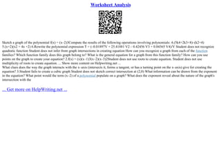
  • 1. Worksheet Analysis Sketch a graph of the polynomial f(x) = (x–2)3Compute the results of the following operations involving polynomials: 4.(5k4+2k3+8)–(k2+4) 5.(x+2)(x2 + 4x +2) 6.Rewrite the polynomial expression T = (–0.01897V + 25.41881 V2 – 0.42456 V3 + 0.04365 V4)/V Student does not recognize quadratic function Student does not infer from graph intersections in creating equation How can you recognize a graph from each of the function families? Which function family does this graph belong to? What is the general equation for a graph from this function family? How can you use points on the graph to create your equation? 2.f(x) = (x)(x–1)3(x–2)(x–3)2Student does not use roots to create equation. Student does not use multiplicity of roots to create equation. ... Show more content on Helpwriting.net ... What clues does the way the graph interacts with the x–axis (intersects it, forms a tangent, or has a turning point on the x–axis) give for creating the equation? 3.Student fails to create a cubic graph Student does not sketch correct intersection at (2,0) What information can be drawn from the exponent in the equation? What point would the term (x–2) of a polynomial populate on a graph? What does the exponent reveal about the nature of the graph's intersection with the ... Get more on HelpWriting.net ...
  • 2. The Low Form Credit Risk Model Specification of the model. In this dissertation the focus is on the reduced form credit risk model to calculate the prices of the default–free zero–coupon bonds. In order to use this model the specification of the models' parameters should be done. More precisely, the hazard rate risk–neutral model, recovery rate and a default–free term structure should be chosen. Hazard process. There are several most popular approaches for hazard process estimation. First approach defines the hazard process as a stochastic process with help of Vasicek and CIR processes. Another approach that underlies the cross–sectional estimation considers the hazard process to be either a stochastic or a constant. When the hazard rate is a stochastic process, there ... Show more content on Helpwriting.net ... First way is to estimate it is a parameter from a real market data and second way is to assume this rate as a constant. From the first point of view it seems that the first method is more preferable than the second one, it is difficult and consuming in implementation. The following graph shows a model obtained from the following security: a bond issued by Deutsche Bank that was taken from Bloomberg on the 23d of July. The swap curve was used in the following graphs as a proxy for the default–free curve for a constant hazard rate model. The curves are built for a constant recovery rates that vary from 10%–90% with a step of 10%. For each obtained value the hazard rate is estimated. Graph 1. Graph one represents the fitted zero–coupon curve obtained from the Deutsche Bank bond from the bid quotes. The vertical axes is the zero–coupon rate and the horizontal axes is time to maturity. The curve was calculated by Nelson–Siegel method in Matlab (see Appendix 1). Graph 2. The second graph is function of 1 – recovery rate where recovery rate changes from 10% to 90%. The vertical axes values of the function one minus recovery rate, meanwhile the horizontal axes shows the values of the recovery rate. Graph 3. The third graph shows the hazard rate function that, as it was mentioned earlier, is a polynomial function of time to maturity and parameters О»_i for i=1,...,n. The horizontal axes shows the recovery rate values, meanwhile the ... Get more on HelpWriting.net ...
  • 3. Tide Modelling IB Mathematics Standard Level Portfolio Assignment Task I Tide Modeling Kelvin Kwok In this modeling assignment, I will develop a model function for the relationship between time of day and the height of the tide. I will first show the data in a table form copied from the assignment sheet. Then I will use the data to construct a scatter graph of time against height, then I will develop a function that models the behavior noted in the graph analytically, and describe any variables, parameters or constraints for the model. In the end I will modify the same model using the regression feature of graphing software to develop a best–fit function for the data. This modeling task will allow me to find out what is the best time that a good ... Show more content on Helpwriting.net ... And for the value of C which is the horizontal translation, by trial and error method, I have found that by + ПЂ12 to the function which translate the function to the left along the x–axis. And D is the principal axis, as the min. value and max. value has already changed, so the new value for D would be 12.15+0.82=6.475 Hence we will get a modified function y=5.675sinx2+ПЂ12+6.475 Diagram3 Graph of the modified function y=5.675sinx2+ПЂ12+6.475 in method4 From diagram 3, we can see that the modified function has passed through 11 data points in total, which is 3 times more than the old function. So it is obvious a better fit to the data points. Method 5: Decide what time a good sailor should launch their boat based on the model in method 4 An outgoing tide is a receding tide , i.e. a tide that decreases from it's max height(crest) to its min. height(trough), from our observations on the graph in method 4 , the max. height of the tide occurs at 2.6 hours after midnight and 15.2 hours after midnight which is 2:36am and 3:12pm respectively. However, it's more sensible to launch a boat in day light rather than in the dark, therefore the best for a good sailor to launch a boat would be 3:12pm. But since the function modeled in part 4 is not a perfit fit, therefore the perdiction of the best time to launch a boat is a theoretical guess.
  • 4. ... Get more on HelpWriting.net ...
  • 5. Decibel Portfolio Essay The intensity I of a sound wave is measured in watts per metre squared ( ). The lowest intensity that the average human ear can detect, i.e. the threshold of hearing, is denoted by , where . The loudness of sound, i.e. its intensity level , is measured in decibels (dB), where . From this function a specific relationship between and can be drawn that holds true for any increase in intensity. By knowing the value of beta ( ), the value of can be found via manipulation of the logarithmic function, and by knowing the value of beta can by found by just taking the log of and multiplying it by ten. The intensity level of ordinary conversation is 65 dB. In order to find the intensity of normal conversation on must set beta to 65 dB and to . ... Show more content on Helpwriting.net ... The values denoted by an * are values that were inserted during the investigation for this project. The process to find the values of Intensity with a given Intensity Level was already mentioned, but the process in order to find Intensity Level by knowing the Intensity of a sound was not. In order to find intensity level beta (b) from the equation one just takes the logarithm of and multiplies it by ten. The finding of the intensity level of a quiet radio by knowing its intensity will be the example to test the method. After carrying out this process and the other to find all the missing values, a relationship between the increase of the values can be discerned. By carefully analyzing the table above, it can is concluded that while Intensity Level increase ten units, Intensity increase 10 times. By using a graphing utility ... Get more on HelpWriting.net ...
  • 6. What Do Graphs Look Like? Lesson Four Comparing Offers 2–3 Days (adapted from Irvine Math Project/ HCPSS Secondary Mathematics Office (v2); adapted from: Stephen Leinwand Accessible mathematics: 10 instructional shifts that raise student achievement). Content Standards: 8.F.A.2 Compare properties of two functions each represented in a different way (algebraically, graphically, numerically in tables, or by verbal descriptions.) Learning Objectives: Students will be able to explain and compare two equations and what they mean in the context of the problem. Students will be able to decide if it is a better business decision to take Mr. Jones' job offer. Materials Needed: Initial scenario and Mr. Jones's scenario Multiple representations graphic organizer Colored pencils Graph paper Chart paper Markers Computer Anticipatory Set: Have students complete a think–pair–share review of their understanding of the ... Show more content on Helpwriting.net ... Graphing Function Applet Activity– Using the given scenario, pairs will complete the graphing investigation on the computer applet (http://cs.jsu.edu /~leathrum/Mathlets/grapher.html). Consider having the following questions on a sheet for students to answer as a pair: What do the graphs look like? Have them draw a sketch of the graphs. Have students consider the realistic values for x and y. Have students find the y–intercept for both functions. b.Graphing Calculator Activity – Pairs will use the graphing calculators to graph the functions. Pairs will enter the equations into the calculator. What do the graphs look like? Have them draw a sketch of the graphs. Have students write a conjecture based on what they have seen with the graphs of the two functions. Teachers should help students adjust the window so the x–min and y–min are zero, since you cannot have negative values. Have students consider the reasoning behind values being less than zero. Since x–max is the number of hours worked, have students think about realistic values. Graphing
  • 7. ... Get more on HelpWriting.net ...
  • 8. Core Curriculum Writing Assignment: A Quadratic Function Devon Sparrow Instructor: Ralph Best MATH–1332 17 November 2015 Core Curriculum Writing Assignment: Quadratic function This paper will discuss all possible graphs of a quadratic function, how to know when you have found them all, and the roles of the intercepts and coefficients and how they affect the graphing of a quadratic function (Core Curriculum math sample writing assignment). The form of a quadratic function is f(x)=ax^2+bx+c (Quadratic Functions). The U shape formed by the graph is called a parabola (Quadratic Functions). A quadratic function can be graphed to open either up or down (Stewart, Ingrid). The coefficient is "a" (Stewart, Ingrid). If the coefficient is negative the graph will open down (Stewart, Ingrid). If it is positive the graph will open up (Stewart, Ingrid). If the graph opens up "a" is greater than 0 and if the graph opens down "a" is less than 0. In a quadratic function there are no more than 3 intercepts. 2 x intercepts and 1 y intercept. There are not always 2 x intercepts but there is always a y intercept (Stewart, Ingrid). Knowing where the intercepts are helps to determine exact... Show more content on Helpwriting.net ... Also mentioned was how to graph a quadratic function and information on the vertex and axis of symmetry. Works Cited "Quadratic Functions." Quadratic Functions. N.p., n.d. Web. 17 Nov. 2015. http://dl.uncw.edu/digilib/mathematics/algebra/mat111hb/pandr/quadratic/quadratic.html#Content "Core Curriculum Math Sample Writing Assignment". Handout. (Professor Ralph Best). Alvin Community College. Print. Stewart, Ingrid. "Quadratic Functions." Quadratic Functions. N.p., n.d. Web. 17 Nov. 2015. http://sites.csn.edu/istewart/mathweb/math126/quad_func/quad.htm "Graphing Quadratic Functions: Introduction." Graphing Quadratic Functions: Introduction. PurpleMath, n.d. Web. 17 Nov. 2015. ... Get more on HelpWriting.net ...
  • 9. Math Sl Fish Production FISH PRODUCTION – MODELING The aim of this investigation is to consider commercial fishing in a particular country in two different environments, that is from the sea and a fish farm (aquaculture). The following data provided below was taken form the UN Statistics Division Common Database. The tables gives the total mass of fish caught in the sea, in thousands of tones (1 tone = 1000 kilograms). Year| 1980| 1981| 1982| 1983| 1984| 1985| 1986| 1987| 1988| Total Mass| 426.8| 470.2| 503.4| 557.3| 564.7| 575.4| 579.8| 624.7| 669.9| Year| 1989| 1990| 1991| 1992| 1993| 1994| 1995| 1996| 1997| Total Mass| 450.5| 379.0| 356.9| 447.5| 548.8| 589.8| 634.0| 527.8| 459.1| Year| ... Show more content on Helpwriting.net ... The principle axis is midway between the maximum and minimum, so d≈634.0+356.92≈495.45. So, the model is M≈138.75sin2П Ђ9x–c+495.45 for some constant c. We can notice that the point A on the original graph, graph1, lies on the principles axis and so it is a point at which we are starting a new period. Since A is at (1989,450.5), c = 1989. The model is therefore M≈138.75sin2П Ђ9x–1989+495.45 and we can superimpose it on the original data as follows. Graph5. Sin model The graph shows what happens when we fit the original graph , Graph4. with its model graph. The slopes of the two graphs are presented to be nearly equal at certain points. The model presents decreasing and increasing values. Points shown from year 1989 – 1991, 1995 – 1997, 1999 – 2000, 2002 – 2003, 2004 –2005 are decreasing, as for the rest of the years are increasing. The following table below presents the total mass of fish that were raised form the fish farm, in thousands of tones. Year| 1980| 1981| 1982| 1983| 1984| 1985| 1986| 1987| 1988| Total Mass| 1.4| 1.5| 1.7| 2.0| 2.2| 2.7| 3.1| 3.3| 4.1| Year| 1989| 1990| 1991| 1992| 1993| 1994| 1995| 1996| 1997| Total Mass| 4.4| 5.8| 7.8| 9.1| 12.4| 16.0| 21.6| 33.2| 45.5| Year| 1998| 1999| 2000| 2001 ... Get more on HelpWriting.net ...
  • 10. Derivative and Graph CALCULATOR SECTION 1. For find at the point (3, 4) on the curve. A. B. C. D. E. 2. Suppose silver is being extracted from a mine at a rate given by , A(t) is measured in tons of silver and t in years from the opening of the mine. Which is an expression for the amount of silver extracted from the mine in the first 5 years of its opening? A. B. C. D. E. 3. Joe Student 's calculus test grades (G) are changing at the rate of 2 points per month. Which is the expression that says this? A. B. C. D. E. 4. If f is a continuous and differentiable function, then approximate the ... Show more content on Helpwriting.net ... A. Points A and BB. Points A and D C. Points B and DD. Points B and C E. Points A and C 18. The graph of is shown above, on the interval [ –5, 5] . Which is true? A. The graph is continuous and differentiable. B. The graph is continuous but not differentiable. C. The graph is not continuous but is differentiable. D. The graph is not continuous nordifferentiable. 19. Graph in the plane above, over the window [–1, 8] X [–25, 25].
  • 11. 20. Give the x–interval(s) where the graph of g is increasing. GIVE A REASON for your answer. 21. Give the x–interval(s) where the graph of g is concave up. GIVE A REASON for your answer. 22. Give the x–coordinates of any critical points for the graph of g. For each tell if it is a relative maximum, a relative minimum or neither. EXPLAIN. 23. Give the x–coordinate of any points of inflection of the graph of g. 24. If is the velocity function for a particle moving along the x–axis, for time seconds, tell ... A. when the particle changes direction. for . B. for what intervals of time () the particle is moving to the left. C. for what intervals of time ... Get more on HelpWriting.net ...
  • 12. Math 30 IB Standard Level Body Mass Index Portfolio... This portfolio is an investigation into how the median Body Mass Index of a girl will change as she ages. Body Mass Index (BMI) is a comparison between a person's height (in meters) and weight (in kilograms) in order to determine whether one is overweight or underweight based on their height. The goal of this portfolio is to prove of disprove how BMI as a function of Age (years) for girls living in the USA in 2000 can be modeled using one or more mathematical equations. This data can be used for parents wanting to predict the change in BMI for their daughters or to compare their daughter's BMI with the median BMI in the USA. The equation used to measure BMI is: The chart below shows the median BMI for girls of different ages in the ... Show more content on Helpwriting.net ... That can be fixed by adjusting the horizontal phase shift value of _c_ to 12.4 to compensate. There is also a noticeable discrepancy between the function graph and the scatter plot in the domain {} and {}. A slight stretch about the y axis would fit the curve closer to the data points in those areas, therefore the _b_ value should be changed from ПЂ/15 to ПЂ/14. The number ПЂ/14 was chosen because reducing the denominator's value by 1 will increase the b value by a slight amount, and an increased b value will shorten period and compress the graph about the y axis, resulting in the values within domain to be closer to that of the data points. Making these changes, the revised formula for the sinusoidal function is as follows: Using TI InterActive!в„ў to graph that function, overlaid with the original data, and restricting the graph of the function to the same domain and range as the domain and range on the scatterplot, the graph is as follows: The refined equation fits the data much more closely at the beginning, yet around the Age = 13 mark it starts to deviate again. Looking at this graph, one can come to the conclusion that it will take more than one mathematical function to graph the entirety of the data. If one were to relate the concept of human growth with the measurable
  • 13. ... Get more on HelpWriting.net ...
  • 14. Non-Function Piece-Wise Function Paper For my "Non–function Piece–wise Function" project, I decided to use a miniature Christmas tree as my object. Right after tracing the object onto my graph paper, I calculated the equation of each line segment. In order to find the equations of each line segment, I first had to find the slope of the lines. To find the slope, I picked two obvious points from a line segment and plugged it into the slope equation. Finally, I plugged in the slope that I figured out into the "point–slope form" equation along with one point of my choice, and finally got the equation. There was a particular error which I bumped into during my analysis. At first, I had a plan to use a star as my object. But there was a problem. When I traced the ... Get more on HelpWriting.net ...
  • 15. Role Of Cosine In The Simpsons In this project I was able to utilize my knowledge about functions in order to create an image that represent the cosine and sine graphs as well as other trigonometric graphs. Moreover, this project was really amusing because I had the opportunity to draw an image that represent the given graphs. The reason I choose to do this image was first based on the cartoonish character Bart of the famous animated comedy The Simpsons. After analyzing the character, I change many of its features such as the mouth, nose, eyebrows, and other elements. Furthermore, I changed the eyebrows and nose and convert them into cosine curves. Similarly, I changed the mouth, hair and the sleeves of the shirt of my character into sine curves. In order to find the equation ... Get more on HelpWriting.net ...
  • 16. Spring Break Project Case Study Our first step in completing the Spring Break Project was choosing a car, and since the four of us will be traveling a long distance, we decided that a luxury car would be the best option. Once we decided, we found the cost for renting a luxury car for each of the companies and created functions to represent the total cost. Those functions are as follows: y = 0.18x + 308 for Hertz, y = 0.13x + 426 for Enterprise, y = 0.15x + 364 for Dollar, and y = 0.20x +326 for Avis. We created these formulas by using the cost per mile as the slope, or the number multiplied by x, and used the initial cost as the y–intercept, which is the number added. When the formulas had been created, we went on to making our graphs and tables up to 3,000 miles. We used the tables to analyze our data, and found that Hertz offers the best initial offer up to 2,000 miles. After 2,000 miles, Dollar becomes the best option, and at 3,250 we found that Enterprise becomes the best offer. We used our graph to double check this information, and found that after 3,250 miles, Enterprise is the best option indefinitely. ... Show more content on Helpwriting.net ... The three locations we chose were Myrtle Beach, New York City, and San Francisco. In order to find out how many miles a trip to each city would be, we doubled the distance from Greensboro (where we would pick up the car) to the city to represent the round trip, and added 20 miles to that total in case of detours or in–city travelling. This meant that a trip to Myrtle Beach would 412 miles, New York City would be 1,098, and San Francisco would be 5,552 miles. To find the cost for each of these trips, we solved each function for the mileage of each city. Hertz had the bestprice for Myrtle Beach and New York City, at $382.16 and $505.64, respectively. However, Enterprise was the best choice for San Francisco, only costing ... Get more on HelpWriting.net ...
  • 17. Mathematics and Calculations Running Head: MATHEMATIC AND CALCULATIONS 1. a) ix=x–1+2 Transformation: The graph is shifted one unit to the right b) jx=x+3 Transformation: The graph is shifted two units to the left c) hx=x+3 Transformation: The graph is shifted three units along the x– axis d) gx= – x Transformation: the graph is transformed at an angle of 1800 2. Since no real numbers can be a square root of a negative number, the domain of f consist of all real numbers x such that; 4x+12 0 Therefore determining the domain of f is the same as solving the inequality Let hx= 4x+12 0 hx= 4x+12 4x=12 x 3 D= [3, ) Therefore the domain of f is all real numbers in the closed interval of 3 and infinity Set the denominator to zero (0) x+12=0x=–12 The domain therefore is all real numbers greater than or less than –12 D= [ , –12) In this case there are no denominators therefore there is no division by zero There is also no radical therefore there is no square root of a negative Therefore the domain will be all real numbers The domain will be all real numbers except 0 This is because 1/0 is undefined [15, ) x–15 0 x 15 3. Vertical asymptotes Steps
  • 18. The function for the vertical asymptote is first written down. In normal cases it should be a rational function and it should have a variable x in its denominator. Always the vertical asymptote occurs when the denominator of the rational function is nearing zero The second step is to find the value of x which makes the denominator ... Get more on HelpWriting.net ...
  • 19. Consumer Behaviour of Purchasing Digital Camera Consumer Behaviour of Purchasing Digital Camera 1.0 Introduction In order to market the product into the market successfully, marketers need to have some marketing strategy to enter the desired market and make profit. Market segmentation is the process of dividing a market into subsets of consumers with common needs or characteristics (Schiffman et al., 2011). Understanding the market size and segmentation is valuable, but the keys to effective targeting is to know just how valuable specific consumer groups are, and being able to quantify the impact of consumer trends ( Berry, 1999). The purpose if this paper is to define the market segmentation for digital camera. Especially focus on Nikon digital camera which is the chosen product in ... Show more content on Helpwriting.net ... According to the consumer feedback survey conducted by Nikon in 2011, the consumers considered Nikon digital camera as user–friendly, affordable price, well performance and good quality. The significant signal to explain this stage can be affordable price and good quality of the product. 2.1.2. Product benefits After the product attributes it goes to the second stage which is product benefits. There are two consequences can discussed under the field of product benefits, namely as functional consequences and psychosocial consequences. The functional consequences is the tangible consequences of the product, it focus more on "what function is perform?'Also, it can be considered as an external influence to the consumer. In this case the consequences may be user–friendly and excellence photographic performance. The psychosocial consequence is a combination of psychological and social consequences. It emphasized more on 'How I feel?' and 'How people feel about me?'which is more likely to be the internal influences to the consumers. Attraction and communication are significantly elements in this part. For example, Nikon consumer may feel they catch people attention when they are using Nikon digital camera which is the psychological consequence. Also the consumer may feel happy when they are using Nikon digital camera with others and create positiveexperience about the product, this may considered as social consequence. 2.1.3 Personal values The last
  • 20. ... Get more on HelpWriting.net ...
  • 21. Analysis of Two Sets of Historical Data to Construct and... ASSIGNMENT PART A EXECUTIVE SUMMARY The objective of this report is to analyze two sets of historical data and construct an appropriate survival model to evaluate the behaviour of the two separate subjects. The process of modelling for the medflies included: 1.Preliminary data analysis to find and plot the empirical hazard and survival functions from the raw data based on a study on mortality rates of medflies 2.Fitting and analyzing a Gompertz survival model, and by using least squares to find the parameters 3.Considering the Weibull as an alternative model that would fit the empirical data more appropriately 4.The optimal models chosen in steps two and three was analyzed against the empirical data on medflies in software R for analysis and the reasons as to why the models don't entirely fit with the empirical data. The second set of data is based on a group of inmates analyzed after release from Maryland State prisons in the early 1970s based on several covariates. The process of modelling for this set of data included: 1.Looking at the Kaplan–Meier estimate of the survival function and the empirical hazard function without covariates 2.Considering the arrest times for African Americans against other races by ignoring effects of other covariates and analyzing the difference. 3.Fitting a regression model to the arrest time information with all covariates; the error distribution for the model is also looked at, along with which covariates were ... Get more on HelpWriting.net ...
  • 22. The Effects of Varying Horizontal G-Forces Introduction This is a look into the effects of varying horizontal G–Forces that are exposed to us and the amount or limit a human can tolerate of the horizontal G–Forces. Charts and graphs that will represent the data will lend to a more authentic and concrete conclusion. To demonstrate growth and unknown variables, an equation will be crafted. Such variables will be labeled and shown on the visual representations. To aide in the analysis of the information, calculations will be done with a graphing calculator as well as open–source software available here: HYPERLINK "http://my.hrw.com /math06_07/nsmedia/tools/Graph_Calculator/graphCalc.html"http://my.hrw.com/math06_07/nsmedia/tools/Graph_Calculator/graphCalc.html.– Any visual demonstrations will be applied to the paper via jpgs. Any calculations performed will follow a set and defined procedure detailed below. Task 1 The first table of data illustrates the tolerance human beings have to horizontal G–force. The task is to define appropriate variables and parameters and identify any contraints to the data. Time (Min) +Gx (g) 0.01 35 0.03 28 0.1 20 0.3 15 1 11 3 9 10 6 30 4.5 Variables X–Axis will be labeled as +Gx in gees while the Y–Axis will be labeled as Time, specifically minutes. There is no constant variable here as both Time and +Gx fluctuate in relation to each other. The analysis does demonstrate that as length of time increases the amount of +Gx gees tolerated decreases. Parameters: In ... Get more on HelpWriting.net ...
  • 23. The Mathematics Of Blood Alcohol Concentration The Mathematics of Blood Alcohol Concentration As I approached my sixteenth birthday, I began to study for my G1 written test in order to receive my drivers' licence. While doing a practice test, I came across a statistic that stated, "In the United States in 2013, it was estimated that 10 076 people were killed in crashes that involved one or more drunk drivers and 290 000 people were injured in these accidents ". I had heard a variation of this statistic many times, however I didn't truly grasp the magnitude of these numbers until I began to reflect on the effects of driving under the influence. As a potential new driver, I was concerned about the use of alcohol while driving so I began to wonder how toxins, specifically alcohol, react within our bodies. I also wondered how, or even if, this interaction could be represented through the use of mathematical analysis. In my research I discovered for myself a field known as pharmacokinetics, which is a branch of pharmacology that deals with the interactions of drugs in our bodies. In pharmacokinetics, the interaction of alcohol with the body can be visually represented using a concentration–time graph, where the concentration can be graphed as a function with respect to time in hours. The concentration in this case refers to Blood Alcohol Concentration (BAC), which is the amount of alcohol in 100 mL of blood with units, mg/100mL, or often expressed as a percent. BAC is a means by which doctors can determine a person's ... Get more on HelpWriting.net ...
  • 24. MTT Project 1 Graphs With Application MTT Project 1 (Graphs with application) Name: Mohamed Alzbeidi ID: 1054072 Section: 1 Function: Quadratic Function Instructor: Jaya Kumar A. Introduction: Quadratic is the function that is used for a squared degree. In this function its graph is called a parabola. The graph of all quadratic function is called a parabola its shape is basically a U shape it might be transformed or reflected or inversed witch might change the shape in some cases The simplest quadratic function is: y(x)=X^2 Furthermore, the general form to the quadratic function is y=гЂ–axгЂ—^2+bx+c=0 In any case where a quadratic function cannot be solved the quadratic formula is used x=(–bВ±в€ љ(b^2–4ac))/2a The Quadratic Inverse: y(x)=в€ љx... Show more content on Helpwriting.net ... The equation of the reflected graph is y=гЂ–– (x)гЂ—^2 Example: y(x)=гЂ––(2x–3)гЂ—^2+1 C. Combination of all transformations with its inverse: Basic Function: y=–1/2 (2x–4)^2+2 Inverse Function: y(x)=2В±в€ љ(2–x)/в€ љ2 Full Graph including basic function its inverse and y = x D. Real life situation Quadratic Function A ball shot can be made using the equation y=–0.гЂ–0281xгЂ—^2+2x+10 , Where x is distance traveled (in feet) and y is the height (also in feet). How long was the throw? First we apply the quadratic formula x=(–2В±в€ љ(2^2 )–4(–0.281Г—10))/(2(–0.0281)) x=75.9 ft x=–4.7 y=10 E. Summary Although quadratic functions do not seem difficult but it is related to most fields in science and examples can be made by any shape or act that might represent the form of a parabola. Including, there are more complex polynomials than the quadratic but it seems that this function is the best introduction to functions and there graphs. Recourses https://www.desmos.com/ ... Get more on HelpWriting.net ...
  • 25. Basic Econ Essay Chapter 2 MCQ's 1) According to the Law of Demand, the demand curve for a good will A) shift leftward when the price of the good increases. B) shift rightward when the price of the good increases. C) slope downward. D) slope upward. Answer: C 2) An increase in the price of pork will lead to A) a movement up along the demand curve. B) a movement down along the demand curve. C) a rightward shift of the demand curve. D) a leftward shift of the demand curve. Answer: A 3) An increase in consumer incomes will lead to A) a rightward shift of the demand curve for plasma TVs. B) a movement upward along the demand curve for plasma TVs. C) a rightward shift of the supply curve for plasma TVs. D) no change of the demand curve for plasma TVs. Answer:... Show more content on Helpwriting.net ... B) no government regulations exist. C) demand curves are perfectly horizontal. D) suppliers will supply any amount that buyers wish to buy. Answer: A 19) Once an equilibrium is achieved, it can persist indefinitely because A) shocks that shift the demand curve or the supply curve cannot occur. B) shocks to the demand curve are always exactly offset by shocks to the supply curve. C) the government never intervenes in markets at equilibrium. D) in the absence of supply/demand shocks no one applies pressure to change the price. Answer: D 20) If price is initially above the equilibrium level, A) the supply curve will shift rightward. B) the supply curve will shift leftward. C) excess supply exists. D) all firms can sell as much as they want. Answer: C 21) An equilibrium in a market is described by A) a price only. B) a quantity only. C) the excess supply minus the excess demand. D) a price and a quantity. Answer: D 3 22) The above figure shows a graph of the market for pizzas in a large town. At a price of $14, there will be A) no pizzas supplied. B) equilibrium. C) excess supply. D) excess demand. Answer: C 23) The above figure shows a graph of the market for pizzas in a large town. At a price of $5, there will be A) excess demand. B) excess supply. C) equilibrium. D) zero demand. Answer: A 24) The above figure shows a graph of the market for pizzas in a large town. What are the equilibrium price and quantity? A) p = 8, Q = 60 ... Get more on HelpWriting.net ...
  • 26. Simulation of Dynamic Responses of First Order and Second... Objectives: As part of the experiment requirements, we were required to simulate the dynamic response of a first order and a second order linear system with the help of LabVIEW. One of our first objectives of this experiment was to observe the response of the first order system to the input step signal and then relate it to the time constant of that specific first order system. The second objective of this experiment included observing the second order system to the input step signal and then relating it to the damping ratio of the specific second order system. The third and most important objective of this experiment was to use different functions of LabVIEW including loop execution control, LabVIEW formula node, LabVIEW graph, LabVIEW ... Show more content on Helpwriting.net ... A shift register was then used to store the y value for the next iteration (y(n–1)) in case of the first order system while a 2 stacked shift register, in case of a second order system, was used to store the y values from previous iterations (y(n–1) and y(n–2)). A formula node was used in order to input the formula required to program the algorithm for each of the first and second order systems respectively. After providing the required number inputs and outputs (as per the requirement of each of the formula respectively), a waveform function was used to create the waveform data from the output data and determine the time interval of the input waveform. After using an array to contain all the input and output waveforms, a graph indicator was finally added to the VI to display the final graphical representation of the output data. After saving, each of the VI were run separately set at different time constants (for the first order system) and different damping ratios and 100 Hz undamped natural frequency (for the second order ratio). Results: After creating the VI for first order differential systems in LabVIEW, we ran the VI using five different time constant values (0.01, 0.03, 0.05, 0.07, 0.1) and received the following graphs: Figure : LabVIEW generated graph of amplitude against time for ... Get more on HelpWriting.net ...
  • 27. Three Basic Trig Functions Of Trigonometry SIX BASIC TRIG FUNCTIONS Trigonometry, stemming from the greek words trigonon and metron , is the branch of mathematics in which sides and angles within in a triangle are examined in relation to one another. A right triangle has six total functions used in correlation to its angles, represented by the greek letter theta (Оё). The primary operations are sine (sin), cosine (cos) and tangent (tan) which serve also as the reciprocal of cosecant (csc), secant (sec), and cotangent (cot) in that order. All six have abbreviations shown in parenthesis. Sine is the trigonometric function that is equal to the ratio of the side opposite a given angle (Оё) to the hypotenuse. Cosine is the ratio of the side adjacent to Оё to the hypotenuse. Tangent is the ratio of the opposite side from the given angle to the adjacent side. These functions are used in order to calculate unknown angles or distances from some known and/or measured aspects in a geometric figure. BRIEF HISTORYTrigonometry began as a method born from necessity to model the motions of galactic objects in mathematical astronomy. In order to predict their movements with geometric accuracy Hipparchus began the development of mathematical tools which would allow astronomers to convert arc lengths to distance measurements. Many contribute Hipparchus as the father of trigonometry. He was the first to construct a table of values of a trigonometric function and created the notion that all triangles as being inscribed into a circle ... Get more on HelpWriting.net ...
  • 28. Qrb501 WEEK ONE PROBLEMS QRB501 McConnell & Brue Text Chapter 7: Study Question 12 The following table shows nominal GDP and an appropriate price index for a group of selected years. Compute real GDP. Indicate in each calculation whether you are inflating or deflating the nominal GDP data. [pic] Chapter 8: Study Question 2 Suppose an economy's real GDP is $30,000 in year 1 and $31,200 in year 2. What is the growth rate of its real GDP? [(31,200 – 30,000) / 30,000] * 100 = 4.00% Assume that population is 100 in year 1 and 102 in year 2. What is the growth rate of GDP per capita? (30,000 / 100) = 300.00 (31,200 / 102) = 305.88 [(305.88 – 300.00) / 300.00)] * 100 = 1.96%
  • 29. Chapter 8: Study ... Show more content on Helpwriting.net ... The AverageTotal Cost graph is the sum of average fixed cost plus average variable cost. The shape of the graph is a hybrid of the average fixed cost and average variable cost graphs. At any point on the X–axis, the plot for average total cost will equal the sum of average fixed cost plus average variable cost. The Marginal Cost graph is a function of change in total cost divided by change in quantity produced. Marginal cost is the added cost of producing one additional unit of production, or the savings in not producing one additional unit. The graph decreases until the fourth unit of production, and then increases rapidly, as marginal cost is tied to total cost and is thus subject to the law of diminishing returns. ...Continued on next page The Marginal Cost graph intersects the Average Total Cost graph and the Average Variable Cost graphs at their minimum points. As long as the cost of producing one additional unit remains less than average total cost, the average total cost continues to fall. When marginal cost finally exceeds average total cost, average total cost begins to rise in response. The same effect applies to the relationship between marginal cost and average variable cost. c) Explain how the location of each curve graphed in question 7b would be altered if (1) total fixed cost had been $100 rather than $60 and (2) total variable cost had been $10 ... Get more on HelpWriting.net ...
  • 30. Using Microsoft Excel And Microsoft Word A quartic equation is a fourth–order polynomial equation of the form. Shortly after the discovery of a method to solve the cubic equation, Lodovico Ferrari (1522–1565), a student of Cardano, found a way to solve the quartic equation. His solution is a testimony to both the power and the limitations of elementary algebra. The objective of this project is to analyze a polynomial of degree four via various attributes using Microsoft Excel and Microsoft Word. I was assigned a nuumber in class that resembles a fucntion provided on the list. An end behavior on a graph basically talks about the tailends of the graph. You determine the end behavior by looking at which way the tailends are pointing. The end behavior is the behavior of the graph ... Show more content on Helpwriting.net ... Looking at my graph i can come to a conclusion that the left side of my graph is going upward so F(x) is approching positive infinity. The left side isnt pointing upward or downward so i had to look at my equation to determine what f(x) is. Since the leading coefficient is negative the right side of the graph is going down , so f(x) approches negative infinity. Local extrema is basically all local maximums and minimums on a functions graph. Local extrema occurs at criticla points on the graph where the derivative is zero or undefined. To find the exact number of a local extrema using your polynomial , first find the first derivative of f using the power rule. Then you will set the derivative to zero and solve for x. The values you get are the critical points which is also your local extrema. To find the local extrema in your calculator all you have to do is enter the equation into Y=. Then hit GRAPH and look for the max value first. To find the max value just go to calculate and choose maximum. Then move your cursor to the left when they ask you for left bound and hit enter and it will tell you that you locked the position and just repeat the bounds for the right side too. When it asks for guess just hit enter and the coordinates of he max value will appear. I had atleast 4 local extrema. A zero of a function is an input value that produces an output of zero and can also be referred to as, a root. An examples of this would be f(x)= ... Get more on HelpWriting.net ...
  • 31. Finding A Bore Tide Introduction: Daylight hours are dependent on sunrise and sunset times for each day which are dependent on seasonal change. The number of daylight hours can be represented by a periodic function. This periodic function can help Alaskan Council predict daylight hours for tourist travelling to watch their Bore Tide . A Bore Tide is a tidal phenomenon in which the leading edge of the incoming tide forms a wave (or waves) of water that travels up a river or narrow bay against the direction of the river or bay's current. Anchorage, Alaska is known for its famous Bore Tides. These bore tides occur at least once a day during high and low tide. Yet, health warnings are applied to viewing bore tides during low tide. Tourists have died by getting... Show more content on Helpwriting.net ... (Refer to Appendix 5 for the graph of the function:L=417 sinвЃЎ[2ПЂ/365 (t–81)]+744). As a regression analysis the function itself was used to find daylight hours. The hours were then compared to the original data points. This comparison resulted in a percentage error being recorded. (Refer to Appendix 5 for the results of the function and percentage errors). The highest percentage error recorded was 7.35% on February 1st 2011. This error could be because February has 29 days in a leap year but 2011 data was used. The error could also occur because only 24 data points were used, if more data points were used a more precise graph would have been generated leaving less space for error. Question 1e: Simple deriving and calculus was used to verify that the equation L=417 sinвЃЎ[2ПЂ/365 (t–81)]+744 for when the longest and shortest day of the year occur. The derivative of the function was started by using the chain rule(dy/dx=dy/du*du/dx). The derivative was found to be: dy/dx=2ПЂ/365 417 cosвЃЎ(2ПЂ/365 t–162ПЂ/365). dy/dx was made to equal 0 therefore the equation will end up looking like: 0=cosвЃЎ(2ПЂ/365 t–162ПЂ/365). When dealing with a cos curve on a unit circle cos can only be 0 at 90 degrees (ПЂ/2) and 270 degrees (3ПЂ/2) therefore meaning that to find the longest and shortest days (2ПЂ/365 t–162ПЂ/365) is made ... Get more on HelpWriting.net ...
  • 32. Summary: Unit 2 Of College Algebra After applying more of my critical thinking in solving some exercises while reading has been of a great effect to my learning process in unit 2 of College Algebra. According to Stitz, C. & Zeager, J. (2011), During the second week of term 4, I could read and cover many topics but the text I found difficult to read are firstly, Graphs of Polynomials that states where a0, a1, . . . , an are real numbers and n _ 1 is a natural number. According to 3.2 definition where we can now think of linear functions as degree 1 (or first degree') polynomial functions and quadratic functions as degree 2 (or second degree') polynomial functions. The end behavior of a function is a way to describe what is happening to the function values (the y–values) as the x–values approach the `ends' of the x–axis.9 That is, what happens to y as x becomes small without bound and, on the flip side, as x becomes large without bound. While reading to understand this concept, I took up and practice this convention as stated in the text at this point and considered when plotting it graphically, it looks a bit complex to my understanding. All... Show more content on Helpwriting.net ... The zeros of p are the solutions to x2 +1 = 0, or x2 = –1. The imaginary unit "i" satisfies the two following properties. Establishing that "i" does act as a square root2 of –1, and property 2 establishes what we mean by the `principal square root' of a negative real number. After reading the textbook for hours, I had no choice than to repeat the reading the passages twice because at the initial stage, I barely could understand every mathematical functions, calculations, and graph of polynomial. I was able to read the text book twice in other to understand most part of the Graphs of polynomial, The Factor Theorem and The Remainder Theorem, and the Complex Zeros and the Fundamental Theorem of ... Get more on HelpWriting.net ...
  • 33. Distribution Of Minimum Spanning Trees Distributed Veriп¬Ѓcation of Minimum Spanning Trees Authors: Amos Korman, Shay Kutten Problem Statement: A graph and a tree is given as input in a distributed manner and the algorithm is should be able to verifiy if the tree is a Minimum Spanning Tree (MST). Detailed Explanation of the Problem Statement Definitions Spanning tree: A spanning tree of an undirected graph is a subgraph which is a tree and includes all the vertices of G. Minimum Spanning Tree (MST) : A spanning tree of a graph whose weight (sum of weight of its edges) is less than or equal to the weight of all other spanning trees of the graph. Verification of a Spanning Tree: A graph and a tree is given as input and the algorithm should check if the tree is an MST for the graph. In distributed verification of Minimum Spanning Trees, the input is provided in a distributed manner which means that each node of the graph knows which of its edges belong to the tree. A node does not have any knowledge of the edges which do not emanate from it. The verification algorithm should label the vertices of the graph so that every node, given its own label and the labels of its neighbours only is able to detect if these edges are MST edges or not and whether the input tree is an MST. Motivation The motivation for working on verification algorithms is that verification is easier than computation. In a distributed setting verification is even more important because the tree is given in a distributed manner and computing such a ... Get more on HelpWriting.net ...
  • 34. Comparison Of Mean Square Error ( FFBP ) comparison of mean square error using feed forward back propagation (FFBP) and radial basis function(RBF) neural network algorithms are given in table 5.2 for analysis of band pass FIR filter with hanning window. Table 5.2 Comparison of mean square error using FFBP and RBF neural network algorithms used for cut off frequency calculation of band pass FIR digital filter with hanning window Test input (Filter Coefficient)hanning Window (actual cut off Frequency)Output of Artificial Neural Network (calculated cut off frequency)Mean Square Error (MSE) FFBPRBFFFBPRBF h(n) fc1fc2fc1fc2fc1fc2fc1fc2fc1fc2 h1(n) .155.355.15528.35528.155.355.0000000784.000000078400 h2(n) .215.415.21459.41459.215.415 ... Show more content on Helpwriting.net ... Table 5.5 Comparison of mean square error using FFBP and RBF neural network algorithms used for cut off frequency calculation of band pass FIR digital filter with kaiser window Test input (Filter coefficient)Kaiser Window (actual cut off Frequency)Output of artificial neural network (calculated cut off frequency)Mean Square Error FFBPRBFFFBPRBF h(n) fc1fc2fc1fc2fc1fc2fc1fc2fc1fc2 h1(n) .155.355.15567.35567.155.355.0000004489.000000448900 h2(n) .215.415.21418.41418.21498.41498.0000006724.0000006724.0000000004.0000000004 h3(n) .275.475.27404.47404.27499.47499.0000009216.0000009216.0000000001.0000000001 h4(n) .335.535.33475.53475.335.535.0000000625.000000062500 h4(n) .395.595.39593.59593.395.595.0000008649.000000864900 h5(n) .455.655.45541.65541.455.655.0000001681.000000168100 h6(n) .515.715.5145.7145.515.715.000000250000002500 h7(n) .575.775.57232.77232.575.775.0000071824.000007182400 h8(n) .635.835.63531.83531.635.835.0000000961.000000096100 h9(n)
  • 36. Bouncy Ball Lab Report In the Bouncy Ball Lab, my team conducted two experiment that looked at how rebound height was affected by different independent factors. In the first experiment, we chose six different starting heights and measured the rebound height in order to calculate how bouncy our given ball was, also called the rebound ratio. We then graphed our data and found an equation to model the relationship between starting height and rebound height. In the second experiment, we allowed our bouncy ball to continue bouncing after an initial height of 200cm. Again, we graphed the rebound height as the dependant variable on the y–axis, but our independent variable was the number of times the ball had bounced. we also found an equation to model this relationship. ... Get more on HelpWriting.net ...
  • 37. A Mathematical Model: An Idealization of a Real Problem A mathematical model is an idealisation of a real problem. Mathematical models also allow predictions to be made in studies. These models are usually expressed in functions. Graphs are then plotted from these functions and will be analysed. The mathematical model that will be studied in this investigation is mainly the cubic function. Cubic functions are equations that are expressed in the form of f(x)=ax3+bx2+cx+d where aв‰ 0 and a,b,c and d are constants. There are usually two stationary points and an inflection point in cubic functions. This inflection point can either be a stationary inflection point or a non–stationary inflection point. Cubic equations were known to the ancient Babylonians, Chinese, Greeks, Egyptians and Indians. Physicians and mathematicians in the past such as Hippocrates , Diophantus , Menaechmus , Archimedes and many more have studied the cubic function. The aim of this investigation is to investigate the relationship between the stationary points of a cubic polynomial and the point of inflection of cubic functions .This investigation will also discuss the contexts of applying cubic models to the real life situations. Several items were used in completing this investigation. A TI–84 plus calculator from Texas Instruments was used. A printer was also used in printing the papers in this investigation In this task, a real life situation is that the electricity used in a house is charged into an electricity bill. The electricity consumption in Australia ... Get more on HelpWriting.net ...
  • 38. How Does The Band Pass Digital Filter Design Using Kaiser... 5.6Band Pass FIR Digital Filter Design using kaiser Window The band pass FIR digital filter has been analysed with hanning window by using FDA tool in the MATLAB. The cut off frequency has been estimated by using nn tool. 5.6.1Training using Feed Forward Back Propagation (FFBP) artificial Neural Network Algorithm for kaiser Window Figure 5.11: trained network for kaiser window with FFBP Figure 5.12: performance plot for kaiser window with FFBP In above figure 5.12, it shows the performance plot of a FFBP neural network. This plot is result of MLP training algorithm. Here after 7 epochs the mean square error is almost 0. That means the network is trained. Figure 5.13: regression plot for kaiser window with FFBP Here figure 5.13... Show more content on Helpwriting.net ... Figure 5.16 shows an error graph between hamming window output obtained from the FDA tool of MATLAB and feed forward back propagation algorithm output obtained from nn tool of MATLAB. Figure 5.16: Error graph between desired cut–off frequencies and obtained cut–off frequencies for hamming window with FFBP Figure 5.17 shows an error graph between hamming window output obtained from the ... Get more on HelpWriting.net ...
  • 39. The Neural Network Model In the present chapter determining the radius for a given resonant frequency of centre feed circular microstrip antenna has been estimated using the FFBP ANN In the present chapter the radius for a given resonant frequency of a centre feed circular microstrip patch antenna has been analysed using two layer neural network structures FFBP ANN model. The Levenberg– Marquardt training algorithm and the transfer function tansig have been used to implement the neural network model. The simulated values for training and testing the neural network model are obtained by analysing the circular microstrip patch antenna using CST Microwave Studio Software (CST–MWS). The results obtained using ANNs are compared with the simulation findings and found ... Show more content on Helpwriting.net ... Figure 3.1 shows the training performance graph that indicates the best validation performance and number of epochs required to achieve the minimum mean square error level. The number of epochs required for training the aforesaid neural network to achieve mean square error (MSE) is 668. The training time is 3 seconds and the training algorithm used in the analysis model is Levenberg – Marquardt training algorithm. Figure 3.2 shows the training state of the FFBP ANN model, the training state condition is shown by 3 different graphs in the first graph gradient value is shown at different epochs, in the next graph Mu which indicates the error values at different epochs are shown and the third figure shows the validation check points at different epochs. All the three graphs are showing the values at epoch 674. The network is tested for 10 patterns and the table 3.1 shows the comparison of results of CST and FFBP–ANN with 5 neurons for radius with the variation of the resonant frequency of the circular patch microstrip antenna computing MSE function with constant substrate height and dielectric constant. The network is realized using FFBP architecture. In the model, developed for the analysis of radius there are 10 ... Get more on HelpWriting.net ...
  • 40. Math Sl Fish Production FISH PRODUCTION – MODELING The aim of this investigation is to consider commercial fishing in a particular country in two different environments, that is from the sea and a fish farm (aquaculture). The following data provided below was taken form the UN Statistics Division Common Database. The tables gives the total mass of fish caught in the sea, in thousands of tones (1 tone = 1000 kilograms). Year| 1980| 1981| 1982| 1983| 1984| 1985| 1986| 1987| 1988| Total Mass| 426.8| 470.2| 503.4| 557.3| 564.7| 575.4| 579.8| 624.7| 669.9| Year| 1989| 1990| 1991| 1992| 1993| 1994| 1995| 1996| 1997| Total Mass| 450.5| 379.0| 356.9| 447.5| 548.8| 589.8| 634.0| 527.8| 459.1| Year| 1998| 1999| ... Show more content on Helpwriting.net ... Graph7. Model The graph shows what happens when we fit the original graph , Graph6. with its model graph. The slopes of the two graphs are presented to be nearly equal to each other, whereas at a certain places it presents variation in values. However it can clearly be seen that the function is constantly increasing. By considering the two presented models, it can be seen that in Graph5. the possible trend will keep increasing and decreasing its values as the years go by. The shown Graph7. shows the trends of the amount of fish caught will possibly keep on rising in the future as the years go by, however little decreases way assure on the ... Get more on HelpWriting.net ...
  • 41. Isis Essential Standards Week 30 Essay ESSENTIAL STANDARDS ASSESSMENTS By: Isis Gill–Reid GRAPHING TRIGONOMETRIC FUNCTIONS Amplitude, Period, Phase Shift, Horizontal Shift of Sine and Cosine DEFINITION The trigonometric functions are functions of an angle. They relate the angles of a triangle to the lengths of its sides. Trigonometric functions are important in the study of triangles and modeling periodic phenomena, among many other application. Amplitude is half the distance between the minimum and maximum values of the range of a periodic function with a bounded range. A graph that repeats after a fixed interval, which is a period, of the independent variable. Horizontal shift is obtained by determining the change being made to the x value. A phase shift represents the... Show more content on Helpwriting.net ... If a sequence of values follows a pattern of adding a fixed amount from one term to the next, it is referred to as an arithmetic sequence. Examples Arithmetic Sequence Common Difference, d d add 3 to each term to arrive at the next term, or...the difference a2 – a1 is 3. 1, 4, 7, 10, 13, 16, ... =3 15, 10, 5, 0,
  • 42. –5, –10, ... d= –5 add –5 to each term to arrive at the next term, or...the difference a2 – a1 is –5. add–1/2 to each term to arrive at the next term, or....the difference a2 – a1 is –1/2. REAL LIFE SITUATION Arithmetic sequences and series are used every day by engineers, accountants, and builders. GEOMETRIC SEQUENCES AND SERIES Geometric Sequence, Geometric Series DEFINITION If a sequence of values follows a pattern of multiplying a fixed amount times each term to arrive at the following term it is referred to as a geometric sequence. The sum of the terms of a sequence is called a series. EXAMPLE Geometric Sequence Common Ratio, r r 5, 10, 20, 40, ... =2 multiply each term by 2 to arrive at the next term or...divide a2 –11, 22, –44, 88, ... by a1 to find the common ratio, 2. r = –2
  • 43. or...divide multiply each term by –2 to arrive at the next term .or...divide a2 by a1 to find the common ratio, –2. multiply each term by 2/3 to arrive at the next term a2 by a1 to find the common ... Get more on HelpWriting.net ...
  • 44. Exponential, Or Cubic) Do You Believe Will Best Fit The Data? Student Name: ____Chesey Colston ______ Date: _____12/3/2014_____ Class: Algebra 2 Explore Linear Models: Years of School Average Weekly Paycheck Some high school 11 450 High school graduate 13 585 Some college 15 810 Bachelor's degree 17 1000 Master's degree 19 1250 Doctoral degree 21 1600 1) Which type of function (linear, exponential, or cubic) do you believe will best fit the data? Support your choice. My choice would be a Linear Function because it doesn't go through an intersection like an exponential function would, it also wouldn't be a cubic function because it is not curved. It has all straight lines. 2) Find the rate of change between the data points of these intervals: (High school graduate) and (Some college) High... Show more content on Helpwriting.net ... Describe the pattern you see in them. 4) Use exponential regression (or find a constant ratio) to determine an equation for the data. 5) Graph the equation you wrote in step four superimposed over the original data. Comment on how well or how poorly the equation fits the data. 6) If the rounds of forwarding continued in the same pattern, predict the round that would be first to end up sending the link to more than 50,000 people. Explain how you came up with this prediction. Explore Cubic Models: Record the volumes. Size of Corner Cut Volume of the Box (lwh) 1 100 2 3 4 5 Graph the table of data. Use your graph to answer the questions that follow. 1) Which type of function (linear, exponential, or cubic) do you believe will best fit the data? Support your choice. 2) Find the rate of change between the data points of these intervals: (Corner Cut 1) and (Corner Cut 2) (Corner Cut 2) and (Corner Cut 3) (Corner Cut 3) and (Corner Cut 4) 3) What do the rate of change values you just calculated represent? Why are some positive and some negative? 4) Use cubic regression to determine an equation for the data (or lwh where (12 – x) represents the sides and (x) represents the height of the box). 5) Graph the equation you wrote in step four superimposed over the original data. Comment on how well or how ... Get more on HelpWriting.net ...
  • 45. Gravity Lab Gravity Lab The goal of the experiment was to identify the gravitational acceleration from the recorded distance(cm) vs time(sec) data of a fallen object. The first step was to graph the distance–time graph from the data collected. Upon graphing the data, the best fit line was identified in order to find the formula of the function. As the data is representative of a graphical parabola, a parabolic function was utilized to be the best fit trendline. The function Positon=404.289cm/s^2(t^s) + 44.450cm/s(t) +4.876cm was identified. In the equation, 404.289cm/s^2(t) represents the slope of the parabolic curve pertaining to the distance(cm) over time(sec) as the 4.876cm displays the y–intercept in which the function crosses the axis leading to the resulting curve. From identifying the distance–time graph equation, the next step is to find the velocity of the set data. ... Show more content on Helpwriting.net ... However, in order to find a linear slope of a parabolic curve, the mathematical equation of distance/time^2 ( pertaining to the data as cm/s^2) is used to produce the linearization of the distance–time graph. A linear distance–time graph is the equivalent of a velocity–time graph by identifying the slope of the distance–time graph. Another best fit line (a linear trendline) was plotted within the newly charted velocity–time graph. The equation identified through the trendline was Velocity=808.578cm/s^2 (t) +44.450 cm/s. The 44.450cm/s represents the point in which the linear data crosses the y–axis as the y–intercept. Additionally, the 808.578cm/s^2 represents the slope of the velocity–time graph in which the acceleration can be ... Get more on HelpWriting.net ...
  • 46. Blood Spatter Investigation Essay Introduction: For my Mathematics Internal Assessment, I focused on how the diameter of a blood droplet was affected by the height in which they were shot at. When I watch criminal shows, they always estimate a person's height by the way blood is spread out and I wondered if the diameter of a droplet really did change with the height where they were shot at, and if it was an effective method of presuming the height where the victim was hit at the time they were shot. This topic has always interested me as when I was younger, I wanted to be a forensic scientist and the way they solved crimes always intrigued me. Specifically, the way they conducted tests at the crime scene such as blood spatter analysis. My aim is to find how related the height of the bullet entry is with the diameter of a blood droplet,and by doing that I will have to conduct my own experiment as there is no data for what I want to do. By the end I hope to... Show more content on Helpwriting.net ... This is because, I did not choose a droplet at random, but rather I would choose one that fit best with how the experiment was going. This was also because many of the droplets that occurred were too small to get a result from and it would result in the same diameter for them in each different height I tried. Graph 1.1 – Graph to show the list of points I obtained from my results From these results I plotted a graph, which I expected would give me a quadratic equation, however the shape I got was not exactly a curve. As such, I approached it a different way and used piecewise function, which is a function defined by multiple sub–functions, each sub–function applying to a certain interval of the main function's domain. To calculate a linear equation for x values 10 to 90 cm and a quadratic equation from x values 90 to 190 cm, which I would then add onto my ... Get more on HelpWriting.net ...
  • 47. Ib Physics Ia IB Physics Internal Assessment Andy Tang Research Question In this internal assessment, I am given a cantilever to find the physical properties of it. I decide to investigate the relationship between the force I act on one side of the cantilever and the maximum acceleration the tail can reach. This experiment will be also showing the elasticity of the cantilever. Since I pull down one side of it and fixed the other side, when I cut the string, it will bounce up and down until all the internal energy is depleted. Text books Newton meter Accelerometer Equilibrium line Materials 1) A piece of cantilever that is made by acrylic plastic (length:35.2cmВ±0.1; Width:4.0cmВ±0.1; thickness:0.2cmВ±0.1) 2) An accelerometer (sensor; ... Show more content on Helpwriting.net ... By considering the formula: Ep=kx2/2, when x (the displacement caused by deformation) cannot be changed any more, the potential energy will not be changing. When there is no more energy added into the system, the acceleration will not change. Raw Data Table Force (NВ±0.05)| Acceleration (ms^–2)(В±0.2)| | Trial 1| Trial 2| Trial 3| | max| min| max| min| max| min| 0.75 | 22.3 |–18.5 | 21.2 | –15.3 | 25.7 | –26.1 | 1.00 | 40.6 | –36.3 | 36.9 | –42.5 | 35.6 | –35.2 | 1.25 | 48.7 | –43.4 | 46.6 | –37.2 | 40.7 | –39.3 | 1.50 | 52.7 | –55.6 | 52.0 | –41.7 | 49.1 | –45.9 | 1.75 | 55.3 | –52.7 | 57.3 | –53.0 | 50.2 | –48.3 | 2.00 | 64.7 | –57.5 | 66.8 | –55.0 | 65.6 | –56.1 | 2.25 | 69.8 | –59.7 | 67.3 | –61.2 | 65.3 | –63.2 | 2.50 | 78.0 | –63.8 | 68.0 | –63.8 | 64.3 | –62.8 | 2.75 | 74.7 | –63.8 | 83.8 | –63.8 | 83.7 | –63.2 | 3.00 | 83.8 | –63.8 | 83.1 | –63.8 | 83.6 | –63.8 | Force uncertainty: The least count of the Newton meter that I used is 0.25N. Although the interspace of each scale is wide enough for me to determine, I was not able to control the tension force which I act on the Newton meter. This created the uncertainty of the force measurement. By noticing the fluctuation of the indicator, I estimate the uncertainty of the force is about 0.05N. Acceleration uncertainty: The data of the acceleration were
  • 48. ... Get more on HelpWriting.net ...
  • 49. Essay On Linear Function Usually, translation involves only moving the graph around. To get started, let'sconsider one of the simpler types of functions that you have graphed; namely, quadratic functions and their associated parabolas. If you have been doing your graphing by hand, you have probably started noticing some relationships betweenthe equations and the graphs. This is always true: To move afunction up, you add outside the function: f b are f moved up b units. Moving the function down works the same way; f –b is f moved down b units. If you losetrack, think about the point on the graph where x = 0. The first, flipping upside down, is found by takingthe negative of the original function; that is, the rule for this transformation is –f. To see how this ... Show more content on Helpwriting.net ... Typical homework problems on this topic ask you tograph the transformation of a function, given the original function, or else askyou to figure out the transformation, given the comparative graphs. Sometimes you will be given a point, or a graph with clearly plotted points, andtold to translate the point(s) according to some rule. In other words, they won'tbe giving you a function, per se, to move; instead, you will be given points to move, and you will have to know how to flip them around the axis systemyourself. Given the following graph of f, graph the transformation –f – 3. I have no formula forf, so I cannot cheat; I have to do the transformation myself, point by point. Theway the original graph is drawn, there are four clearly plotted points that I canuse to keep track of things. If I move the plotted points successfully, then I canfill in the rest of the graph once I am done. Now that I have moved all the points, Ican graphs the transformation. Then pick a point to move, and trace out the sequence of steps with yourpencil tip, drawing in the translated point once you reach its final location. Once you have moved all of the points, you can draw in the transformation. The other exercise type is when you are given two graphs, one being theoriginal function and the other being the transformed function, and you are askedto figures out the formula for the transformation. ... Get more on HelpWriting.net ...
  • 50. Sst4e Tif 07 Essay Ch. 7 The Normal Probability Distribution 7.1 Properties of the Normal Distribution 1 Use the uniform probability distribution. MULTIPLE CHOICE. Choose the one alternative that best completes the statement or answers the question. Provide an appropriate response. 1) High temperatures in a certain city for the month of August follow a uniform distribution over the interval 64В°F to 92В°F. What is the probability that a randomly selected August day has a high temperature that exceeded 69В°F? A) 0.8214 B) 0.1786 C) 0.4423 D) 0.0357 2) High temperatures in a certain city for the month of August follow a uniform distribution over the interval 73В°F to 103В°F. Find the high temperature which 90% of the August days exceed. A) 76В°F B) 100В°F C) 83В°F... Show more content on Helpwriting.net ... You randomly sample 30 preschool children and find their weights to be as follows. 25 25 26 26.5 27 27 27.5 28 28 28.5 29 29 30 30 30.5 31 31 32 32.5 32.5 33 33 34 34.5 35 35 37 37 38 38 a) Draw a histogram to display the data. Is it reasonable to assume that the weights are normally distributed? Why? b) Find the mean and standard deviation of your sample. c) Is there a high probability that the mean and standard deviation of your sample are consistent with those found in previous studies? Explain your reasoning. Page 218 MULTIPLE CHOICE. Choose the one alternative that best completes the statement or answers the question. 2) The graph of a normal curve is given. Use the graph to identify the value of Ој and Пѓ. 3 6 A) Ој = 12, Пѓ = 3 9 12 15 18 B) Ој = 3, Пѓ = 12 21 C) Ој = 12, Пѓ = 9 D) Ој = 9, Пѓ = 12 3) The normal density curve is symmetric about A) Its mean B) The horizontal axis C) An inflection point D) A point located one standard deviation from the mean 4) The highest point on the graph of the normal density curve is located at A) its mean B) an inflection point C) Ој + Пѓ D) Ој + 3Пѓ 5) Approximately ____% of the area under the normal curve is between Ој – 3Пѓ and Ој + 3Пѓ. A) 99.7 B) 68 C) 95 D) 50 Determine whether the graph can represent a normal curve. If it cannot, explain why. 6) A) The graph cannot represent a normal density function because it increases ... Get more on HelpWriting.net ...