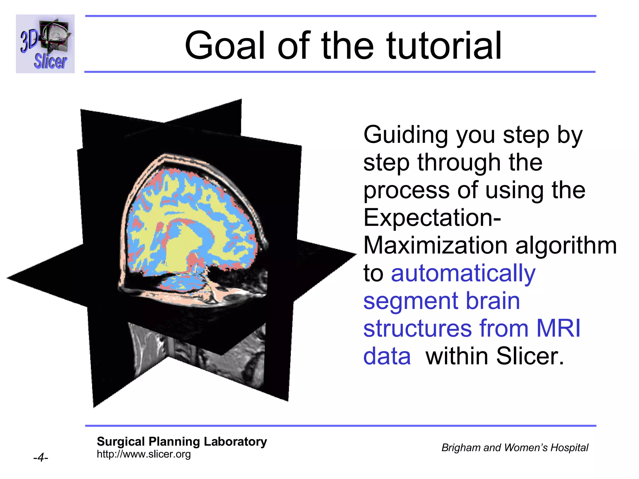
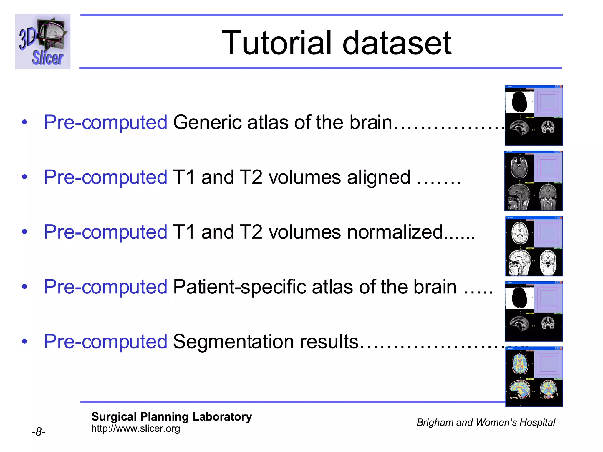
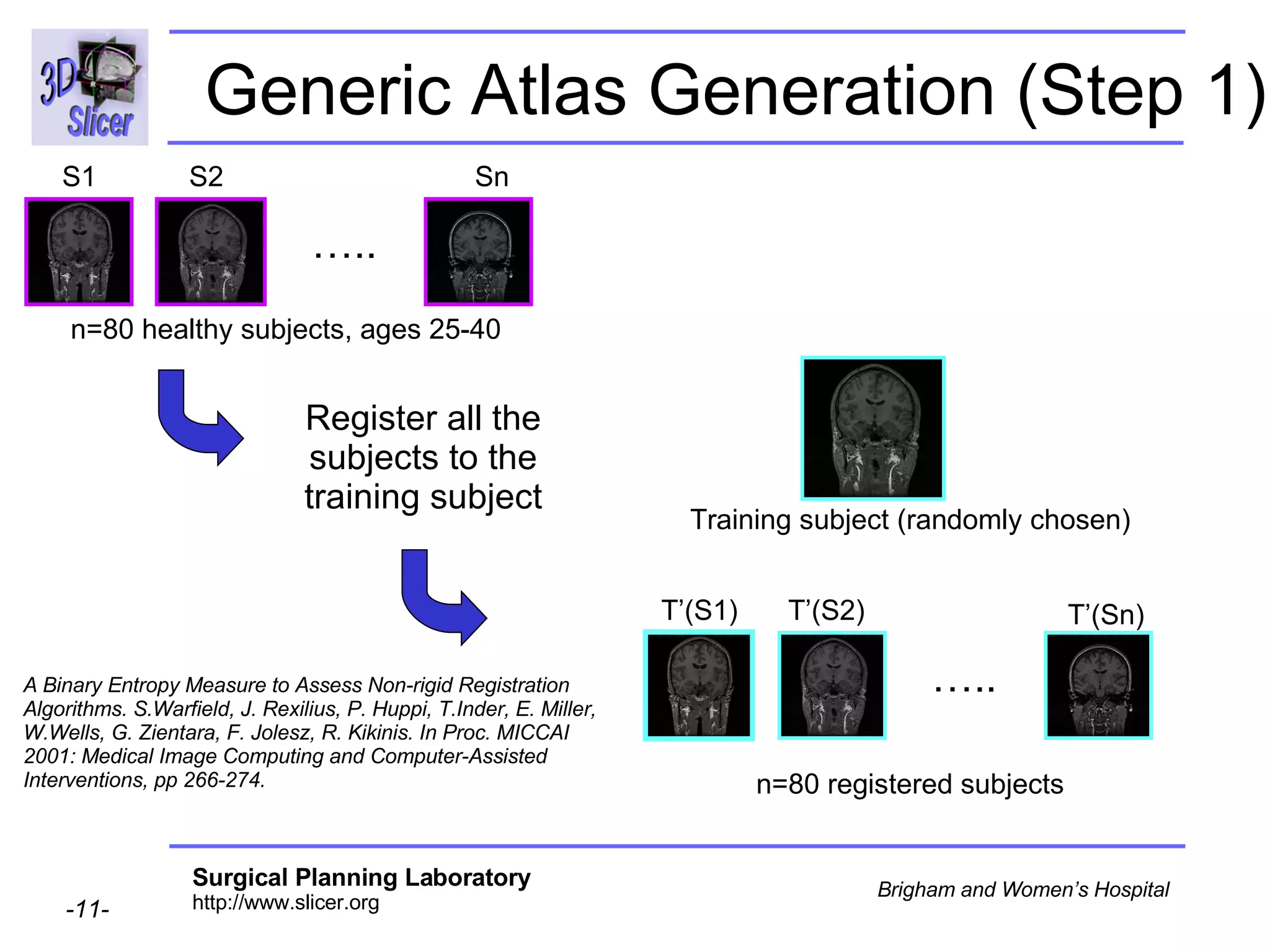
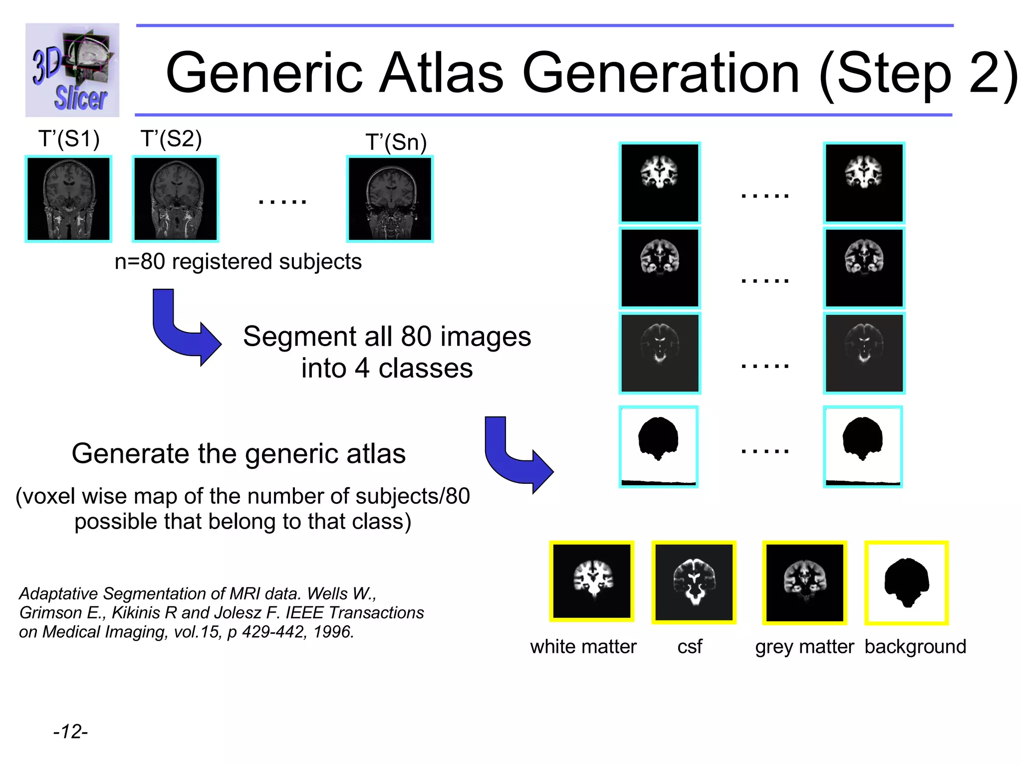
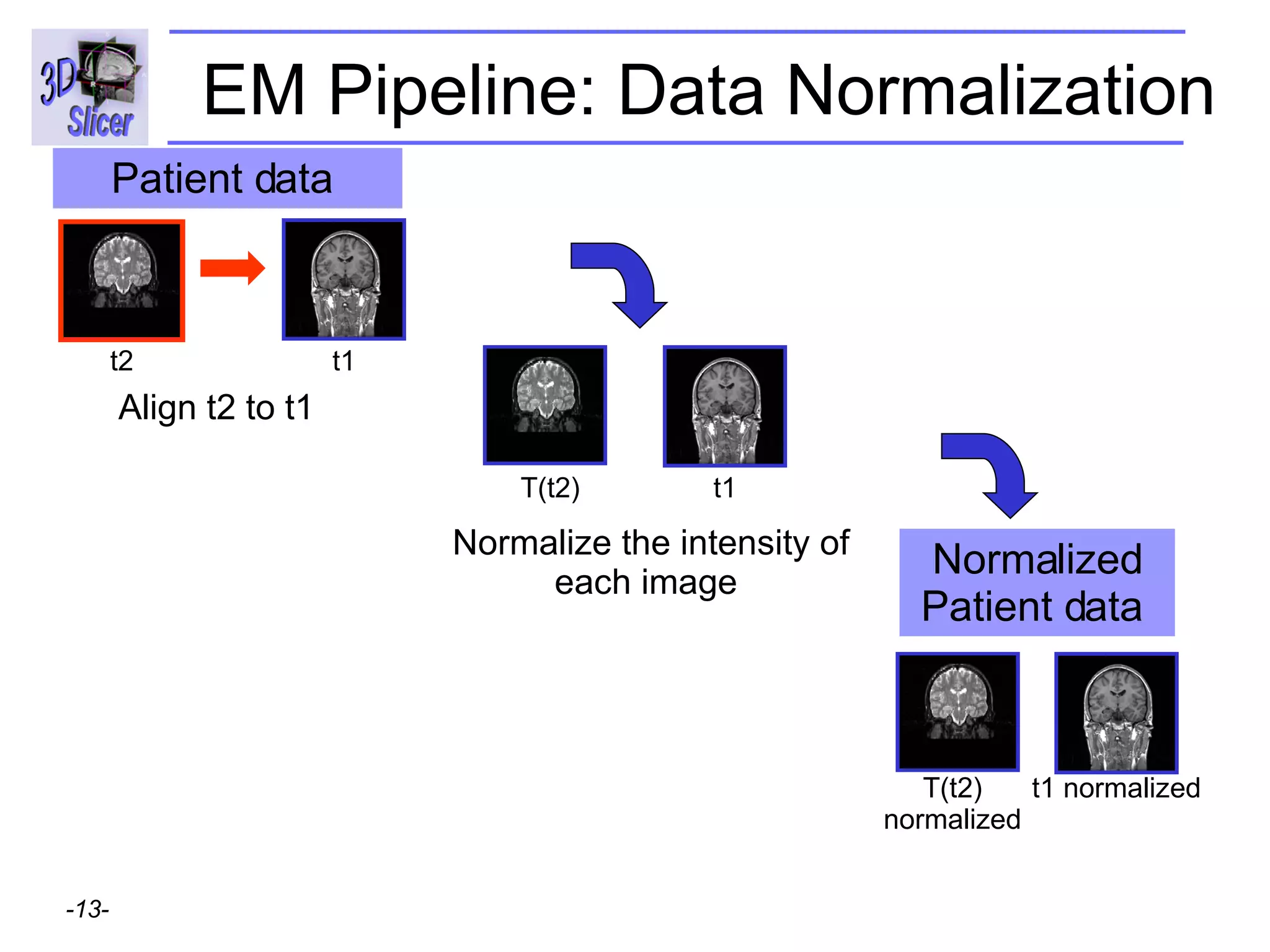
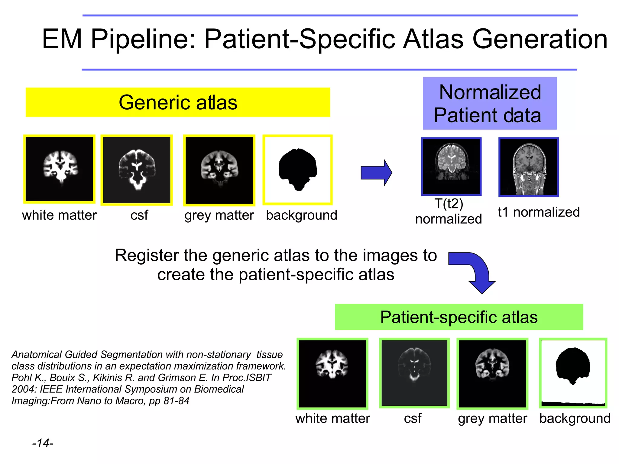
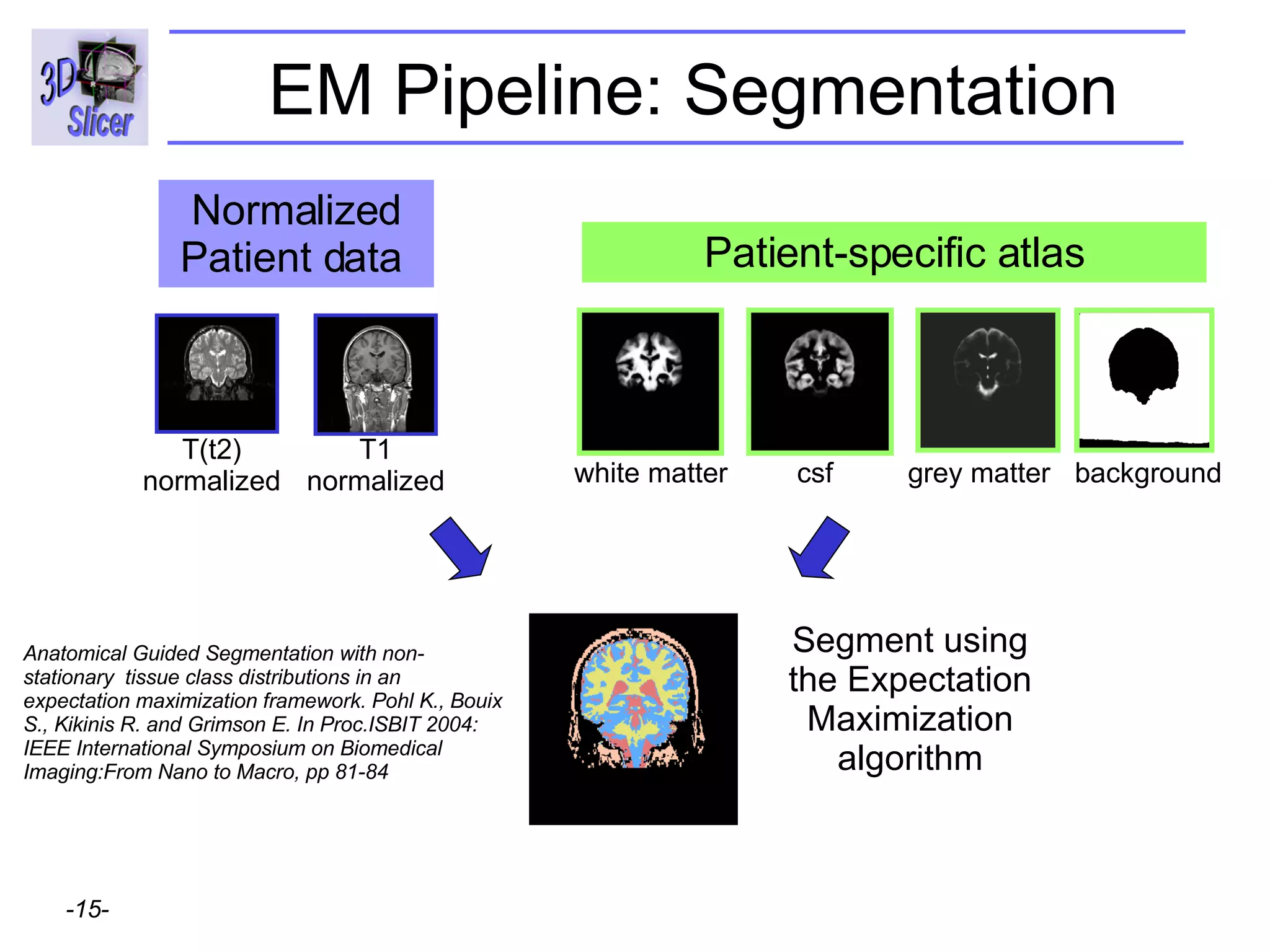
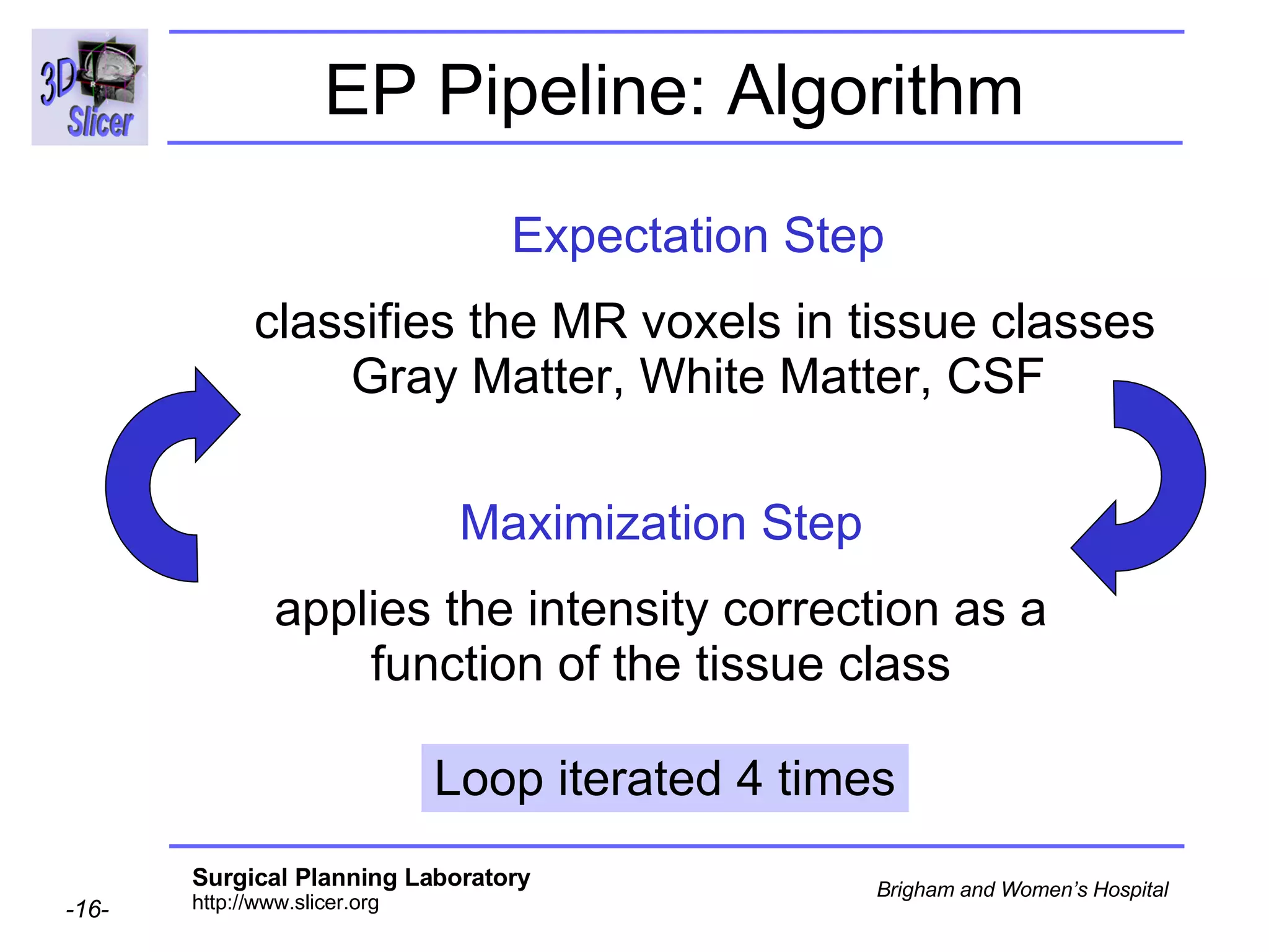
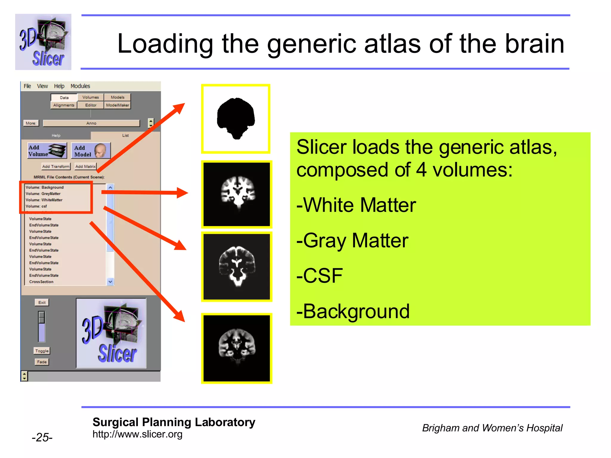
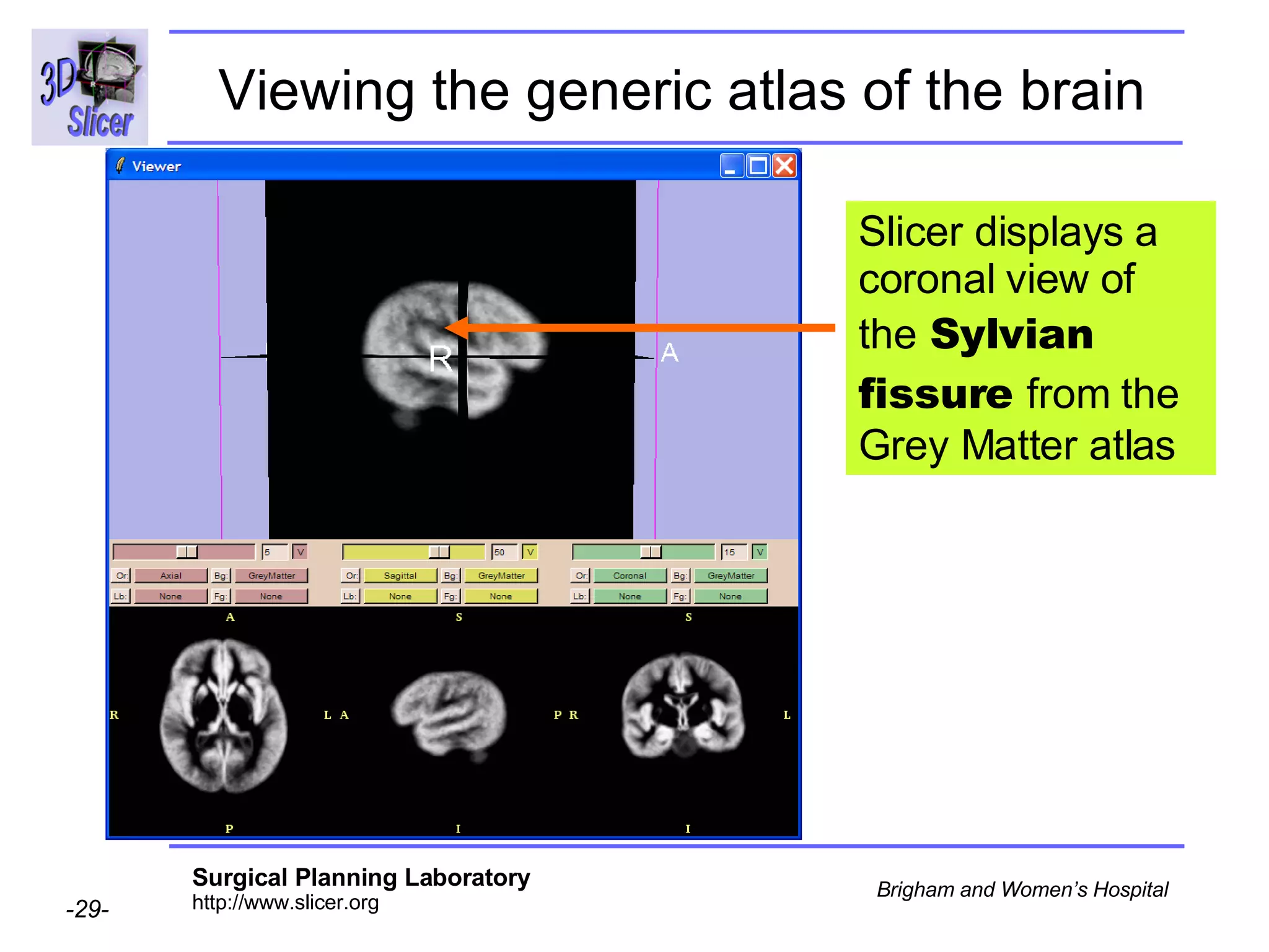
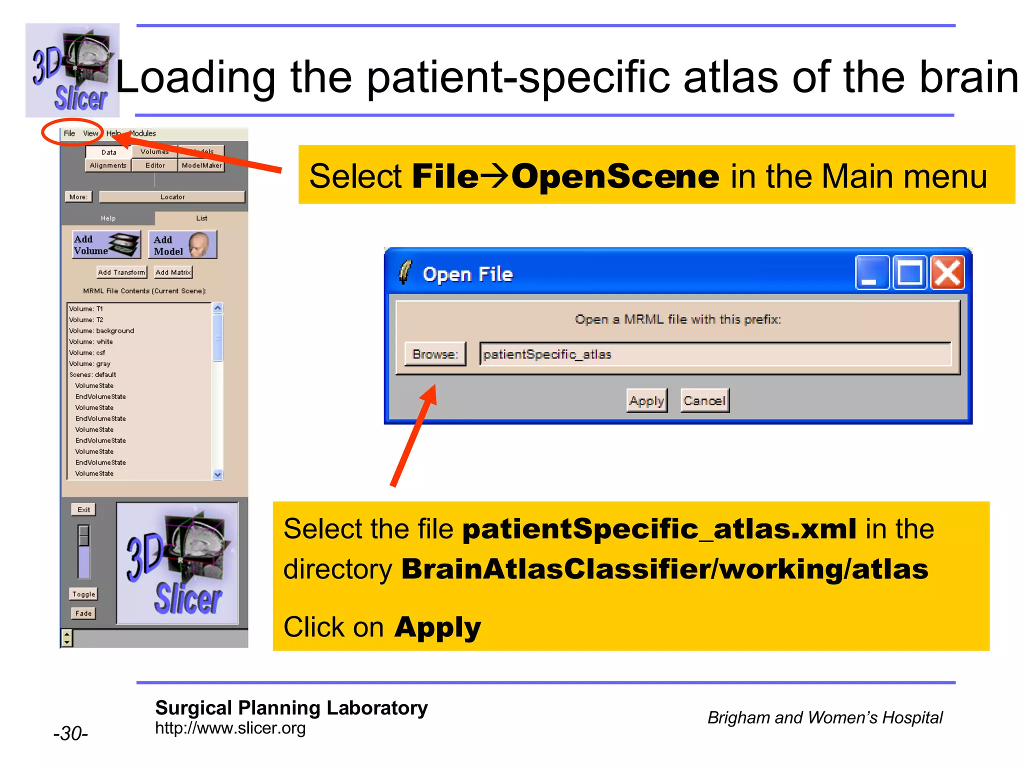
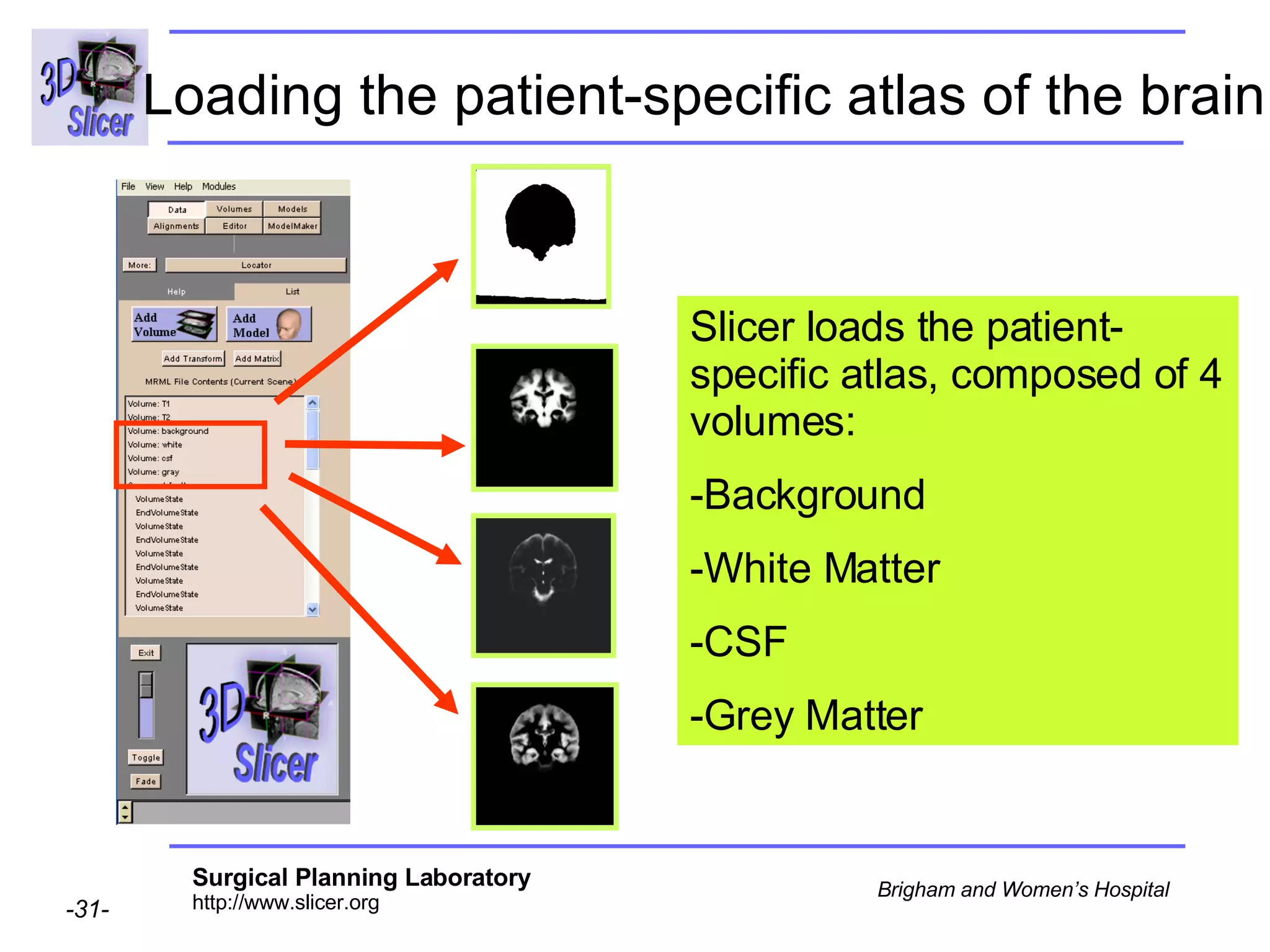
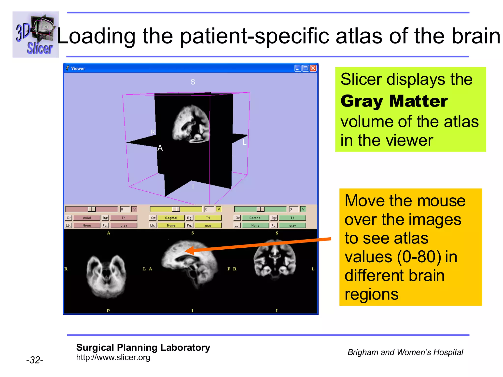
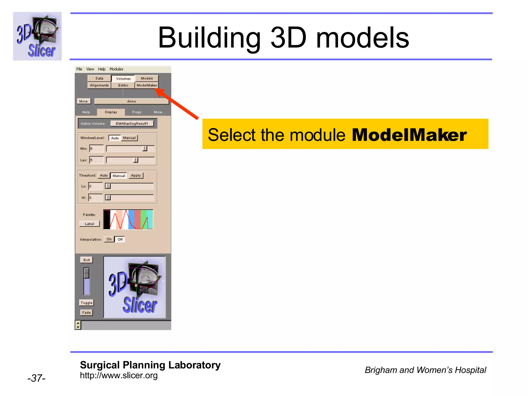
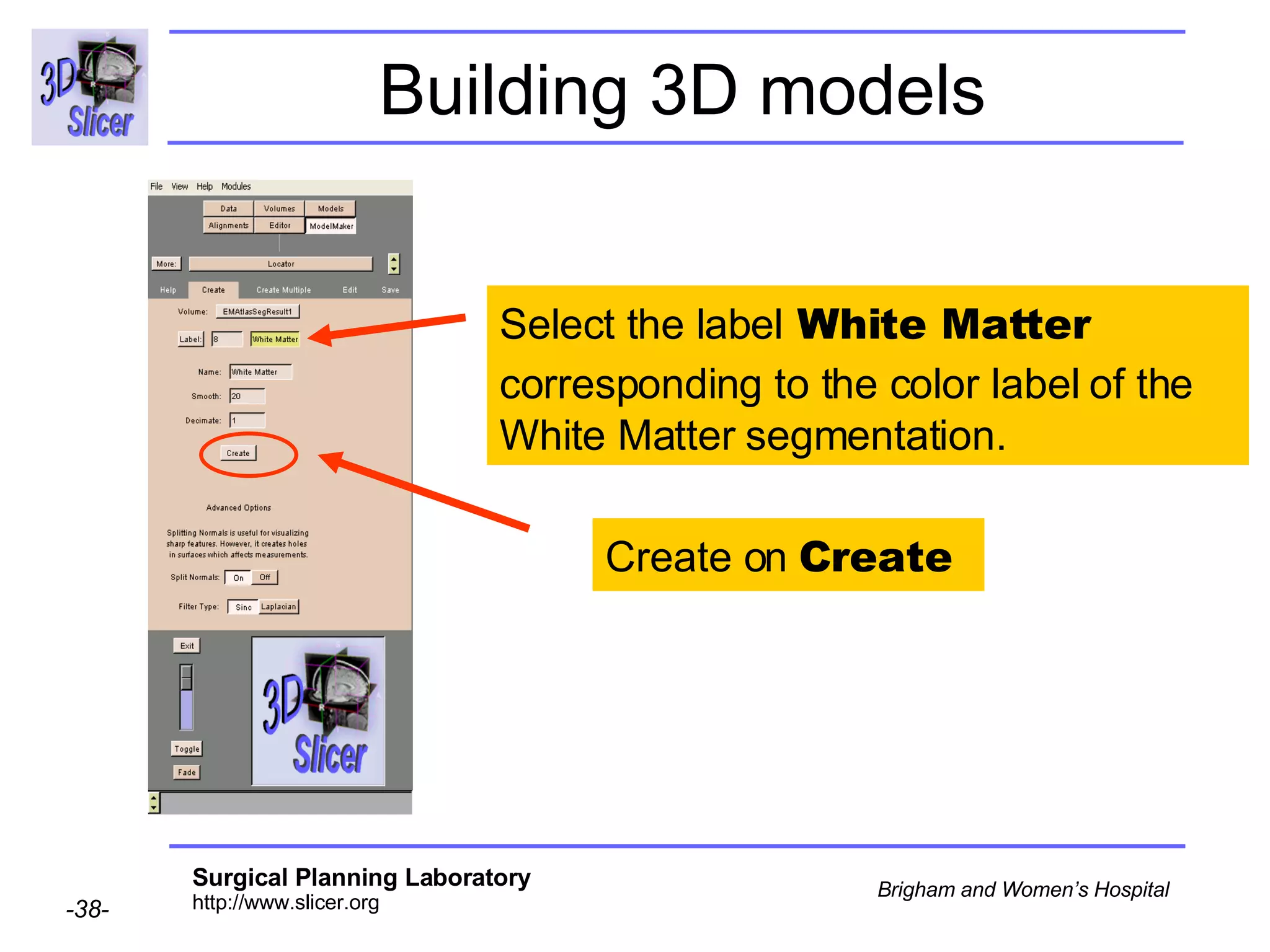
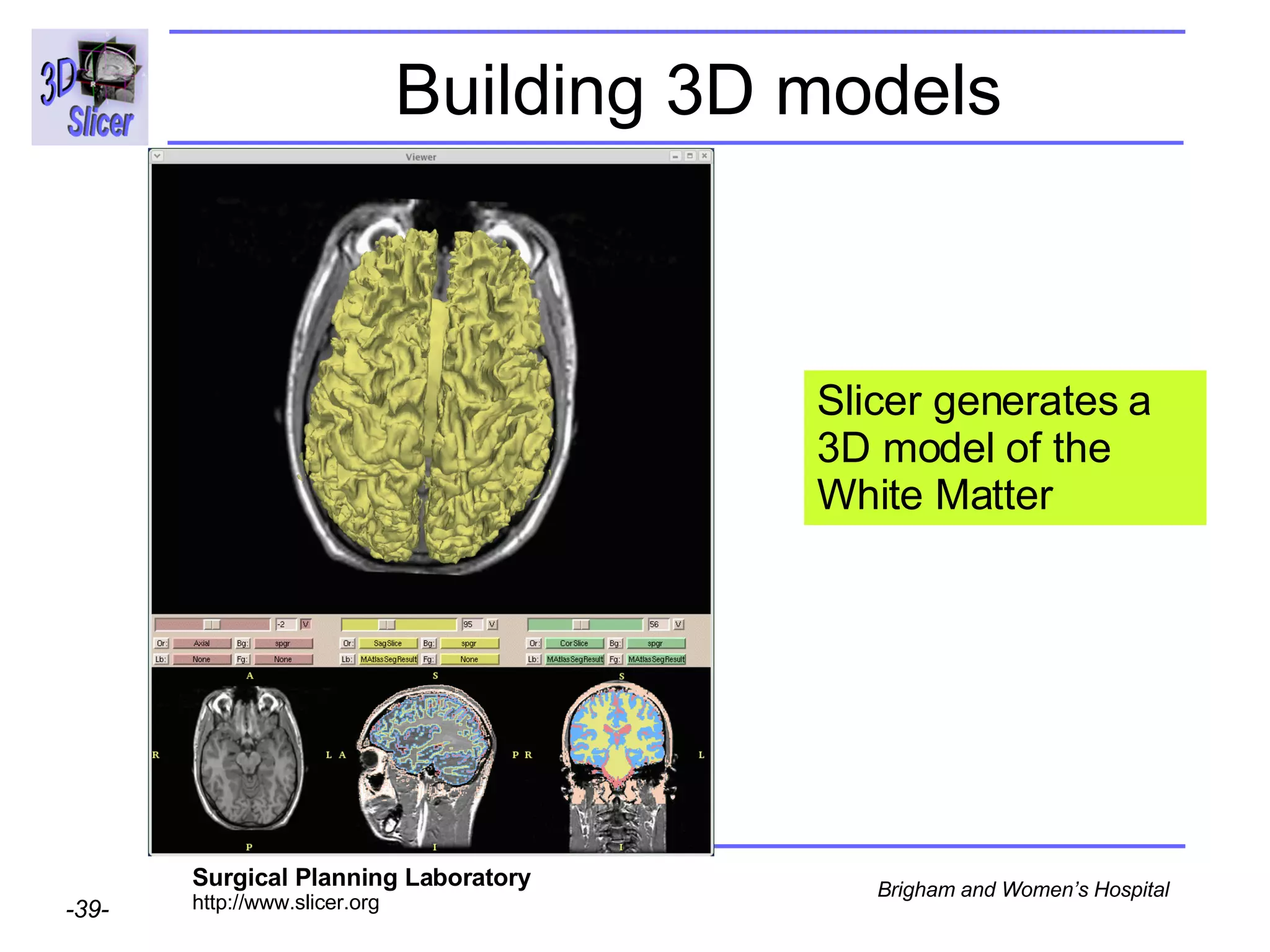
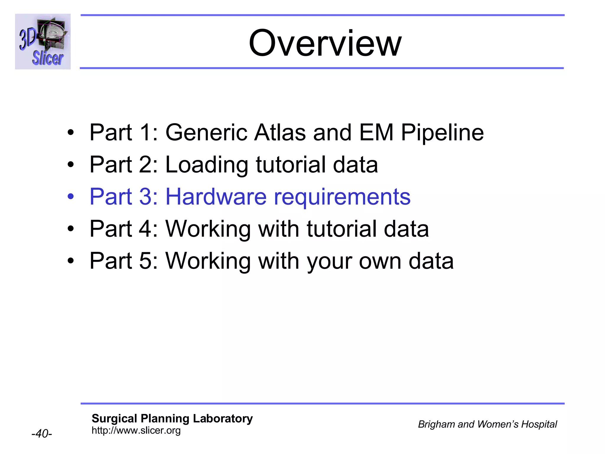
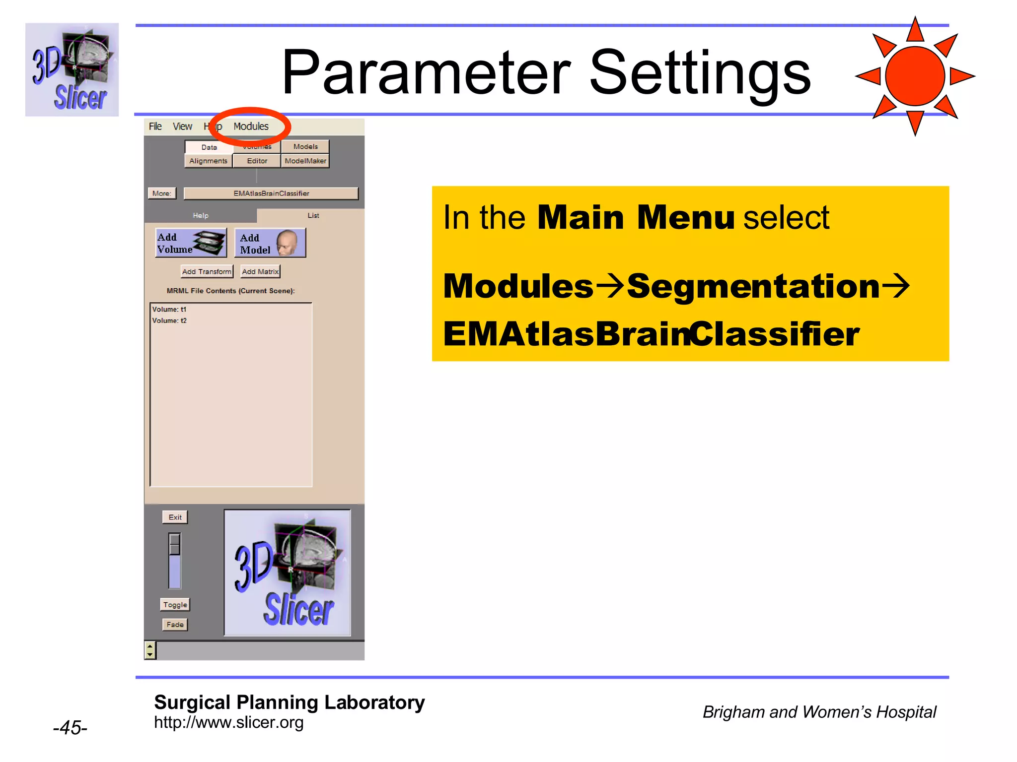
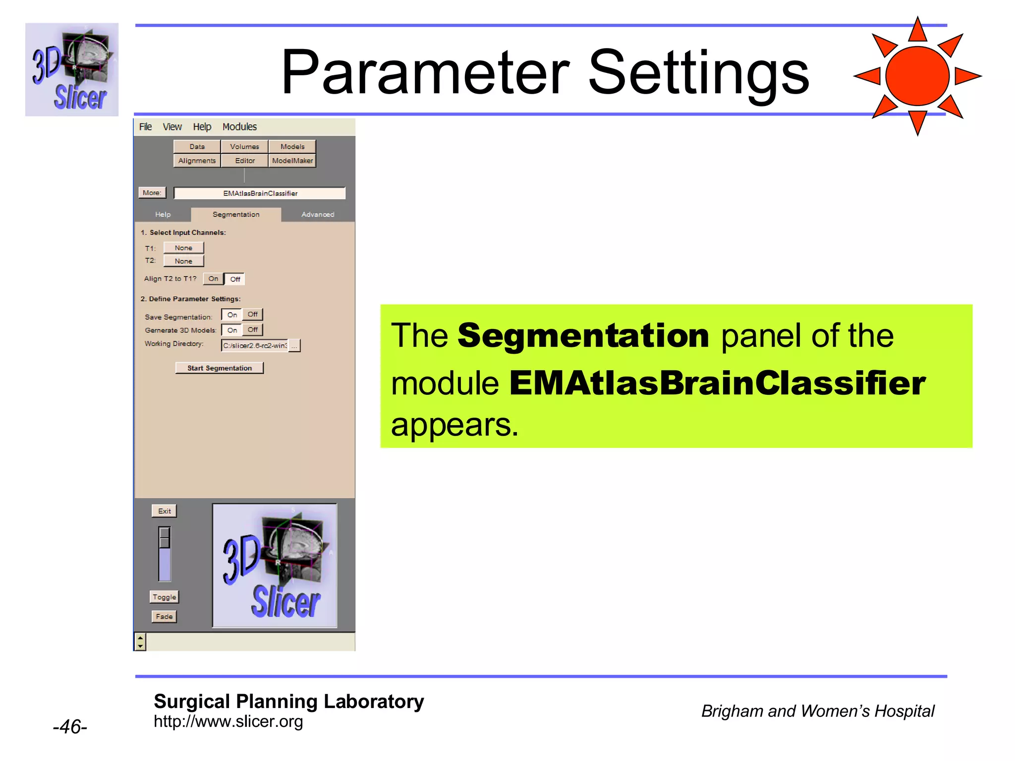
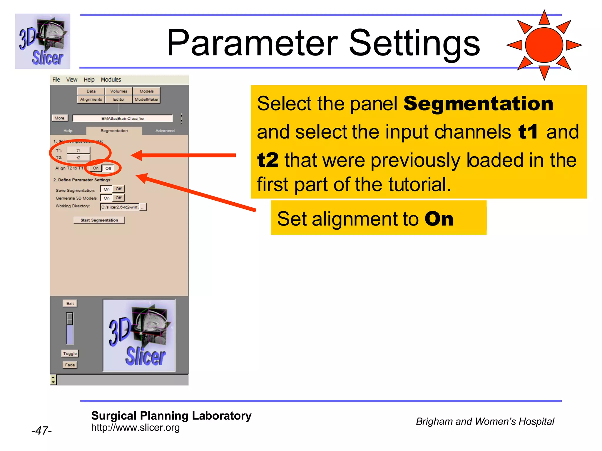
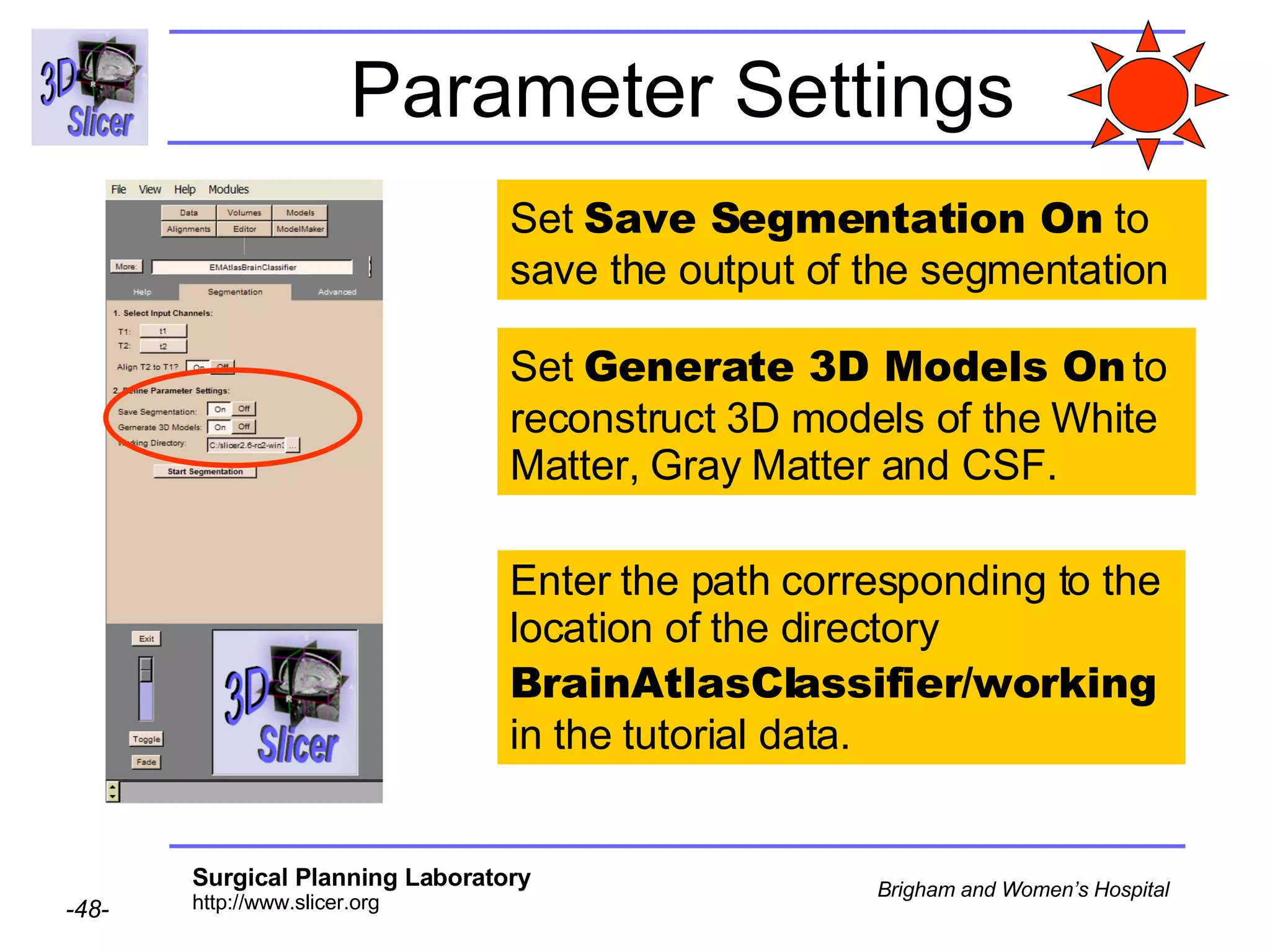
Slicer Training 10  EMAtlasBrainClassifier Sonia Pujol, Ph.D. Randy Gollub, M.D.,Ph.D.
Acknowledgments National Alliance for Medical Image Computing NIH U54EB005149  Neuroimage Analysis Center   NIH P41RR013218  Computer Science and Artificial Intelligence Lab-MIT, Surgical Planning Lab-Harvard Medical School Thanks to Kilian Pohl, Sandy Wells, Martha Shenton, Sylvain Bouix, Alex Guimond, Eric Grimson and Simon Warfield.
Disclaimer It is the responsibility of the user of 3DSlicer to comply with both the terms of the license and with the applicable laws, regulations and rules.
Goal of the tutorial Guiding you step by step through the process of using the Expectation-Maximization algorithm to  automatically segment brain structures from MRI data   within Slicer.
Material Slicer 2.6 www.na-mic.org/Wiki/index.php/Slicer:Slicer2.6_Getting_Started BrainAtlasClassifierTutorial.zip  www.na-mic.org/Wiki/index.php/Slicer:Workshops:User_Training_101 This tutorial assumes that you have already completed Slicer Basics Loading and Viewing Data (Slicer Training 1) and Saving Data ( Slicer Training 7)
Computer Resources The first part of this tutorial teaches you how the module works; it uses  pre-computed  results. The second part guides you through processing the tutorial data yourself with the EMBrainAtlasClassifier module (Slide 40).  For this part, your computer must have adequate processing speed and RAM.  The final part shows you how to run this module on your own data (Slide 51).
EMBrainAtlasClassifier
Pre-computed  Generic atlas of the brain…………………. Pre-computed  T1 and T2 volumes aligned ……. Pre-computed  T1 and T2 volumes normalized...... Pre-computed  Patient-specific atlas of the brain …..  Pre-computed  Segmentation results…………………….. Tutorial dataset
Overview Part 1: Generic Atlas and EM Pipeline   Part 2: Loading tutorial data Part 3: Hardware requirements Part 4: Working with tutorial data Part 5: Working with your own data
Generic Atlas and EM Pipeline  This module relies on a previously computed generic atlas. Running the EM segmentation requires that you have  installed the generic atlas  and that your target datasets go through a  processing pipeline.
Generic Atlas Generation (Step 1) Register all the subjects to the training subject … .. S1 S2 Sn n=80 healthy subjects, ages 25-40 Training subject (randomly chosen) … .. T’(S1) T’(S2) T’(Sn) n=80 registered subjects A Binary Entropy Measure to Assess Non-rigid Registration Algorithms. S.Warfield, J. Rexilius, P. Huppi, T.Inder, E. Miller, W.Wells, G. Zientara, F. Jolesz, R. Kikinis. In Proc. MICCAI 2001: Medical Image Computing and Computer-Assisted Interventions, pp 266-274.
Segment all 80 images into 4 classes … .. T’(S1) T’(S2) T’(Sn) n=80 registered subjects … .. … .. … .. … .. Generate the generic atlas  (voxel wise map of the number of subjects/80 possible that belong to that class) Adaptative Segmentation of MRI data. Wells W., Grimson E., Kikinis R and Jolesz F. IEEE Transactions on Medical Imaging, vol.15, p 429-442, 1996. Generic Atlas Generation (Step 2) white matter csf grey matter background
EM Pipeline: Data Normalization Align t2 to t1 Normalize the intensity of each image  t2 t1 Patient data  Normalized Patient data  t1 T(t2) t1 normalized T(t2) normalized
EM Pipeline: Patient-Specific Atlas Generation Register the generic atlas to the images to create the patient-specific atlas white matter csf grey matter background Generic atlas Anatomical Guided Segmentation with non-stationary  tissue class distributions in an expectation maximization framework. Pohl K., Bouix S., Kikinis R. and Grimson E. In Proc.ISBIT 2004: IEEE International Symposium on Biomedical Imaging:From Nano to Macro, pp 81-84 Patient-specific atlas white matter csf grey matter background Normalized Patient data  t1 normalized T(t2) normalized
EM Pipeline: Segmentation Patient-specific atlas white matter csf grey matter background Segment using the Expectation Maximization algorithm Normalized Patient data  Anatomical Guided Segmentation with non-stationary  tissue class distributions in an expectation maximization framework. Pohl K., Bouix S., Kikinis R. and Grimson E. In Proc.ISBIT 2004: IEEE International Symposium on Biomedical Imaging:From Nano to Macro, pp 81-84 T1 normalized T(t2) normalized
EP Pipeline: Algorithm   Maximization Step applies the intensity correction as a function of the tissue class Expectation Step classifies the MR voxels in tissue classes Gray Matter, White Matter, CSF Loop iterated 4 times
Overview Part 1: Generic Atlas and EM Pipeline Part 2: Loading tutorial data Part 3: Hardware requirements Part 4: Working with tutorial data Part 5: Working with your own data
Loading T1 volume Click  Add Volume  in the Panel  Data
Loading T1 volume Load the volume  t1  from the directory named  /BrainAtlasClassifier/data Click  Add Volume  and select  Basic  in the Panel  Props  of the module Volumes Click on Apply
Loading T1 volume Slicer loads the volume  t1  in the viewer.
Loading T2 volume Click on Image Headers  Manual Click  Add Volume  and select  Basic  in the Panel  Props  of the module Volumes Select the volume  t2 Click on  Apply
Loading T2 volume The tutorial dataset t2 was acquired in the Coronal Posterior-Anterior orientation. Select the Scan order  Coronal:PA Click on  Apply
Loading T2 volume Slicer loads the volume  t2  in the viewer.
Loading the generic atlas of the brain   Select  File  OpenScene  in the Main menu. Select the file  generic_atlas.xml  in the directory  BrainAtlasClassifier/atlas Click on  Apply
Loading the generic atlas of the brain Slicer loads the generic atlas, composed of 4 volumes:  White Matter  Gray Matter  CSF Background
Viewing the generic atlas of the brain   Move the mouse over the images to see atlas values (0-80) in different brain regions Slicer displays the generic atlas of the brain in the viewer.
Loading the generic atlas of the brain   Left click on  Bg  to step through viewing each component.
Viewing the generic atlas of the brain   In the  Control Panel  left-click on  Views  and select the view  Sylvian Fissure
Viewing the generic atlas of the brain Slicer displays a coronal view of the  Sylvian fissure  from the Grey Matter atlas
Loading the patient-specific atlas of the brain   Select  File  OpenScene  in the Main menu Select the file  patientSpecific_atlas.xml  in the directory  BrainAtlasClassifier/working/atlas Click on  Apply
Loading the patient-specific atlas of the brain   Slicer loads the patient-specific atlas, composed of 4 volumes:  Background  White Matter CSF  Grey Matter
Loading the patient-specific atlas of the brain Slicer displays the  Gray Matter  volume of the atlas in the viewer Move the mouse over the images to see atlas values (0-80) in different brain regions
Loading the Segmentation results Select  File  OpenScene  in the Main menu. Select the file  segmentation  in the directory  BrainAtlasClassifier/working/EMSegmentation   and click on  Apply
Loading the Segmentation results Slicer superimposes the results of the segmentation on T1 images
Loading the Segmentation results Move the mouse over the images in the 2D Viewer Slicer displays the names of the labels corresponding to the segmented structures:  - White Matter (yellow)  Grey Matter  (blue) CSF (red)  Background (pink)
Building 3D models Double-click on the volume  Volume:EMBrainSegResult1
Building 3D models Select the module  ModelMaker
Building 3D models Select the label  White Matter  corresponding to the color label of the   White Matter segmentation. Create on  Create
Building 3D models Slicer generates a 3D model of the White Matter
Overview Part 1: Generic Atlas and EM Pipeline  Part 2: Loading tutorial data Part 3: Hardware requirements Part 4: Working with tutorial data Part 5: Working with your own data
Hardware: constraints Minimal requirements RAM: 1 GB Processor: 2 GHz Segmentation algorithm is computationally demanding.
Module Performance Examples of processing time for the  EMBrainAtlasClassifier Sun Solaris 12 UltraSparc-III processors   10 GB RAM:  55 min Debian Pentium 4-M CPU 2.4 GHz, 2 GB RAM :  45 min  RedHat 64 bit 4 Gig  2x 3.0  GHz Xeon Processor:  40 min
Overview Part 1: Generic Atlas and EM Pipeline Part 2: Loading tutorial data Part 3: Hardware requirements Part 4: Working with tutorial data Part 5: Working with your own data
Implementing the EM algorithm If your  processor meets the requirements  the following steps will guide you through the process of segmenting your data using the EM algorithm  If your processor does not, read through (slide 40) to see what you need to do when you run it on a computer with adequate processing capabilities
Parameter Settings In the  Main Menu  select  Modules  Segmentation   EMAtlasBrainClassifier
Parameter Settings The  Segmentation  panel of the module  EMAtlasBrainClassifier  appears.
Parameter Settings Select the panel  Segmentation  and select the input channels  t1  and  t2  that were previously loaded in the first part of the tutorial. Set alignment to  On
Parameter Settings Set  Save Segmentation On  to save the output of the segmentation Enter the path corresponding to the location of the directory  BrainAtlasClassifier/working  in the tutorial data. Set  Generate 3D Models On  to reconstruct 3D models of the White Matter, Gray Matter and CSF.
Automatic Segmentation Click on  Start   Segmentation Expected mean processing time reminder :  45 min
Atlas loading The program looks for a generic atlas at the default location  Modules/vtkEMBrainAtlasClassifier
Atlas loading A message inviting you to download the generic atlas from the web appears. Click  OK.  This message will happen   only once   after having installed Slicer.
Atlas loading (automatic) Slicer downloads the atlas from the web. Click  OK  once the installation is completed.
Atlas loading (manual) If you experience problems with the automatic atlas loading,  manually  download the atlas from the links stated below: Unix/Linux/Mac:  http://na-mic.org/Wiki/images/8/8d/VtkEMAtlasBrainClassifier_AtlasDefault.tar.gz Windows: http://na-mic.org/Wiki/images/5/57/VtkEMAtlasBrainClassifier_AtlasDefault.zip
Atlas installation Manually unzip the archive of the atlas in the directory  Modules/vtkEMAtlasBrainClassifier/atlas
Atlas installation  (Non-Windows Users) Check that the atlas is located in the directory Modules/vtkEMAtlasBrainClassifier /atlas
Atlas installation (additional step only required for  Windows Users) Built-in Windows unzip wizard adds an extra level of directory  Modules/vtkEMAtlasBrainClassifier /atlas/atlas   Move the atlas data one level-up to the correct directory  Modules/vtkEMAtlasBrainClassifier /atlas and delete the unnecessary directory
Overview Part 1: Generic Atlas and EM Pipeline Part 2: Loading tutorial data Part 3: Hardware requirements Part 4: Working with tutorial data Part 5: Working with your own data
Data Acquisition: Tutorial data The  tutorial dataset  was acquired with the following parameters T1 volume: Coronal series of contiguous Spoiled Gradient (SPGR) images (124 slices of 1.5 mm thickness, voxel dimensions 0.9375 x 0.9375 x 1.5 mm)  T2 volume: Axial series of contiguous double-echo images (Proton Density and T2 Weighted, 108 slices of 3 mm slice thickness, voxel dimensions 0.9375 x 0.9375 x 3 mm) isotropic t2  Dimension 0.9375mm x 0.9375mm x 3mm  More details can be found on the NA-MIC wiki http://www.na-mic.org/Wiki/index.php/Brockton_MRI_Scan_Parameters
Data Acquisition: your data You’ll need to experiment the EMBrainAtlasClassifier module with your own data. We suggest  High resolution T1 and T2 weighted images .
Working with your own data Load T1 and T2 as  Input Channels, and set  Align T2 to T1   On  to register  the two volumes.
Working with your own data Set  Save Segmentation On  to save the output of the segmentation Enter the path corresponding to the working directory for your own data Set  Generate 3D Models On  to reconstruct 3D models of the White Matter, Gray Matter and CSF. Click on  Start Segmentation
Conclusion Automatic segmentation of MRI brain data in White Matter, Grey Matter and Cerebrospinal Fluid. Open-source environment

Automatic Brain Segmentation-3770

  • 1.
    Slicer Training 10 EMAtlasBrainClassifier Sonia Pujol, Ph.D. Randy Gollub, M.D.,Ph.D.
  • 2.
    Acknowledgments National Alliancefor Medical Image Computing NIH U54EB005149 Neuroimage Analysis Center NIH P41RR013218 Computer Science and Artificial Intelligence Lab-MIT, Surgical Planning Lab-Harvard Medical School Thanks to Kilian Pohl, Sandy Wells, Martha Shenton, Sylvain Bouix, Alex Guimond, Eric Grimson and Simon Warfield.
  • 3.
    Disclaimer It isthe responsibility of the user of 3DSlicer to comply with both the terms of the license and with the applicable laws, regulations and rules.
  • 4.
    Goal of thetutorial Guiding you step by step through the process of using the Expectation-Maximization algorithm to automatically segment brain structures from MRI data within Slicer.
  • 5.
    Material Slicer 2.6www.na-mic.org/Wiki/index.php/Slicer:Slicer2.6_Getting_Started BrainAtlasClassifierTutorial.zip www.na-mic.org/Wiki/index.php/Slicer:Workshops:User_Training_101 This tutorial assumes that you have already completed Slicer Basics Loading and Viewing Data (Slicer Training 1) and Saving Data ( Slicer Training 7)
  • 6.
    Computer Resources Thefirst part of this tutorial teaches you how the module works; it uses pre-computed results. The second part guides you through processing the tutorial data yourself with the EMBrainAtlasClassifier module (Slide 40). For this part, your computer must have adequate processing speed and RAM. The final part shows you how to run this module on your own data (Slide 51).
  • 7.
  • 8.
    Pre-computed Genericatlas of the brain…………………. Pre-computed T1 and T2 volumes aligned ……. Pre-computed T1 and T2 volumes normalized...... Pre-computed Patient-specific atlas of the brain ….. Pre-computed Segmentation results…………………….. Tutorial dataset
  • 9.
    Overview Part 1:Generic Atlas and EM Pipeline Part 2: Loading tutorial data Part 3: Hardware requirements Part 4: Working with tutorial data Part 5: Working with your own data
  • 10.
    Generic Atlas andEM Pipeline This module relies on a previously computed generic atlas. Running the EM segmentation requires that you have installed the generic atlas and that your target datasets go through a processing pipeline.
  • 11.
    Generic Atlas Generation(Step 1) Register all the subjects to the training subject … .. S1 S2 Sn n=80 healthy subjects, ages 25-40 Training subject (randomly chosen) … .. T’(S1) T’(S2) T’(Sn) n=80 registered subjects A Binary Entropy Measure to Assess Non-rigid Registration Algorithms. S.Warfield, J. Rexilius, P. Huppi, T.Inder, E. Miller, W.Wells, G. Zientara, F. Jolesz, R. Kikinis. In Proc. MICCAI 2001: Medical Image Computing and Computer-Assisted Interventions, pp 266-274.
  • 12.
    Segment all 80images into 4 classes … .. T’(S1) T’(S2) T’(Sn) n=80 registered subjects … .. … .. … .. … .. Generate the generic atlas (voxel wise map of the number of subjects/80 possible that belong to that class) Adaptative Segmentation of MRI data. Wells W., Grimson E., Kikinis R and Jolesz F. IEEE Transactions on Medical Imaging, vol.15, p 429-442, 1996. Generic Atlas Generation (Step 2) white matter csf grey matter background
  • 13.
    EM Pipeline: DataNormalization Align t2 to t1 Normalize the intensity of each image t2 t1 Patient data Normalized Patient data t1 T(t2) t1 normalized T(t2) normalized
  • 14.
    EM Pipeline: Patient-SpecificAtlas Generation Register the generic atlas to the images to create the patient-specific atlas white matter csf grey matter background Generic atlas Anatomical Guided Segmentation with non-stationary tissue class distributions in an expectation maximization framework. Pohl K., Bouix S., Kikinis R. and Grimson E. In Proc.ISBIT 2004: IEEE International Symposium on Biomedical Imaging:From Nano to Macro, pp 81-84 Patient-specific atlas white matter csf grey matter background Normalized Patient data t1 normalized T(t2) normalized
  • 15.
    EM Pipeline: SegmentationPatient-specific atlas white matter csf grey matter background Segment using the Expectation Maximization algorithm Normalized Patient data Anatomical Guided Segmentation with non-stationary tissue class distributions in an expectation maximization framework. Pohl K., Bouix S., Kikinis R. and Grimson E. In Proc.ISBIT 2004: IEEE International Symposium on Biomedical Imaging:From Nano to Macro, pp 81-84 T1 normalized T(t2) normalized
  • 16.
    EP Pipeline: Algorithm Maximization Step applies the intensity correction as a function of the tissue class Expectation Step classifies the MR voxels in tissue classes Gray Matter, White Matter, CSF Loop iterated 4 times
  • 17.
    Overview Part 1:Generic Atlas and EM Pipeline Part 2: Loading tutorial data Part 3: Hardware requirements Part 4: Working with tutorial data Part 5: Working with your own data
  • 18.
    Loading T1 volumeClick Add Volume in the Panel Data
  • 19.
    Loading T1 volumeLoad the volume t1 from the directory named /BrainAtlasClassifier/data Click Add Volume and select Basic in the Panel Props of the module Volumes Click on Apply
  • 20.
    Loading T1 volumeSlicer loads the volume t1 in the viewer.
  • 21.
    Loading T2 volumeClick on Image Headers Manual Click Add Volume and select Basic in the Panel Props of the module Volumes Select the volume t2 Click on Apply
  • 22.
    Loading T2 volumeThe tutorial dataset t2 was acquired in the Coronal Posterior-Anterior orientation. Select the Scan order Coronal:PA Click on Apply
  • 23.
    Loading T2 volumeSlicer loads the volume t2 in the viewer.
  • 24.
    Loading the genericatlas of the brain Select File  OpenScene in the Main menu. Select the file generic_atlas.xml in the directory BrainAtlasClassifier/atlas Click on Apply
  • 25.
    Loading the genericatlas of the brain Slicer loads the generic atlas, composed of 4 volumes: White Matter Gray Matter CSF Background
  • 26.
    Viewing the genericatlas of the brain Move the mouse over the images to see atlas values (0-80) in different brain regions Slicer displays the generic atlas of the brain in the viewer.
  • 27.
    Loading the genericatlas of the brain Left click on Bg to step through viewing each component.
  • 28.
    Viewing the genericatlas of the brain In the Control Panel left-click on Views and select the view Sylvian Fissure
  • 29.
    Viewing the genericatlas of the brain Slicer displays a coronal view of the Sylvian fissure from the Grey Matter atlas
  • 30.
    Loading the patient-specificatlas of the brain Select File  OpenScene in the Main menu Select the file patientSpecific_atlas.xml in the directory BrainAtlasClassifier/working/atlas Click on Apply
  • 31.
    Loading the patient-specificatlas of the brain Slicer loads the patient-specific atlas, composed of 4 volumes: Background White Matter CSF Grey Matter
  • 32.
    Loading the patient-specificatlas of the brain Slicer displays the Gray Matter volume of the atlas in the viewer Move the mouse over the images to see atlas values (0-80) in different brain regions
  • 33.
    Loading the Segmentationresults Select File  OpenScene in the Main menu. Select the file segmentation in the directory BrainAtlasClassifier/working/EMSegmentation and click on Apply
  • 34.
    Loading the Segmentationresults Slicer superimposes the results of the segmentation on T1 images
  • 35.
    Loading the Segmentationresults Move the mouse over the images in the 2D Viewer Slicer displays the names of the labels corresponding to the segmented structures: - White Matter (yellow) Grey Matter (blue) CSF (red) Background (pink)
  • 36.
    Building 3D modelsDouble-click on the volume Volume:EMBrainSegResult1
  • 37.
    Building 3D modelsSelect the module ModelMaker
  • 38.
    Building 3D modelsSelect the label White Matter corresponding to the color label of the White Matter segmentation. Create on Create
  • 39.
    Building 3D modelsSlicer generates a 3D model of the White Matter
  • 40.
    Overview Part 1:Generic Atlas and EM Pipeline Part 2: Loading tutorial data Part 3: Hardware requirements Part 4: Working with tutorial data Part 5: Working with your own data
  • 41.
    Hardware: constraints Minimalrequirements RAM: 1 GB Processor: 2 GHz Segmentation algorithm is computationally demanding.
  • 42.
    Module Performance Examplesof processing time for the EMBrainAtlasClassifier Sun Solaris 12 UltraSparc-III processors 10 GB RAM: 55 min Debian Pentium 4-M CPU 2.4 GHz, 2 GB RAM : 45 min RedHat 64 bit 4 Gig 2x 3.0 GHz Xeon Processor: 40 min
  • 43.
    Overview Part 1:Generic Atlas and EM Pipeline Part 2: Loading tutorial data Part 3: Hardware requirements Part 4: Working with tutorial data Part 5: Working with your own data
  • 44.
    Implementing the EMalgorithm If your processor meets the requirements the following steps will guide you through the process of segmenting your data using the EM algorithm If your processor does not, read through (slide 40) to see what you need to do when you run it on a computer with adequate processing capabilities
  • 45.
    Parameter Settings Inthe Main Menu select Modules  Segmentation  EMAtlasBrainClassifier
  • 46.
    Parameter Settings The Segmentation panel of the module EMAtlasBrainClassifier appears.
  • 47.
    Parameter Settings Selectthe panel Segmentation and select the input channels t1 and t2 that were previously loaded in the first part of the tutorial. Set alignment to On
  • 48.
    Parameter Settings Set Save Segmentation On to save the output of the segmentation Enter the path corresponding to the location of the directory BrainAtlasClassifier/working in the tutorial data. Set Generate 3D Models On to reconstruct 3D models of the White Matter, Gray Matter and CSF.
  • 49.
    Automatic Segmentation Clickon Start Segmentation Expected mean processing time reminder : 45 min
  • 50.
    Atlas loading Theprogram looks for a generic atlas at the default location Modules/vtkEMBrainAtlasClassifier
  • 51.
    Atlas loading Amessage inviting you to download the generic atlas from the web appears. Click OK. This message will happen only once after having installed Slicer.
  • 52.
    Atlas loading (automatic)Slicer downloads the atlas from the web. Click OK once the installation is completed.
  • 53.
    Atlas loading (manual)If you experience problems with the automatic atlas loading, manually download the atlas from the links stated below: Unix/Linux/Mac: http://na-mic.org/Wiki/images/8/8d/VtkEMAtlasBrainClassifier_AtlasDefault.tar.gz Windows: http://na-mic.org/Wiki/images/5/57/VtkEMAtlasBrainClassifier_AtlasDefault.zip
  • 54.
    Atlas installation Manuallyunzip the archive of the atlas in the directory Modules/vtkEMAtlasBrainClassifier/atlas
  • 55.
    Atlas installation (Non-Windows Users) Check that the atlas is located in the directory Modules/vtkEMAtlasBrainClassifier /atlas
  • 56.
    Atlas installation (additionalstep only required for Windows Users) Built-in Windows unzip wizard adds an extra level of directory Modules/vtkEMAtlasBrainClassifier /atlas/atlas Move the atlas data one level-up to the correct directory Modules/vtkEMAtlasBrainClassifier /atlas and delete the unnecessary directory
  • 57.
    Overview Part 1:Generic Atlas and EM Pipeline Part 2: Loading tutorial data Part 3: Hardware requirements Part 4: Working with tutorial data Part 5: Working with your own data
  • 58.
    Data Acquisition: Tutorialdata The tutorial dataset was acquired with the following parameters T1 volume: Coronal series of contiguous Spoiled Gradient (SPGR) images (124 slices of 1.5 mm thickness, voxel dimensions 0.9375 x 0.9375 x 1.5 mm) T2 volume: Axial series of contiguous double-echo images (Proton Density and T2 Weighted, 108 slices of 3 mm slice thickness, voxel dimensions 0.9375 x 0.9375 x 3 mm) isotropic t2 Dimension 0.9375mm x 0.9375mm x 3mm More details can be found on the NA-MIC wiki http://www.na-mic.org/Wiki/index.php/Brockton_MRI_Scan_Parameters
  • 59.
    Data Acquisition: yourdata You’ll need to experiment the EMBrainAtlasClassifier module with your own data. We suggest High resolution T1 and T2 weighted images .
  • 60.
    Working with yourown data Load T1 and T2 as Input Channels, and set Align T2 to T1 On to register the two volumes.
  • 61.
    Working with yourown data Set Save Segmentation On to save the output of the segmentation Enter the path corresponding to the working directory for your own data Set Generate 3D Models On to reconstruct 3D models of the White Matter, Gray Matter and CSF. Click on Start Segmentation
  • 62.
    Conclusion Automatic segmentationof MRI brain data in White Matter, Grey Matter and Cerebrospinal Fluid. Open-source environment