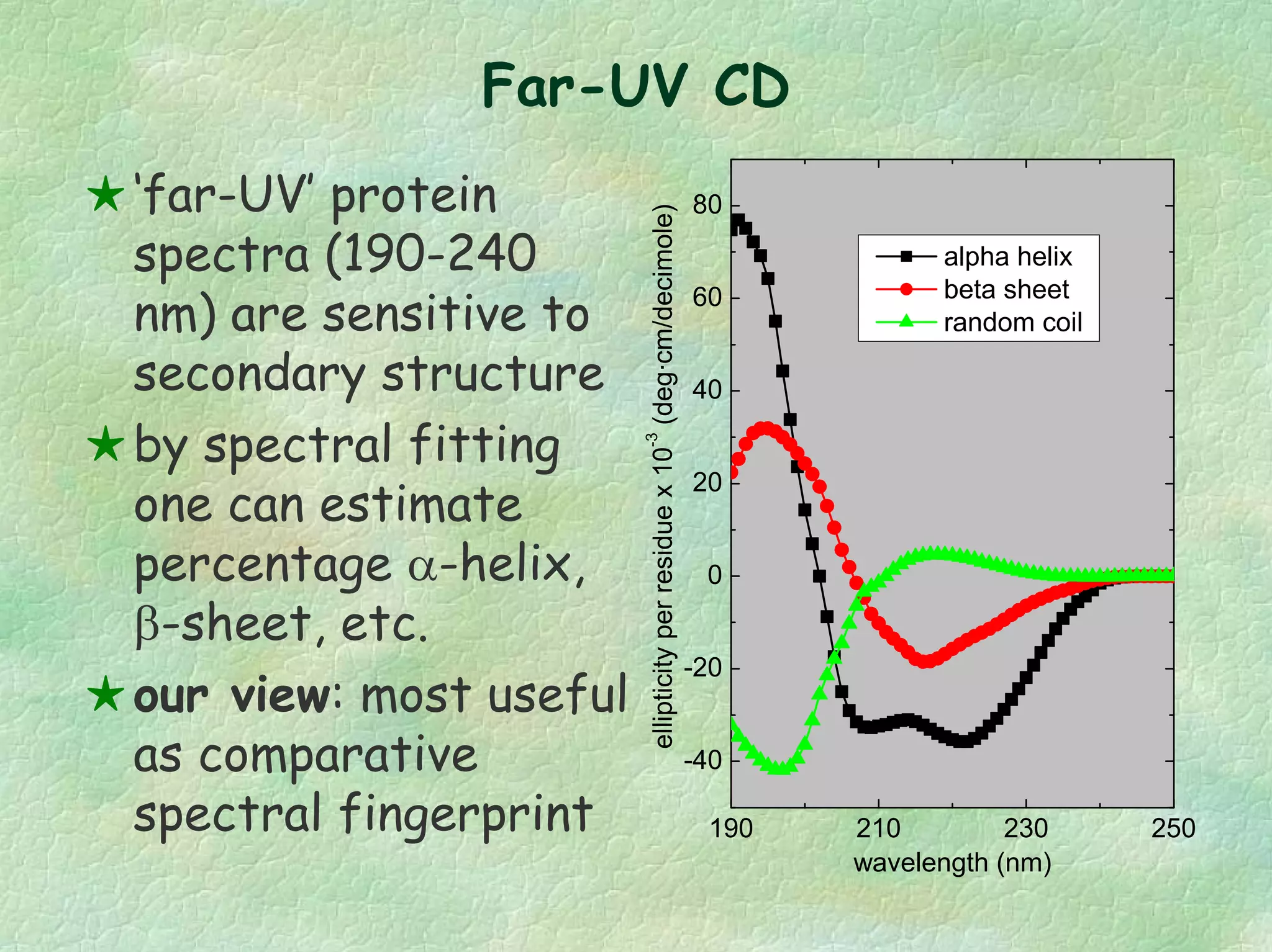
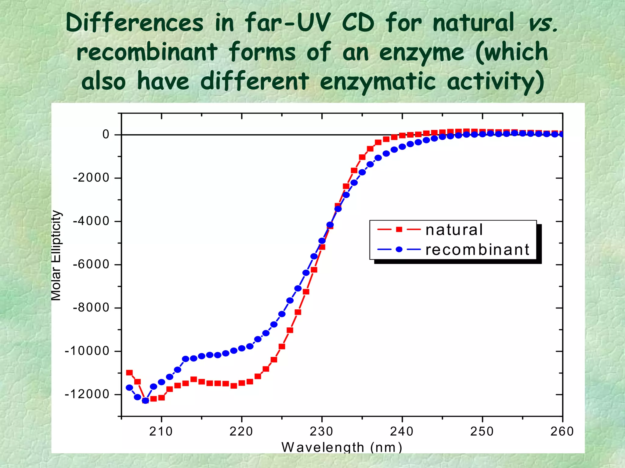
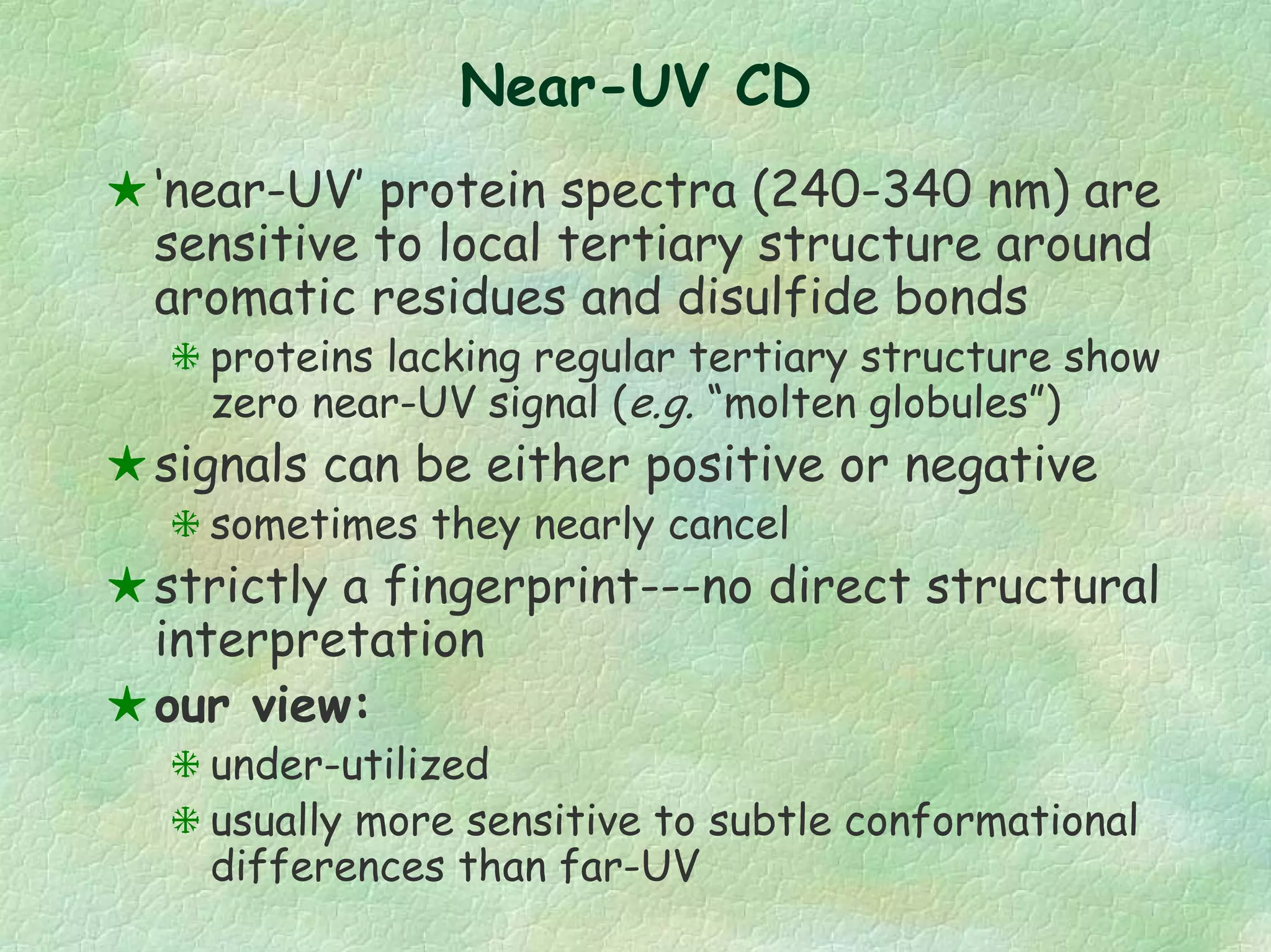
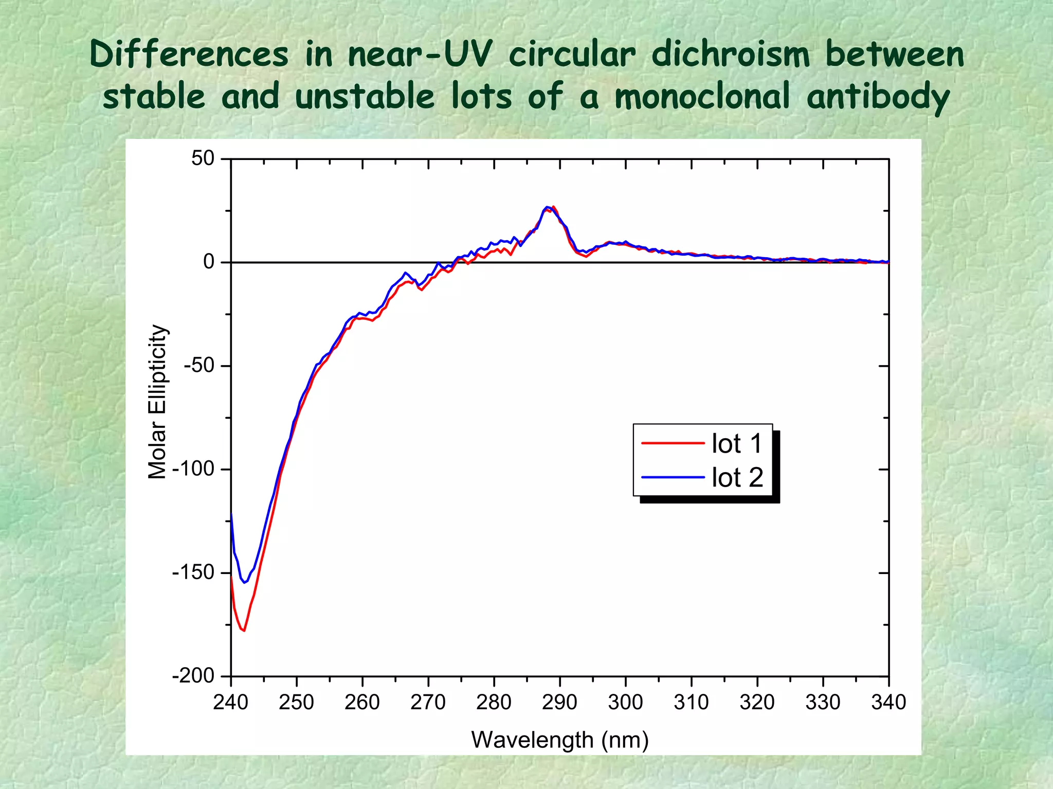
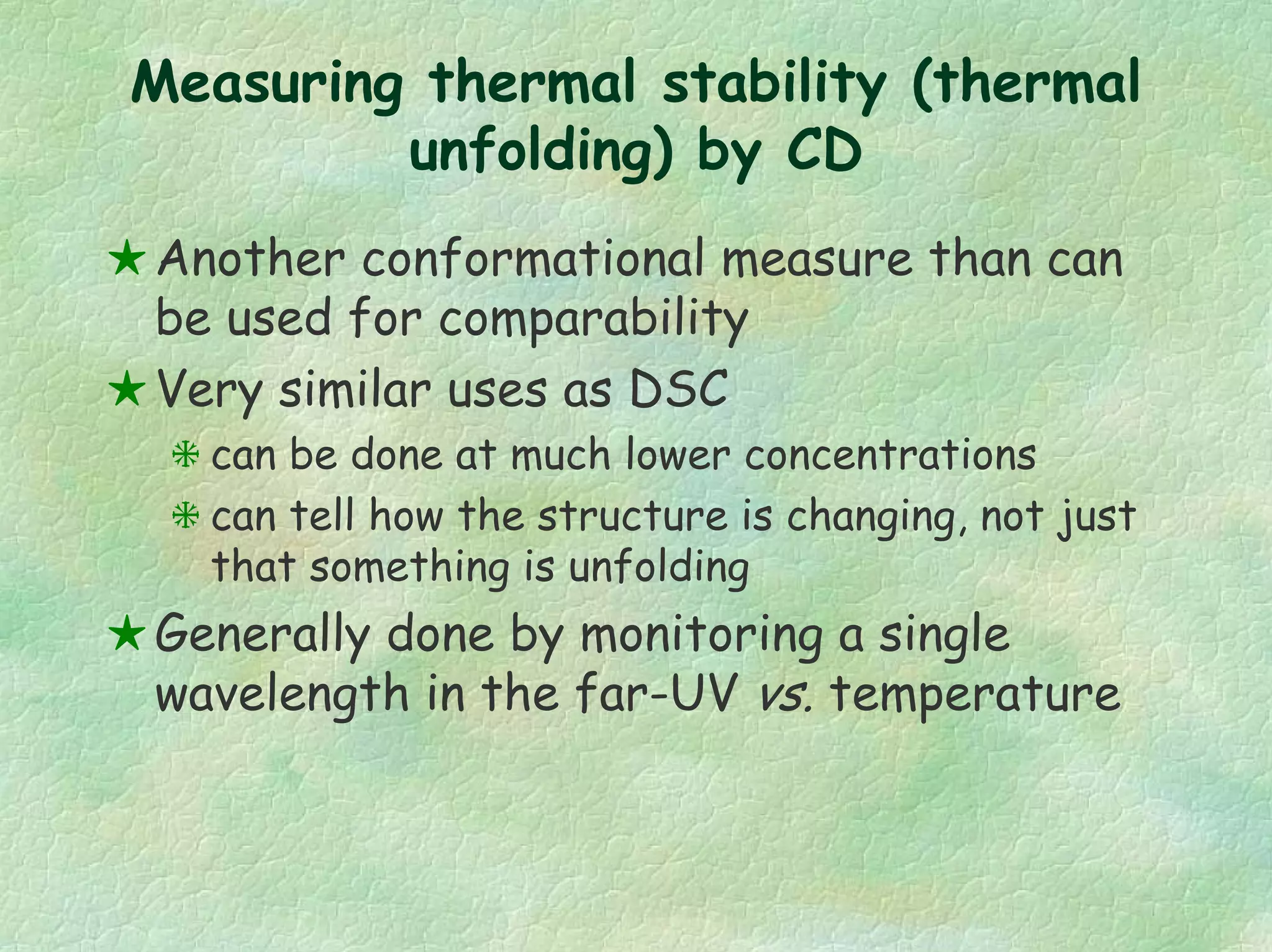
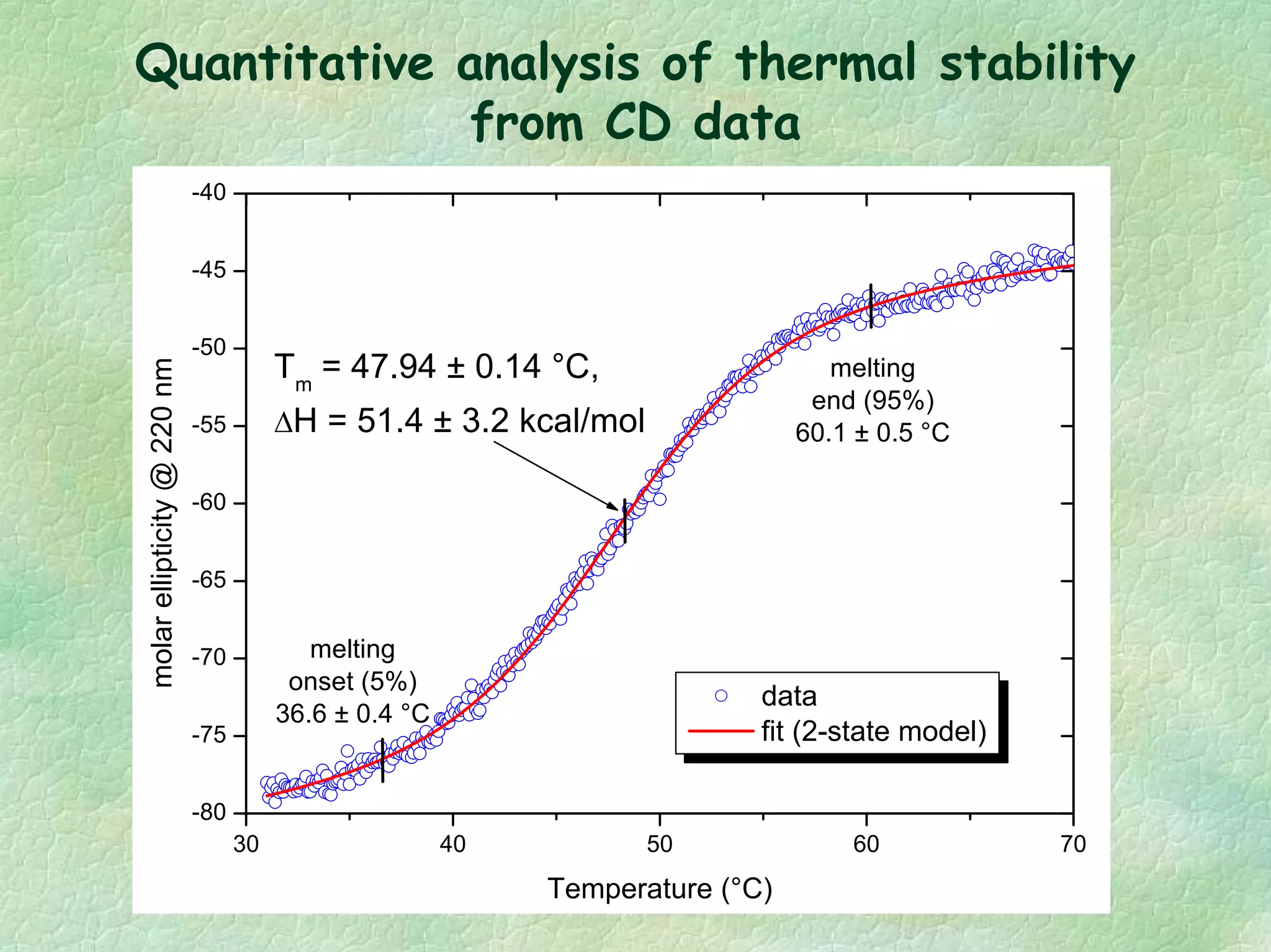
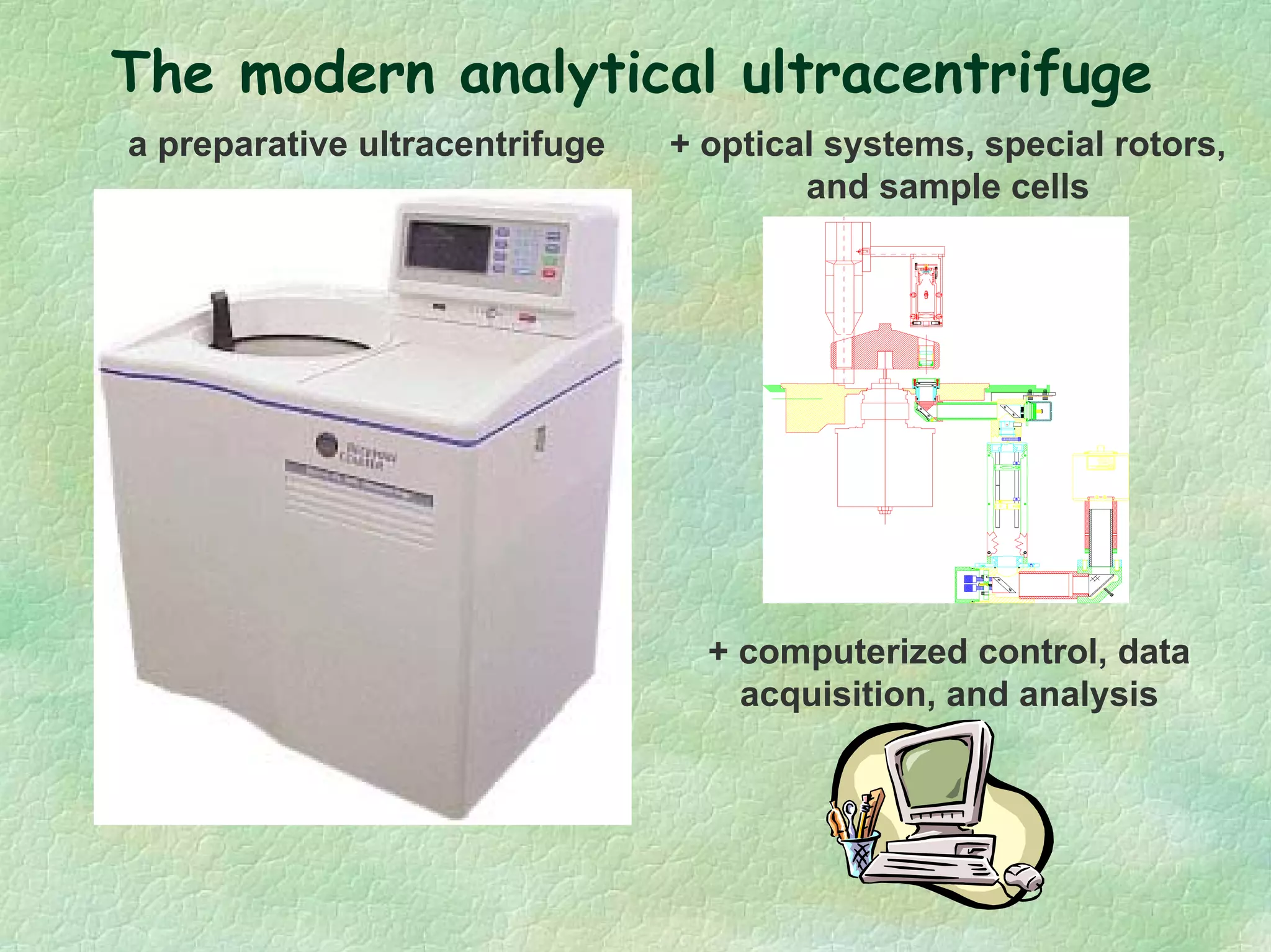
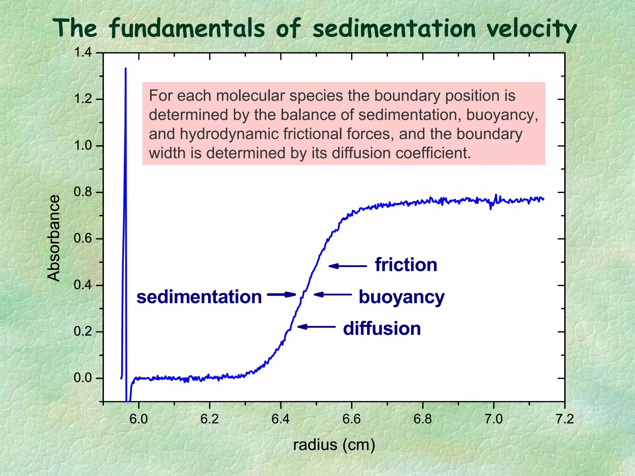
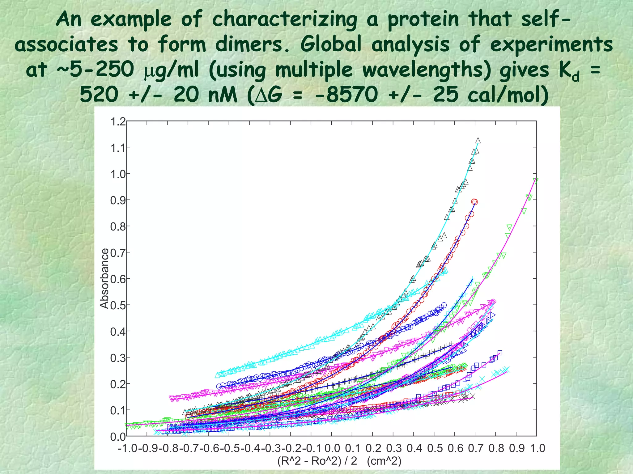
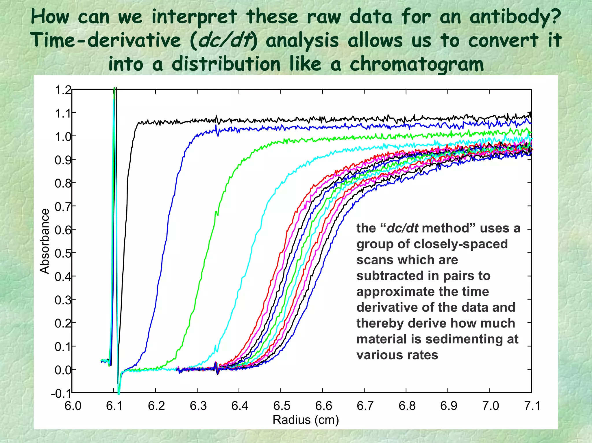
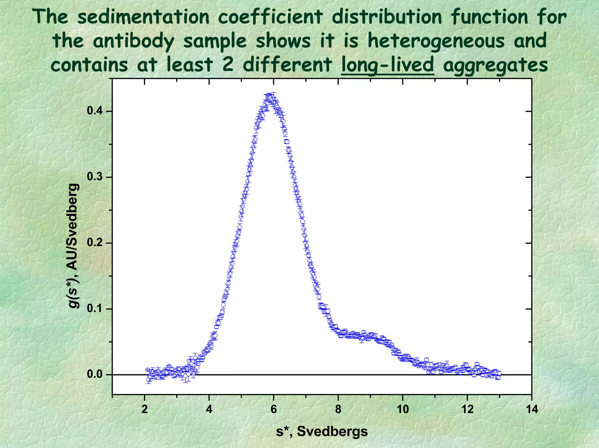
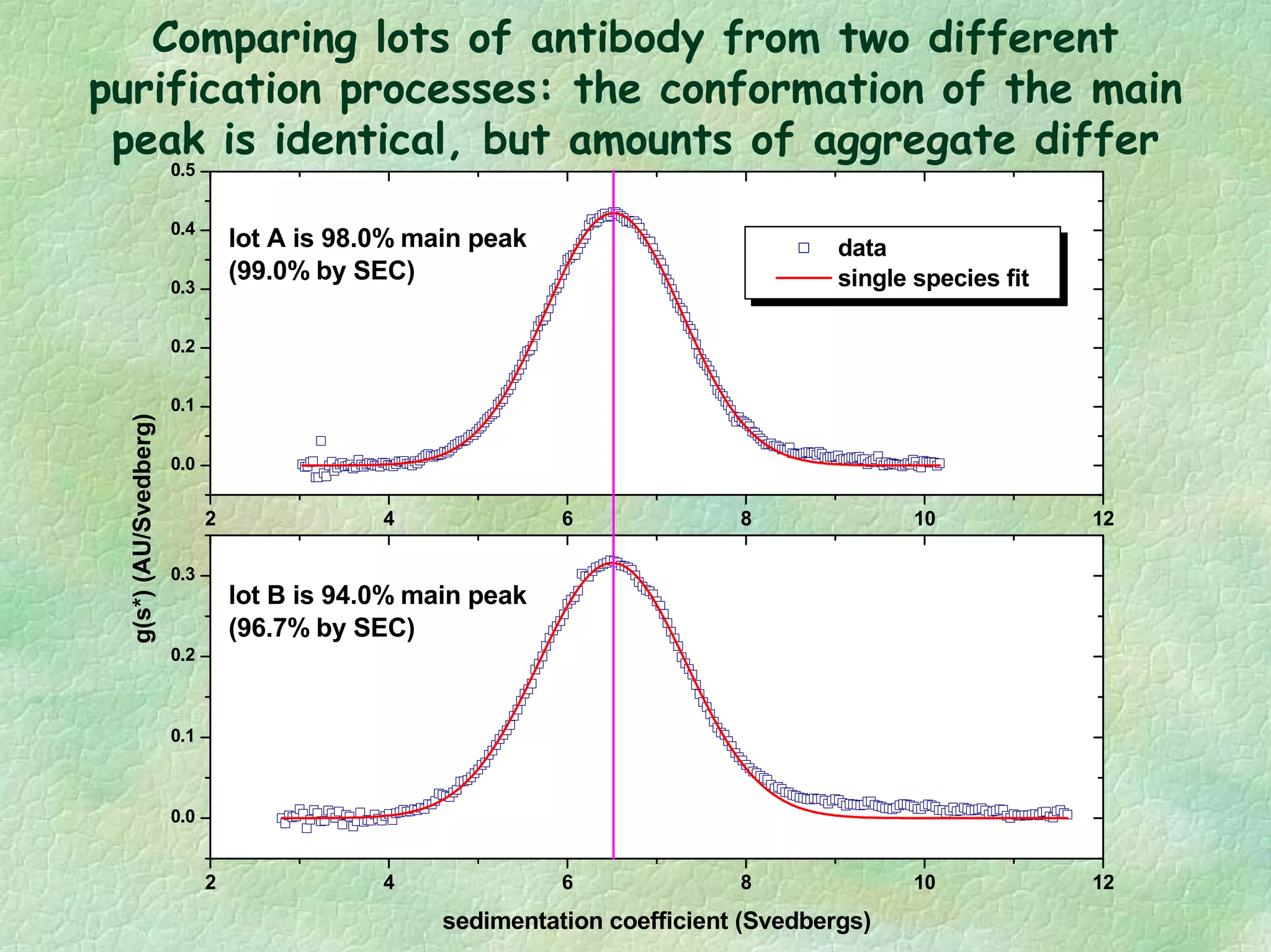
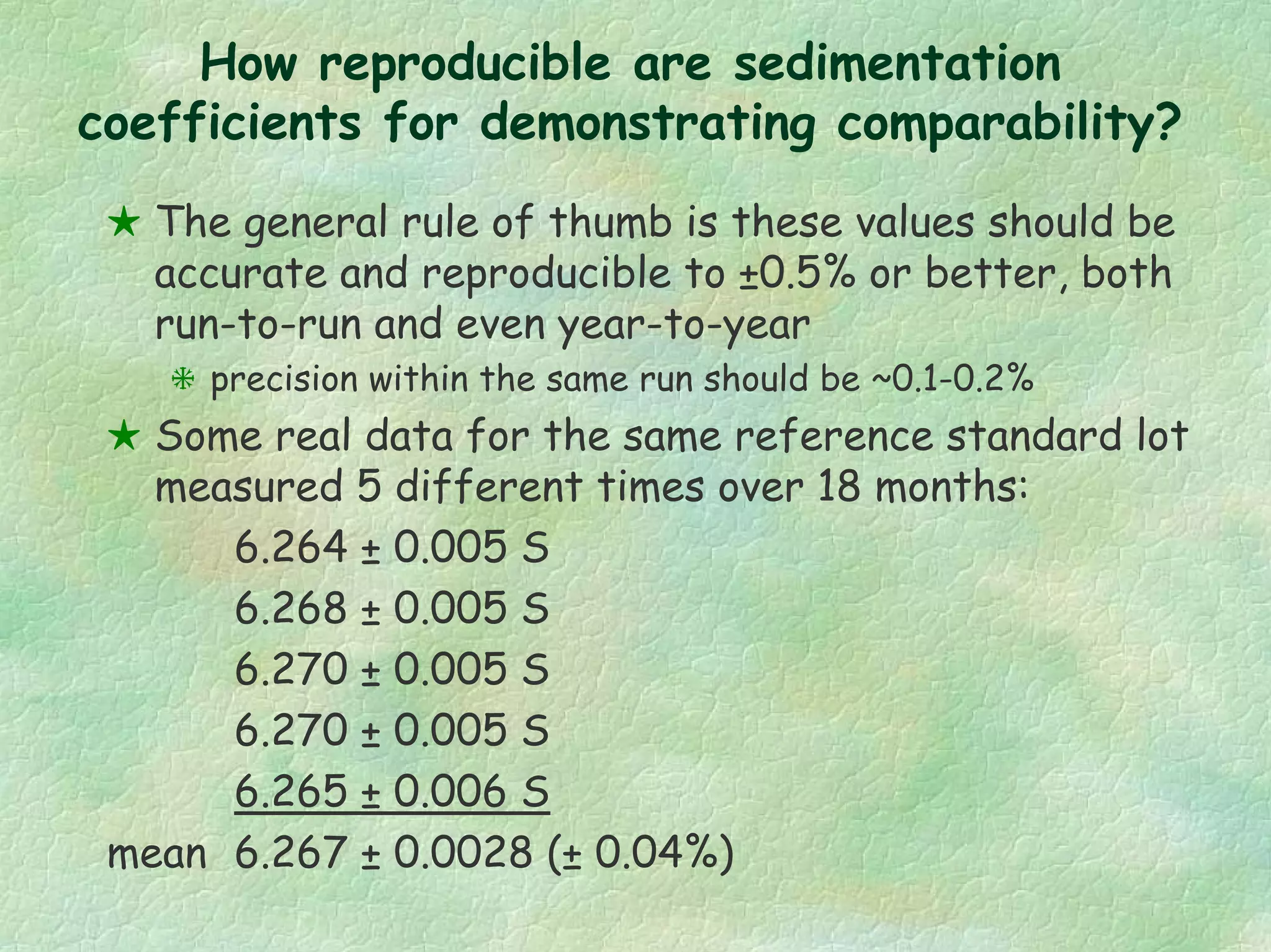
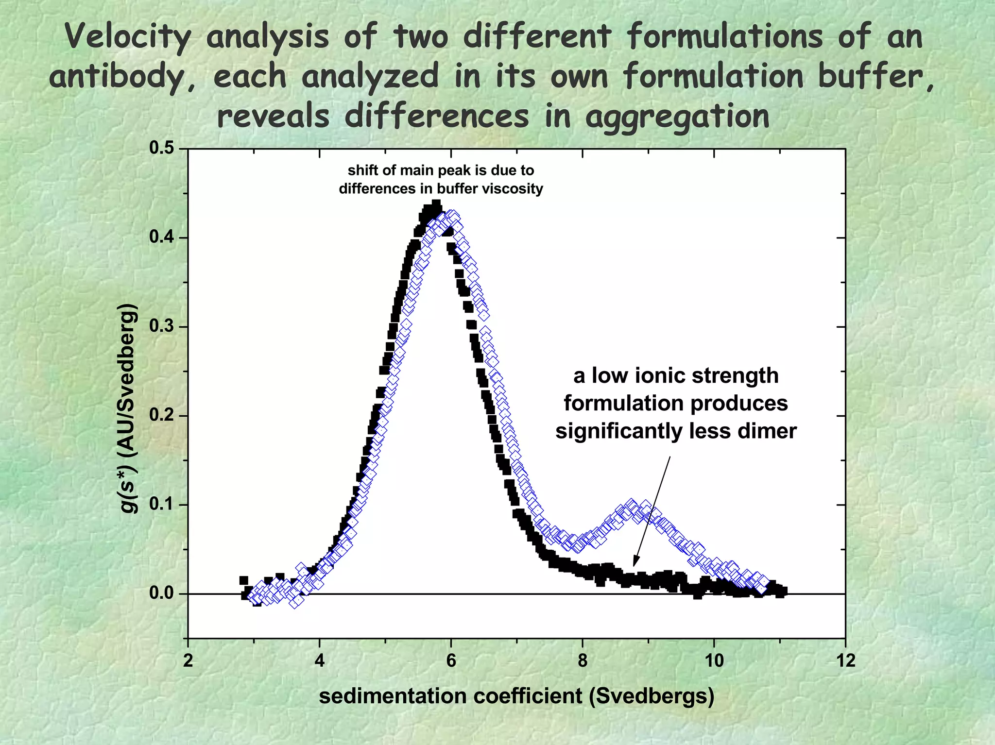
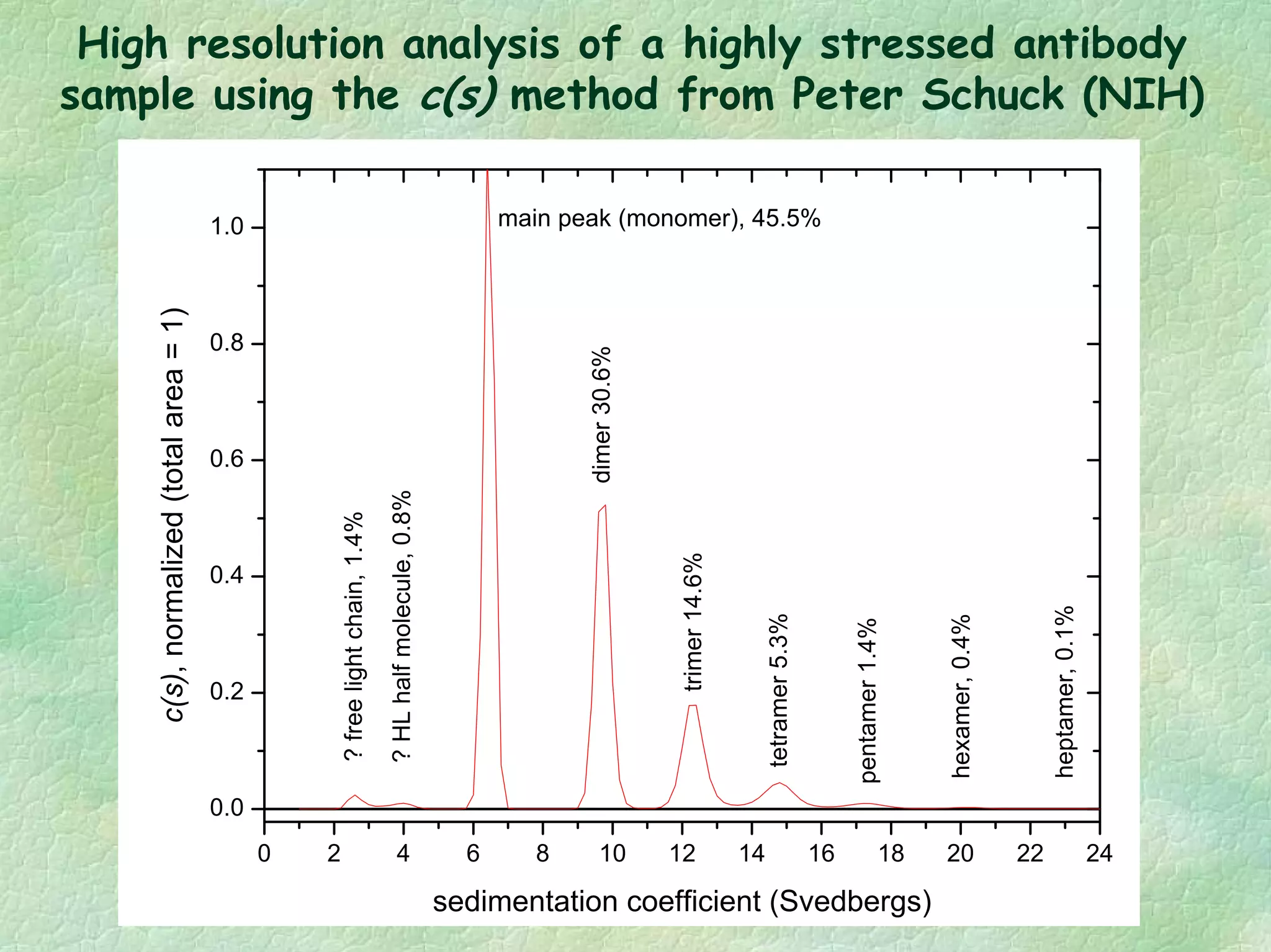
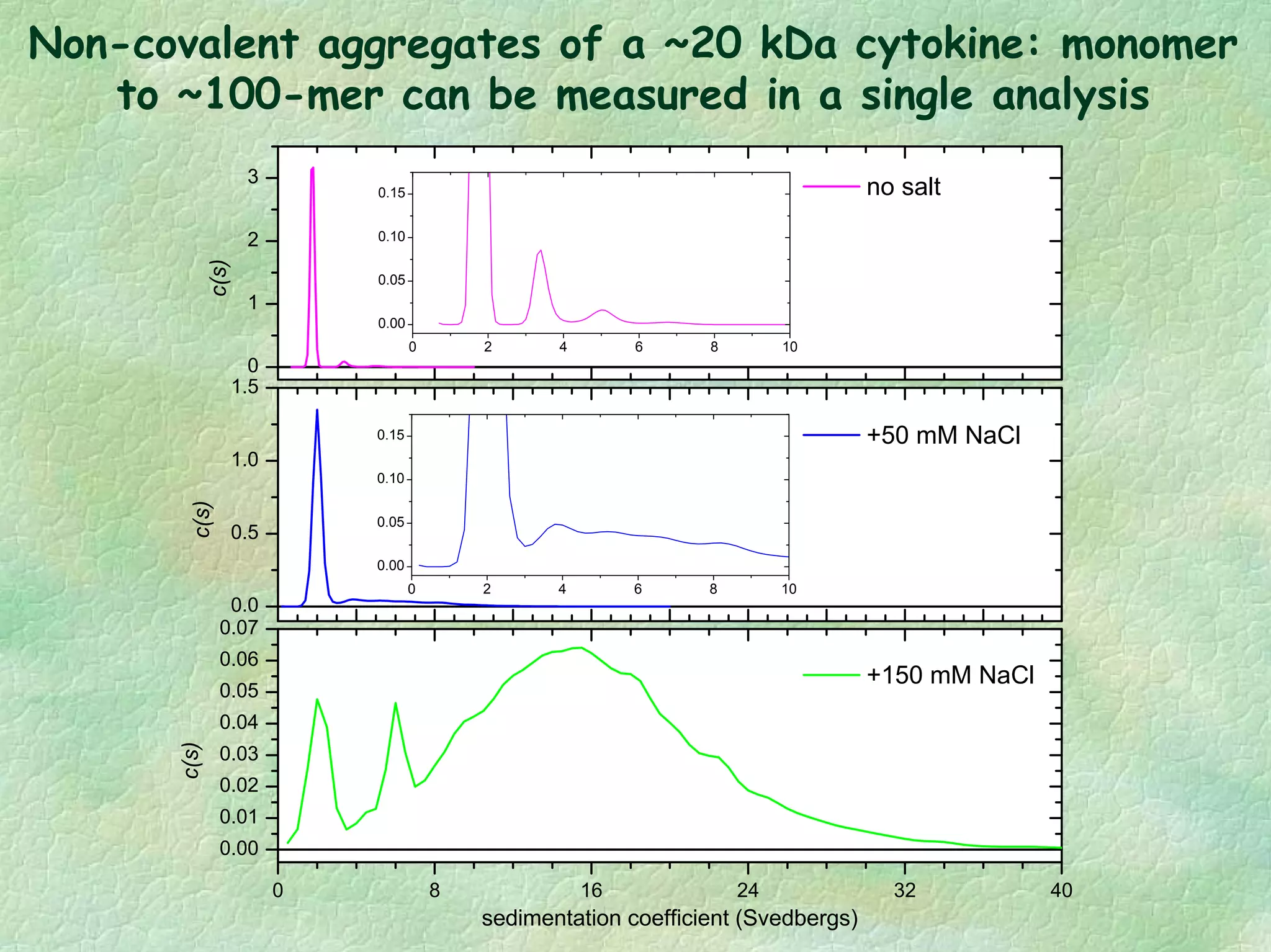
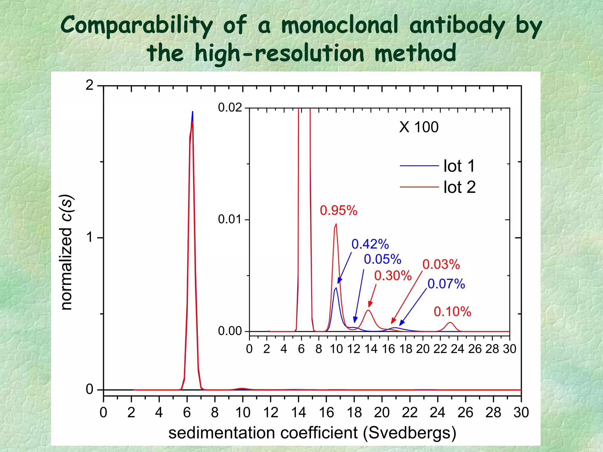
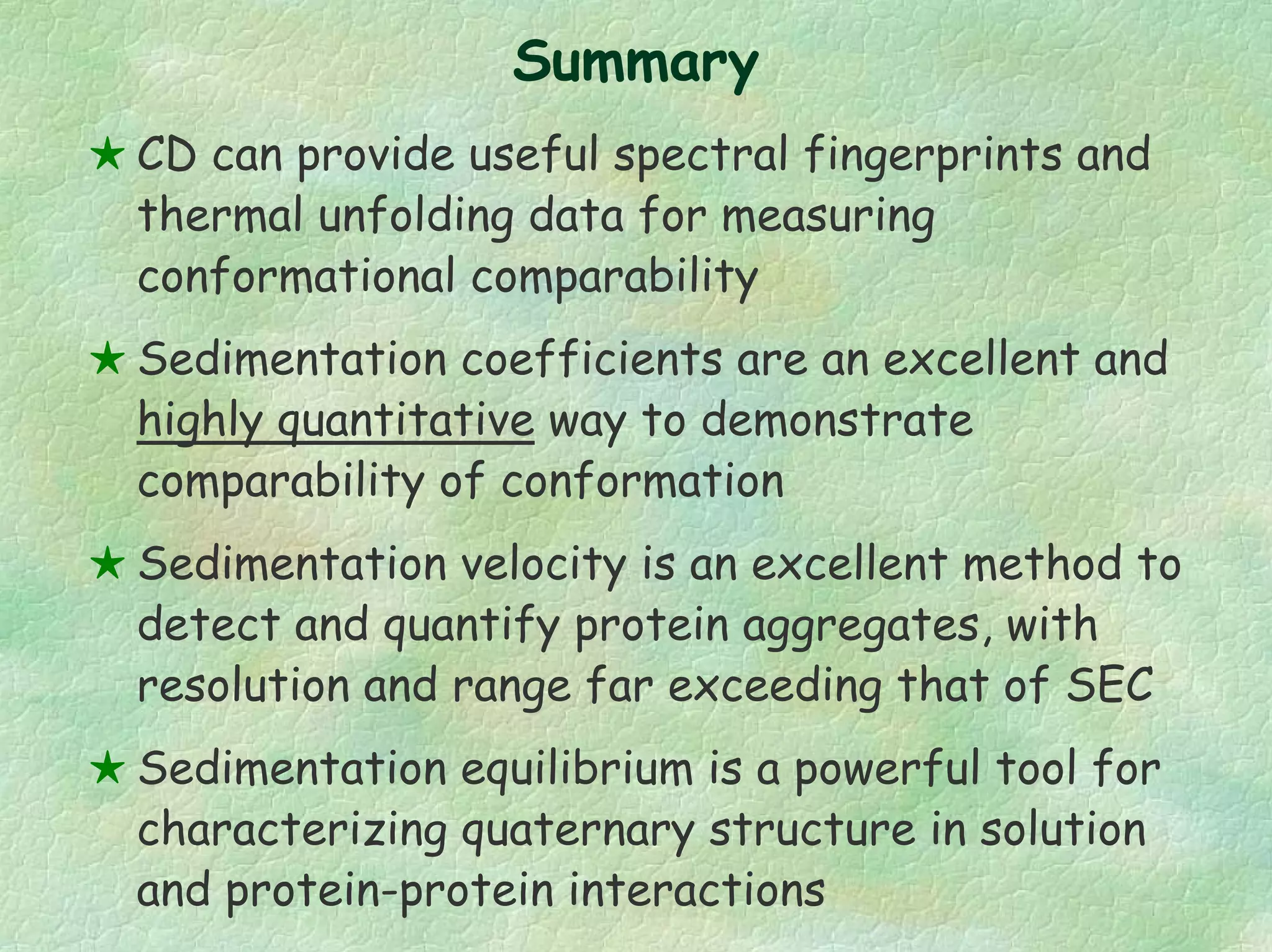
Measuring Comparability of
Conformation, Heterogeneity, and
Aggregation with Circular Dichroism
and Analytical Ultracentrifugation
John Philo
jphilo@ap-lab.com
© copyright 2003, Alliance Protein Laboratories Inc.
Outline
Circular dichroism---what does it do and
how can we apply it for comparability?
Introduction to analytical
ultracentrifugation: sedimentation velocity
and sedimentation equilibrium
Sedimentation equilibrium examples:
does my protein have the correct quaternary
structure?
Characterizing protein conformation and
aggregation by sedimentation velocity
Circular dichroism (CD) spectroscopy
measures the absorbance difference
between right-handed and left-
handed circularly polarized light
sensitive to chirality or asymmetry
around chromophores
Far-UV CD
‘far-UV’ protein
spectra (190-240
nm) are sensitive to
secondary structure
by spectral fitting
one can estimate
percentage α-helix,
β-sheet, etc.
our view: most useful
as comparative
spectral fingerprint 190 210 230 250
-40
-20
0
20
40
60
80
ellipticityperresiduex10
-3
(deg·cm/decimole)
alpha helix
beta sheet
random coil
wavelength (nm)
Differences in far-UV CD for natural vs.
recombinant forms of an enzyme (which
also have different enzymatic activity)
210 220 230 240 250 260
-12000
-10000
-8000
-6000
-4000
-2000
0
natural
recombinant
MolarEllipticity
W avelength (nm)
Near-UV CD
‘near-UV’ protein spectra (240-340 nm) are
sensitive to local tertiary structure around
aromatic residues and disulfide bonds
proteins lacking regular tertiary structure show
zero near-UV signal (e.g. “molten globules”)
signals can be either positive or negative
sometimes they nearly cancel
strictly a fingerprint---no direct structural
interpretation
our view:
under-utilized
usually more sensitive to subtle conformational
differences than far-UV
Differences in near-UV circular dichroism between
stable and unstable lots of a monoclonal antibody
240 250 260 270 280 290 300 310 320 330 340
-200
-150
-100
-50
0
50MolarEllipticity
Wavelength (nm)
lot 1
lot 2
Drawbacks to CD Spectral Analysis
1. difficult to quantitate similarity or
differences
what is “comparable” is often a judgment call
2. like all spectroscopy, if there is
heterogeneity all you see is an average
unlikely to detect minor components
3. certain buffer components absorb
strongly in the far-UV and can cause
interference
Measuring thermal stability (thermal
unfolding) by CD
Another conformational measure than can
be used for comparability
Very similar uses as DSC
can be done at much lower concentrations
can tell how the structure is changing, not just
that something is unfolding
Generally done by monitoring a single
wavelength in the far-UV vs. temperature
Quantitative analysis of thermal stability
from CD data
30 40 50 60 70
-80
-75
-70
-65
-60
-55
-50
-45
-40
melting
end (95%)
60.1 ± 0.5 °C
melting
onset (5%)
36.6 ± 0.4 °C
Tm
= 47.94 ± 0.14 °C,
∆H = 51.4 ± 3.2 kcal/mol
data
fit (2-state model)
molarellipticity@220nm
Temperature (°C)
Analytical
Ultracentrifugation
The modern analytical ultracentrifuge
a preparative ultracentrifuge
364371 DALSAINC.
CCDImageSensors
CL-E1-2048S-134L
S/NXXXXXX
MadeinCanada
+ optical systems, special rotors,
and sample cells
+ computerized control, data
acquisition, and analysis
6.0 6.2 6.4 6.6 6.8 7.0 7.2
0.0
0.2
0.4
0.6
0.8
1.0
1.2
1.4Absorbance
radius (cm)
meniscus
plateau
boundary
region of solute depletion
6.0 6.2 6.4 6.6 6.8 7.0 7.2
0.0
0.2
0.4
0.6
0.8
1.0
1.2
1.4Absorbance
radius (cm)
The sedimentation coefficient is
determined from the rate of boundary
motion. It depends on both molecular
weight and shape (conformation).
6.0 6.2 6.4 6.6 6.8 7.0 7.2
0.0
0.2
0.4
0.6
0.8
1.0
1.2
1.4Absorbance
radius (cm)
friction
diffusion
buoyancysedimentation
For each molecular species the boundary position is
determined by the balance of sedimentation, buoyancy,
and hydrodynamic frictional forces, and the boundary
width is determined by its diffusion coefficient.
The fundamentals of sedimentation velocity
6.30 6.35 6.40 6.45 6.50 6.55 6.60
0.0
0.2
0.4
0.6
0.8
1.0
cell base
Absorbance
radius (cm)
diffusion
buoyancysedimentation
meniscus
The fundamentals of sedimentation equilibrium
The concentration
distribution depends
only on molecular
weight, independent
of shape!
← smaller sample size to reduce time to reach equilibrium →
Both sedimentation methods are
“first principle” methods
based on fundamental physical laws
require no standard molecules for
calibration
calibration is based only on fundamental units
of distance, time, and temperature
Characterizing solution
mass by sedimentation
equilibrium
Size-exclusion chromatography of a TNF homolog
6 8 10 12 14 16 18 20
0.0
0.2
0.4
0.6
0.8
1.0
1.2
1.4
1.6
1.8
2.0absorbance(arb.units)
elution volume (ml)
ovalbumin
TNF homolog,
elutes exactly as
expected for a
17 kDa monomer
Linearized plot of equilibrium data for the TNF homolog
-0.6 -0.5 -0.4 -0.3 -0.2 -0.1 0.0 0.1 0.2 0.3 0.4 0.5 0.6
-1.9
-1.8
-1.7
-1.6
-1.5
-1.4
-1.3
-1.2
-1.1
-1.0
-0.9
-0.8
-0.7
-0.6
-0.5
-0.4
-0.3
-0.2
Ln(Absorbanceat230nm)
(r2 - ro
2 ) / 2
theoretical slope
for monomer
theoretical slope for trimer
An example of characterizing a protein that self-
associates to form dimers. Global analysis of experiments
at ~5-250 µg/ml (using multiple wavelengths) gives Kd =
520 +/- 20 nM (∆G = -8570 +/- 25 cal/mol)
-1.0-0.9-0.8-0.7-0.6-0.5-0.4-0.3-0.2-0.1 0.0 0.1 0.2 0.3 0.4 0.5 0.6 0.7 0.8 0.9 1.0
(R^2 - Ro^2) / 2 (cm^2)
0.0
0.1
0.2
0.3
0.4
0.5
0.6
0.7
0.8
0.9
1.0
1.1
1.2
Absorbance
Using sedimentation
velocity to characterize
protein conformation and
aggregation
How can we interpret these raw data for an antibody?
Time-derivative (dc/dt) analysis allows us to convert it
into a distribution like a chromatogram
6.0 6.1 6.2 6.3 6.4 6.5 6.6 6.7 6.8 6.9 7.0 7.1
Radius (cm)
-0.1
0.0
0.1
0.2
0.3
0.4
0.5
0.6
0.7
0.8
0.9
1.0
1.1
1.2
Absorbance
the “dc/dt method” uses a
group of closely-spaced
scans which are
subtracted in pairs to
approximate the time
derivative of the data and
thereby derive how much
material is sedimenting at
various rates
The sedimentation coefficient distribution function for
the antibody sample shows it is heterogeneous and
contains at least 2 different long-lived aggregates
2 4 6 8 10 12 14
0.0
0.1
0.2
0.3
0.4
g(s*),AU/Svedberg
s*, Svedbergs
Comparing lots of antibody from two different
purification processes: the conformation of the main
peak is identical, but amounts of aggregate differ
2 4 6 8 10 12
0.0
0.1
0.2
0.3
lot B is 94.0% main peak
(96.7% by SEC)
g(s*)(AU/Svedberg)
sedimentation coefficient (Svedbergs)
2 4 6 8 10 12
0.0
0.1
0.2
0.3
0.4
0.5
data
single species fit
lot A is 98.0% main peak
(99.0% by SEC)
How reproducible are sedimentation
coefficients for demonstrating comparability?
The general rule of thumb is these values should be
accurate and reproducible to ±0.5% or better, both
run-to-run and even year-to-year
precision within the same run should be ~0.1-0.2%
Some real data for the same reference standard lot
measured 5 different times over 18 months:
6.264 ± 0.005 S
6.268 ± 0.005 S
6.270 ± 0.005 S
6.270 ± 0.005 S
6.265 ± 0.006 S
mean 6.267 ± 0.0028 (± 0.04%)
Velocity analysis of two different formulations of an
antibody, each analyzed in its own formulation buffer,
reveals differences in aggregation
2 4 6 8 10 12
0.0
0.1
0.2
0.3
0.4
0.5
a low ionic strength
formulation produces
significantly less dimer
shift of main peak is due to
differences in buffer viscosity
g(s*)(AU/Svedberg)
sedimentation coefficient (Svedbergs)
High resolution analysis of a highly stressed antibody
sample using the c(s) method from Peter Schuck (NIH)
0 2 4 6 8 10 12 14 16 18 20 22 24
0.0
0.2
0.4
0.6
0.8
1.0
heptamer,0.1%
hexamer,0.4%
pentamer1.4%
tetramer5.3%
trimer14.6%
dimer30.6%
main peak (monomer), 45.5%
?HLhalfmolecule,0.8%
?freelightchain,1.4%
c(s),normalized(totalarea=1)
sedimentation coefficient (Svedbergs)
0
1
2
3
0.0
0.5
1.0
1.5
0 8 16 24 32 40
0.00
0.01
0.02
0.03
0.04
0.05
0.06
0.07
no salt
c(s)
+50 mM NaCl
c(s)
+150 mM NaCl
c(s)
sedimentation coefficient (Svedbergs)
0 2 4 6 8 10
0.00
0.05
0.10
0.15
20X expanded
0 2 4 6 8 10
0.00
0.05
0.10
0.15
20X expanded
Non-covalent aggregates of a ~20 kDa cytokine: monomer
to ~100-mer can be measured in a single analysis
Comparability of a monoclonal antibody by
the high-resolution method
0 2 4 6 8 10 12 14 16 18 20 22 24 26 28 30
0
1
2
0 2 4 6 8 10 12 14 16 18 20 22 24 26 28 30
0.00
0.01
0.02
normalizedc(s)
sedimentation coefficient (Svedbergs)
0.42%
0.10%
0.03%
0.30%
lot 1
lot 2
X 100
0.95%
0.05%
0.07%
“Aggregates” vs. self-associated oligomers
We must be careful to distinguish between
rapidly-reversible, self-associated
oligomers and irreversible (or at least long-
lived) oligomers (“aggregates”)
distinction more important now that we are
seeing so many high concentration formulations
Oligomers which are reversible, but which
dissociate only over hours-days, are much
more common than most people realize
Our View: only the long-lived (hours or
more) aggregates are likely to have an
impact on immunogenicity, PK, or efficacy
oligomers which rapidly dissociate upon dilution
in vivo are unlikely to impact safety or efficacy
These same velocity methods can be
applied to other biopharmaceuticals besides
pure recombinant proteins
1. protein mixtures such as blood products
2. nucleic acids
naked vaccines
gene therapy
ribozymes
3. whole virus
vaccines
gene therapy vectors
4. drug-polypeptide conjugates
toxin:antibody conjugates
small-molecule:poly-amino acid conjugates
Summary
CD can provide useful spectral fingerprints and
thermal unfolding data for measuring
conformational comparability
Sedimentation coefficients are an excellent and
highly quantitative way to demonstrate
comparability of conformation
Sedimentation velocity is an excellent method to
detect and quantify protein aggregates, with
resolution and range far exceeding that of SEC
Sedimentation equilibrium is a powerful tool for
characterizing quaternary structure in solution
and protein-protein interactions

Measuring Comparability of Conformation, Heterogeneity and Aggregation with Circular Dichroism and Analytical Ultracentrifugation

  • 1.
    Measuring Comparability of Conformation,Heterogeneity, and Aggregation with Circular Dichroism and Analytical Ultracentrifugation John Philo jphilo@ap-lab.com © copyright 2003, Alliance Protein Laboratories Inc.
  • 2.
    Outline Circular dichroism---what doesit do and how can we apply it for comparability? Introduction to analytical ultracentrifugation: sedimentation velocity and sedimentation equilibrium Sedimentation equilibrium examples: does my protein have the correct quaternary structure? Characterizing protein conformation and aggregation by sedimentation velocity
  • 3.
    Circular dichroism (CD)spectroscopy measures the absorbance difference between right-handed and left- handed circularly polarized light sensitive to chirality or asymmetry around chromophores
  • 4.
    Far-UV CD ‘far-UV’ protein spectra(190-240 nm) are sensitive to secondary structure by spectral fitting one can estimate percentage α-helix, β-sheet, etc. our view: most useful as comparative spectral fingerprint 190 210 230 250 -40 -20 0 20 40 60 80 ellipticityperresiduex10 -3 (deg·cm/decimole) alpha helix beta sheet random coil wavelength (nm)
  • 5.
    Differences in far-UVCD for natural vs. recombinant forms of an enzyme (which also have different enzymatic activity) 210 220 230 240 250 260 -12000 -10000 -8000 -6000 -4000 -2000 0 natural recombinant MolarEllipticity W avelength (nm)
  • 6.
    Near-UV CD ‘near-UV’ proteinspectra (240-340 nm) are sensitive to local tertiary structure around aromatic residues and disulfide bonds proteins lacking regular tertiary structure show zero near-UV signal (e.g. “molten globules”) signals can be either positive or negative sometimes they nearly cancel strictly a fingerprint---no direct structural interpretation our view: under-utilized usually more sensitive to subtle conformational differences than far-UV
  • 7.
    Differences in near-UVcircular dichroism between stable and unstable lots of a monoclonal antibody 240 250 260 270 280 290 300 310 320 330 340 -200 -150 -100 -50 0 50MolarEllipticity Wavelength (nm) lot 1 lot 2
  • 8.
    Drawbacks to CDSpectral Analysis 1. difficult to quantitate similarity or differences what is “comparable” is often a judgment call 2. like all spectroscopy, if there is heterogeneity all you see is an average unlikely to detect minor components 3. certain buffer components absorb strongly in the far-UV and can cause interference
  • 9.
    Measuring thermal stability(thermal unfolding) by CD Another conformational measure than can be used for comparability Very similar uses as DSC can be done at much lower concentrations can tell how the structure is changing, not just that something is unfolding Generally done by monitoring a single wavelength in the far-UV vs. temperature
  • 10.
    Quantitative analysis ofthermal stability from CD data 30 40 50 60 70 -80 -75 -70 -65 -60 -55 -50 -45 -40 melting end (95%) 60.1 ± 0.5 °C melting onset (5%) 36.6 ± 0.4 °C Tm = 47.94 ± 0.14 °C, ∆H = 51.4 ± 3.2 kcal/mol data fit (2-state model) molarellipticity@220nm Temperature (°C)
  • 11.
  • 12.
    The modern analyticalultracentrifuge a preparative ultracentrifuge 364371 DALSAINC. CCDImageSensors CL-E1-2048S-134L S/NXXXXXX MadeinCanada + optical systems, special rotors, and sample cells + computerized control, data acquisition, and analysis
  • 13.
    6.0 6.2 6.46.6 6.8 7.0 7.2 0.0 0.2 0.4 0.6 0.8 1.0 1.2 1.4Absorbance radius (cm) meniscus plateau boundary region of solute depletion 6.0 6.2 6.4 6.6 6.8 7.0 7.2 0.0 0.2 0.4 0.6 0.8 1.0 1.2 1.4Absorbance radius (cm) The sedimentation coefficient is determined from the rate of boundary motion. It depends on both molecular weight and shape (conformation). 6.0 6.2 6.4 6.6 6.8 7.0 7.2 0.0 0.2 0.4 0.6 0.8 1.0 1.2 1.4Absorbance radius (cm) friction diffusion buoyancysedimentation For each molecular species the boundary position is determined by the balance of sedimentation, buoyancy, and hydrodynamic frictional forces, and the boundary width is determined by its diffusion coefficient. The fundamentals of sedimentation velocity
  • 14.
    6.30 6.35 6.406.45 6.50 6.55 6.60 0.0 0.2 0.4 0.6 0.8 1.0 cell base Absorbance radius (cm) diffusion buoyancysedimentation meniscus The fundamentals of sedimentation equilibrium The concentration distribution depends only on molecular weight, independent of shape! ← smaller sample size to reduce time to reach equilibrium →
  • 15.
    Both sedimentation methodsare “first principle” methods based on fundamental physical laws require no standard molecules for calibration calibration is based only on fundamental units of distance, time, and temperature
  • 16.
    Characterizing solution mass bysedimentation equilibrium
  • 17.
    Size-exclusion chromatography ofa TNF homolog 6 8 10 12 14 16 18 20 0.0 0.2 0.4 0.6 0.8 1.0 1.2 1.4 1.6 1.8 2.0absorbance(arb.units) elution volume (ml) ovalbumin TNF homolog, elutes exactly as expected for a 17 kDa monomer
  • 18.
    Linearized plot ofequilibrium data for the TNF homolog -0.6 -0.5 -0.4 -0.3 -0.2 -0.1 0.0 0.1 0.2 0.3 0.4 0.5 0.6 -1.9 -1.8 -1.7 -1.6 -1.5 -1.4 -1.3 -1.2 -1.1 -1.0 -0.9 -0.8 -0.7 -0.6 -0.5 -0.4 -0.3 -0.2 Ln(Absorbanceat230nm) (r2 - ro 2 ) / 2 theoretical slope for monomer theoretical slope for trimer
  • 19.
    An example ofcharacterizing a protein that self- associates to form dimers. Global analysis of experiments at ~5-250 µg/ml (using multiple wavelengths) gives Kd = 520 +/- 20 nM (∆G = -8570 +/- 25 cal/mol) -1.0-0.9-0.8-0.7-0.6-0.5-0.4-0.3-0.2-0.1 0.0 0.1 0.2 0.3 0.4 0.5 0.6 0.7 0.8 0.9 1.0 (R^2 - Ro^2) / 2 (cm^2) 0.0 0.1 0.2 0.3 0.4 0.5 0.6 0.7 0.8 0.9 1.0 1.1 1.2 Absorbance
  • 20.
    Using sedimentation velocity tocharacterize protein conformation and aggregation
  • 21.
    How can weinterpret these raw data for an antibody? Time-derivative (dc/dt) analysis allows us to convert it into a distribution like a chromatogram 6.0 6.1 6.2 6.3 6.4 6.5 6.6 6.7 6.8 6.9 7.0 7.1 Radius (cm) -0.1 0.0 0.1 0.2 0.3 0.4 0.5 0.6 0.7 0.8 0.9 1.0 1.1 1.2 Absorbance the “dc/dt method” uses a group of closely-spaced scans which are subtracted in pairs to approximate the time derivative of the data and thereby derive how much material is sedimenting at various rates
  • 22.
    The sedimentation coefficientdistribution function for the antibody sample shows it is heterogeneous and contains at least 2 different long-lived aggregates 2 4 6 8 10 12 14 0.0 0.1 0.2 0.3 0.4 g(s*),AU/Svedberg s*, Svedbergs
  • 23.
    Comparing lots ofantibody from two different purification processes: the conformation of the main peak is identical, but amounts of aggregate differ 2 4 6 8 10 12 0.0 0.1 0.2 0.3 lot B is 94.0% main peak (96.7% by SEC) g(s*)(AU/Svedberg) sedimentation coefficient (Svedbergs) 2 4 6 8 10 12 0.0 0.1 0.2 0.3 0.4 0.5 data single species fit lot A is 98.0% main peak (99.0% by SEC)
  • 24.
    How reproducible aresedimentation coefficients for demonstrating comparability? The general rule of thumb is these values should be accurate and reproducible to ±0.5% or better, both run-to-run and even year-to-year precision within the same run should be ~0.1-0.2% Some real data for the same reference standard lot measured 5 different times over 18 months: 6.264 ± 0.005 S 6.268 ± 0.005 S 6.270 ± 0.005 S 6.270 ± 0.005 S 6.265 ± 0.006 S mean 6.267 ± 0.0028 (± 0.04%)
  • 25.
    Velocity analysis oftwo different formulations of an antibody, each analyzed in its own formulation buffer, reveals differences in aggregation 2 4 6 8 10 12 0.0 0.1 0.2 0.3 0.4 0.5 a low ionic strength formulation produces significantly less dimer shift of main peak is due to differences in buffer viscosity g(s*)(AU/Svedberg) sedimentation coefficient (Svedbergs)
  • 26.
    High resolution analysisof a highly stressed antibody sample using the c(s) method from Peter Schuck (NIH) 0 2 4 6 8 10 12 14 16 18 20 22 24 0.0 0.2 0.4 0.6 0.8 1.0 heptamer,0.1% hexamer,0.4% pentamer1.4% tetramer5.3% trimer14.6% dimer30.6% main peak (monomer), 45.5% ?HLhalfmolecule,0.8% ?freelightchain,1.4% c(s),normalized(totalarea=1) sedimentation coefficient (Svedbergs)
  • 27.
    0 1 2 3 0.0 0.5 1.0 1.5 0 8 1624 32 40 0.00 0.01 0.02 0.03 0.04 0.05 0.06 0.07 no salt c(s) +50 mM NaCl c(s) +150 mM NaCl c(s) sedimentation coefficient (Svedbergs) 0 2 4 6 8 10 0.00 0.05 0.10 0.15 20X expanded 0 2 4 6 8 10 0.00 0.05 0.10 0.15 20X expanded Non-covalent aggregates of a ~20 kDa cytokine: monomer to ~100-mer can be measured in a single analysis
  • 28.
    Comparability of amonoclonal antibody by the high-resolution method 0 2 4 6 8 10 12 14 16 18 20 22 24 26 28 30 0 1 2 0 2 4 6 8 10 12 14 16 18 20 22 24 26 28 30 0.00 0.01 0.02 normalizedc(s) sedimentation coefficient (Svedbergs) 0.42% 0.10% 0.03% 0.30% lot 1 lot 2 X 100 0.95% 0.05% 0.07%
  • 29.
    “Aggregates” vs. self-associatedoligomers We must be careful to distinguish between rapidly-reversible, self-associated oligomers and irreversible (or at least long- lived) oligomers (“aggregates”) distinction more important now that we are seeing so many high concentration formulations Oligomers which are reversible, but which dissociate only over hours-days, are much more common than most people realize Our View: only the long-lived (hours or more) aggregates are likely to have an impact on immunogenicity, PK, or efficacy oligomers which rapidly dissociate upon dilution in vivo are unlikely to impact safety or efficacy
  • 30.
    These same velocitymethods can be applied to other biopharmaceuticals besides pure recombinant proteins 1. protein mixtures such as blood products 2. nucleic acids naked vaccines gene therapy ribozymes 3. whole virus vaccines gene therapy vectors 4. drug-polypeptide conjugates toxin:antibody conjugates small-molecule:poly-amino acid conjugates
  • 31.
    Summary CD can provideuseful spectral fingerprints and thermal unfolding data for measuring conformational comparability Sedimentation coefficients are an excellent and highly quantitative way to demonstrate comparability of conformation Sedimentation velocity is an excellent method to detect and quantify protein aggregates, with resolution and range far exceeding that of SEC Sedimentation equilibrium is a powerful tool for characterizing quaternary structure in solution and protein-protein interactions