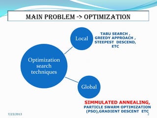
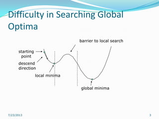
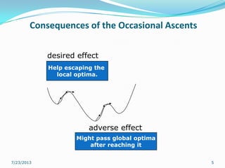
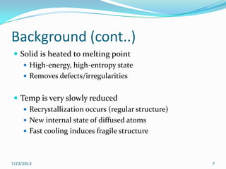
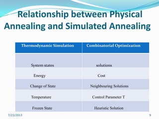
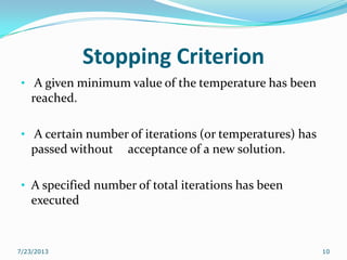
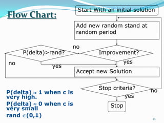
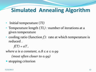
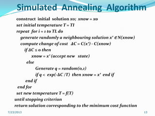
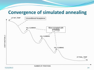
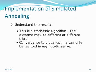
The document discusses simulated annealing (SA), a global optimization technique inspired by the physical process of annealing in solids, characterized by its ability to escape local optima. It explains the mechanics of SA, its stopping criteria, advantages, and applications in various fields such as circuit partitioning and image processing. Additionally, it compares SA's effectiveness against greedy algorithms, particularly in problems with numerous local optima.

1. 7/23/2013 1

2. MAIN PROBLEM -> OPTIMIZATION
Local
Global
Optimization
search
techniques
7/23/2013 2
TABU SEARCH ,
GREEDY APPROACH ,
STEEPEST DESCEND,
ETC
SIMMULATED ANNEALING,
PARTICLE SWARM OPTIMIZATION
(PSO),GRADIENT DESCENT ETC

3. Difficulty in Searching Global
Optima
7/23/2013 3
starting
point
descend
direction
local minima
global minima
barrier to local search

4. Simulated Annealing(SA)
• SA is a global optimization technique.
• SA distinguishes between different local optima.
 SA is a memory less algorithm, the algorithm does not use
any information gathered during the search
 SA is motivated by an analogy to annealing in solids.
 Simulated Annealing – an iterative improvement
algorithm.
7/23/2013 4

5. Consequences of the Occasional Ascents
7/23/2013 5
Help escaping the
local optima.
desired effect
Might pass global optima
after reaching it
adverse effect

6. Background: Annealing
 Simulated annealing is so named because of its analogy to the process
of physical annealing with solids,.
 A crystalline solid is heated and then allowed to cool very slowly
 until it achieves its most regular possible crystal lattice configuration
(i.e., its minimum lattice energy state), and thus is free of crystal
defects.
 If the cooling schedule is sufficiently slow, the final configuration
results in a solid with such superior structural integrity.
 Simulated annealing establishes the connection between this type of
thermodynamic behaviour and the search for global minima for a
discrete optimization problem.
7/23/2013 6

7. Background (cont..)
 Solid is heated to melting point
 High-energy, high-entropy state
 Removes defects/irregularities
 Temp is very slowly reduced
 Recrystallization occurs (regular structure)
 New internal state of diffused atoms
 Fast cooling induces fragile structure
7/23/2013 7

8. Control of Annealing Process
7/23/2013 8
Acceptance of a search step (Metropolis
Criterion):
Assume the performance change in the
search direction is .
Accept a ascending step only if it pass a
random test,
Always accept a descending step, i.e. 0
1,0exp randomT

9. Relationship between Physical
Annealing and Simulated Annealing
Thermodynamic Simulation Combinatorial Optimization
System states solutions
Energy Cost
Change of State Neighbouring Solutions
Temperature Control Parameter T
Frozen State Heuristic Solution
7/23/2013 9

10. Stopping Criterion
• A given minimum value of the temperature has been
reached.
• A certain number of iterations (or temperatures) has
passed without acceptance of a new solution.
• A specified number of total iterations has been
executed
7/23/2013 10

11. 11
Flow Chart:
Start With an initial solution
Add new random stand at
random period
Improvement?
Accept new Solution
Stop criteria?
Stop
P(delta)>rand?
yes
yes
yes
no
no
noP(delta) 1 when c is
very high.
P(delta) 0 when c is
very small
rand (0,1)

12. Simulated Annealing Algorithm
• Initial temperature (TI)
• Temperature length (TL) : number of iterations at a
given temperature
• cooling ratio (function f): rate at which temperature is
reduced .
f(T) = aT ,
where a is a constant, 0.8 ≤ a ≤ 0.99
(most often closer to 0.99)
 stopping criterion
7/23/2013 12

13. Simulated Annealing Algorithm
construct initial solution x0; xnow = x0
set initial temperature T = TI
repeat for i = 1 to TL do
generate randomly a neighbouring solution x′ ∈ N(xnow)
compute change of cost ΔC = C(x′) - C(xnow)
if ΔC ≤ 0 then
xnow = x′ (accept new state)
else
Generate q = random(0,1)
if q < exp(-ΔC /T) then xnow = x′ end if
end if
end for
set new temperature T = f(T)
until stopping criterion
return solution corresponding to the minimum cost function
7/23/2013 13

14. Convergence of simulated annealing
HILL CLIMBING
HILL CLIMBING
HILL CLIMBING
COSTFUNCTION,C
NUMBER OF ITERATIONS
AT INIT_TEMP
AT FINAL_TEMP
Move accepted with
probability
= e-(^C/temp)
Unconditional Acceptance
7/23/2013 14

15. Implementation of Simulated
Annealing
7/23/2013 15
 Understand the result:
• This is a stochastic algorithm. The
outcome may be different at different
trials.
• Convergence to global optima can only
be realized in asymptotic sense.

16. Qualitative Analysis
 Randomized local search.
 Is simulated annealing greedy?
 Controlled greed.
 Is a greedy algorithm better? Where is the
difference?
 Explain with - The ball-on-terrain example.
7/23/2013 16

17. Ball on terrain example – Simulated
Annealing vs Greedy Algorithms
• The ball is initially placed at a random
position on the terrain. From the current
position, the ball should be fired such that
it can only move one step left or right.
What algorithm should we follow for the
ball to finally settle at the lowest point on
the terrain?
7/23/2013 17

18. Ball on terrain example – SA vs. Greedy
Algorithms
Greedy Algorithm
gets stuck here!
Locally Optimum
Solution.
Simulated Annealing explores
more. Chooses this move with a
small probability (Hill Climbing)
Upon a large no. of iterations,
SA converges to this solution.
Initial position
of the ball
7/23/2013 18

19. Jigsaw puzzles – Intuitive usage of
Simulated Annealing
• Given a jigsaw puzzle such
that one has to obtain the
final shape using all pieces
together.
• Starting with a random
configuration, the human
brain unconditionally
chooses certain moves that
tend to the solution.
• However, certain moves that
may or may not lead to the
solution are accepted or
rejected with a certain small
probability.
• The final shape is obtained
as a result of a large
number of iterations.
7/23/2013 19

20. Applications
 Circuit partitioning and placement.
 Hardware/Software Partitioning
 Graph partitioning
 VLSI: Placement, routing.
 Image processing
 Strategy scheduling for capital products with complex
product structure.
 Umpire scheduling in US Open Tennis tournament!
 Event-based learning situations.
 etc
7/23/2013 20

21. 7/23/2013 21
Advantages:
• can deal with arbitrary systems and cost functions
• statistically guarantees finding an optimal solution
• is relatively easy to code, even for complex
problems.
• generally gives a ``good'' solution
This makes annealing an attractive option for
optimization problems where heuristic (specialized
or problem specific) methods are not available.

22. 7/23/2013 22
•Repeatedly annealing with a 1/log k schedule is very slow,
especially if the cost function is expensive to compute.
•For problems where the energy landscape is smooth, or there are
few local minima, SA is overkill - simpler, faster methods (e.g.,
gradient descent) will work better. But generally don't know what
the energy landscape is for a particular problem.
•Heuristic methods, which are problem-specific or take advantage of
extra information about the system, will often be better than general
methods, although SA is often comparable to heuristics.
•The method cannot tell whether it has found an optimal solution.
Some other complimentary method (e.g. branch and bound) is
required to do this.

23. Conclusions
 Simulated Annealing algorithms are usually better
than greedy algorithms, when it comes to
problems that have numerous locally optimum
solutions.
 Simulated Annealing is not the best solution to
circuit partitioning or placement. Network flow
approach to solving these problems functions
much faster.
 Simulated Annealing guarantees a convergence
upon running sufficiently large number of
iterations.
7/23/2013 23

24. Reference:
7/23/2013 24
• P.J.M. van Laarhoven, E.H.L. Aarts, Simulated Annealing:
Theory and Applications, Kluwer Academic Publisher,
1987.
• A. A. Zhigljavsky, Theory of Global Random Search,
Kluwer Academic Publishers, 1991.