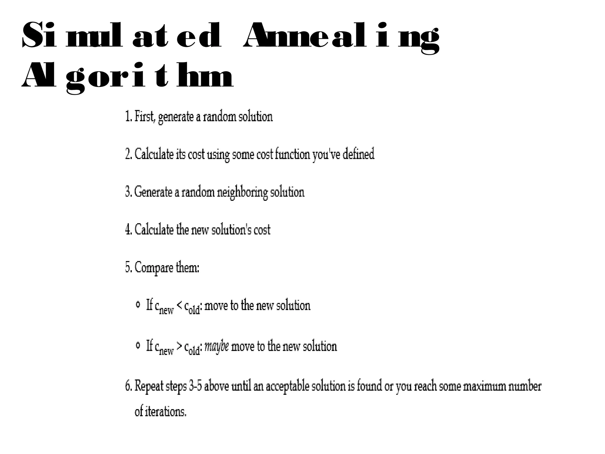
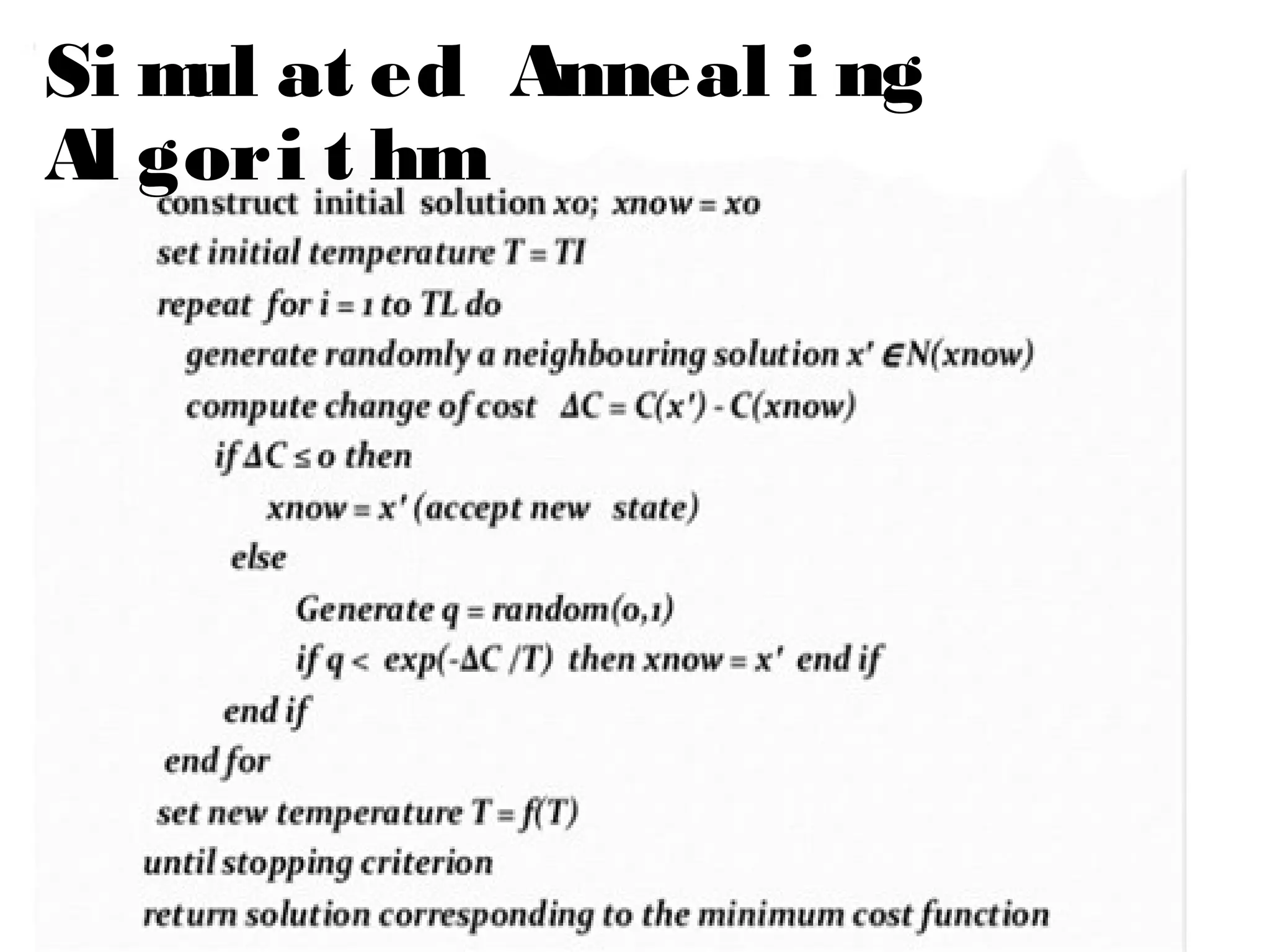
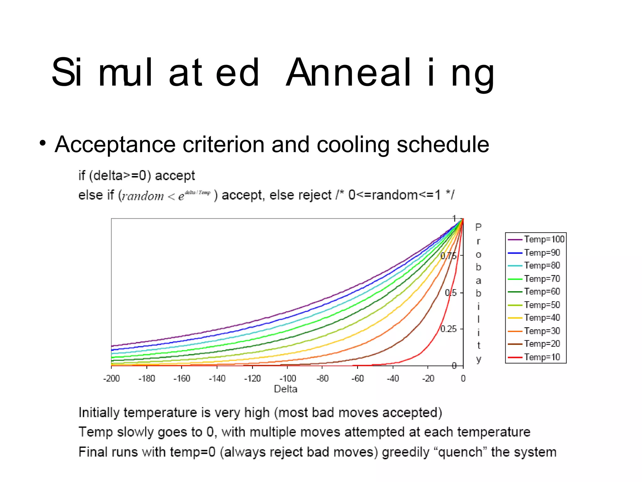
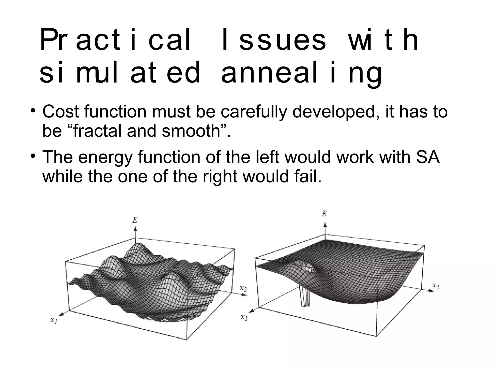
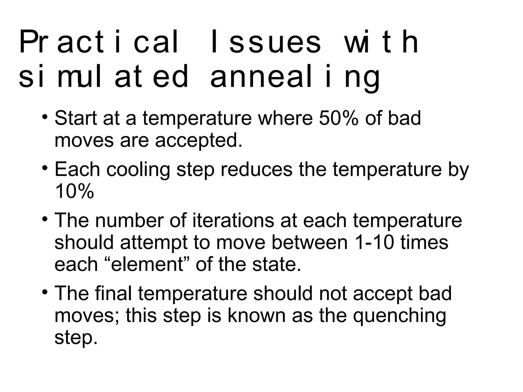
Call Girls in Nagpur Suman Call 7001035870 Meet With Nagpur Escorts
Simulated annealing presentation
1. Present ed by:
Amarendra Kumar Saroj ( Rol l
No: 182901)
Ram Kumar Basnet ( Rol l No: 182921)
ME Comput er Engi neeri ng [ III
Semest er]
Presentation on: Simulated Annealing (AI)
3. Local Search
al gori t hms
• Search algorithms like breadth-first, depth-first or
A* explore all the search space systematically by
keeping one or more paths in memory and by
recording which alternatives have been explored.
• When a goal is found, the path to that goal
constitutes a solution.
• Local search algorithms can be very helpful if we
are interested in the solution state but not in the
path to that goal. They operate only on the current
state and move into neighboring states .
4. Local Search
al gori t hms
• Local search algorithms have 2 key advantages:
• They use very little memory
• They can find reasonable solutions in large or
infinite (continuous) state spaces.
• Some examples of local search algorithms are:
• Hill-climbing
• Random walk
• Simulated annealing
5. Anneal i ng
• Annealing is a thermal process for obtaining low
energy states of a solid in a heat bath.
• The process contains two steps:
• Increase the temperature of the heat bath to a
maximum value at which the solid melts.
• Decrease carefully the temperature of the heat
bath until the particles arrange themselves in the
ground state of the solid. Ground state is a
minimum energy state of the solid.
• The ground state of the solid is obtained only if the
maximum temperature is high enough and the
cooling is done slowly.
6. Si mul at ed Anneal i ng
• The process of annealing can be simulated with
the Metropolis algorithm, which is based on Monte
Carlo techniques.
• We can apply this algorithm to generate a solution
to combinatorial optimization problems assuming
an analogy between them and physical many-
particle systems with the following equivalences:
• Solutions in the problem are equivalent to
states in a physical system.
• The cost of a solution is equivalent to the
“energy” of a state.
7. Si mul at ed Anneal i ng
• To apply simulated annealing with optimization purposes
we require the following:
• A successor function that returns a “close” neighboring
solution given the actual one. This will work as the
“disturbance” for the particles of the system.
• A target function to optimize that depends on the current
state of the system. This function will work as the energy
of the system.
• The search is started with a randomized state. In a polling
loop we will move to neighboring states always accepting
the moves that decrease the energy while only accepting
bad moves accordingly to a probability distribution
dependent on the “temperature” of the system.
10. Si mul at ed Anneal i ng: The
code
1. Create random initial solution γ
2. Eold=cost(γ);
3. for(temp=tempmax; temp>=tempmin;temp=next_temp(temp) ) {
4. for(i=0;i<imax; i++ ) {
5. succesor_func(γ); //this is a randomized function
6. Enew=cost(γ);
7. delta=Enew-Eold;
8. if(delta>0)
9. if(random() >= exp(-delta/K*temp);
10. undo_func(γ); //rejected bad move
11. else
12. Eold=Enew //accepted bad move
13. else
14. Eold=Enew; //always accept good moves
}
}
11. Si mul at ed Anneal i ng
• Acceptance criterion and cooling schedule
12. Pr act i cal I ssues wi t h
si mul at ed anneal i ng
• Cost function must be carefully developed, it has to
be “fractal and smooth”.
• The energy function of the left would work with SA
while the one of the right would fail.
13. Pr act i cal I ssues wi t h
si mul at ed anneal i ng
• The cost function should be fast it is going to be
called “millions” of times.
• The best is if we just have to calculate the deltas
produced by the modification instead of traversing
through all the state.
• This is dependent on the application.
14. Pr act i cal I ssues wi t h
si mul at ed anneal i ng
• In asymptotic convergence simulated annealing
converges to globally optimal solutions.
• In practice, the convergence of the algorithm
depends of the cooling schedule.
• There are some suggestion about the cooling
schedule but it stills requires a lot of testing and it
usually depends on the application.
15. • Start at a temperature where 50% of bad
moves are accepted.
• Each cooling step reduces the temperature by
10%
• The number of iterations at each temperature
should attempt to move between 1-10 times
each “element” of the state.
• The final temperature should not accept bad
moves; this step is known as the quenching
step.
Pr act i cal I ssues wi t h
si mul at ed anneal i ng
16. Appl i cat i ons
• Basic Problems
• Traveling salesman
• Graph partitioning
• Matching problems
• Graph coloring
• Scheduling
• Engineering
• VLSI design
• Placement
• Routing
• Array logic minimization
• Layout
• Facilities layout
• Image processing
• Code design in information theory