mechanical behaviour of material

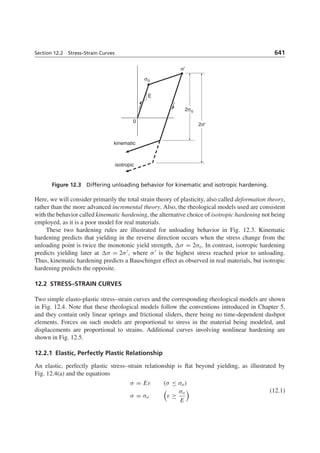
1. Section 12.2 Stress–Strain Curves 641
kinematic
isotropic
0
2σ'
2σo
σo
E
σ'
Figure 12.3 Differing unloading behavior for kinematic and isotropic hardening.
Here, we will consider primarily the total strain theory of plasticity, also called deformation theory,
rather than the more advanced incremental theory. Also, the rheological models used are consistent
with the behavior called kinematic hardening, the alternative choice of isotropic hardening not being
employed, as it is a poor model for real materials.
These two hardening rules are illustrated for unloading behavior in Fig. 12.3. Kinematic
hardening predicts that yielding in the reverse direction occurs when the stress change from the
unloading point is twice the monotonic yield strength, σ = 2σo. In contrast, isotropic hardening
predicts yielding later at σ = 2σ , where σ is the highest stress reached prior to unloading.
Thus, kinematic hardening predicts a Bauschinger effect as observed in real materials, but isotropic
hardening predicts the opposite.
12.2 STRESS–STRAIN CURVES
Two simple elasto-plastic stress–strain curves and the corresponding rheological models are shown
in Fig. 12.4. Note that these rheological models follow the conventions introduced in Chapter 5,
and they contain only linear springs and frictional sliders, there being no time-dependent dashpot
elements. Forces on such models are proportional to stress in the material being modeled, and
displacements are proportional to strains. Additional curves involving nonlinear hardening are
shown in Fig. 12.5.
12.2.1 Elastic, Perfectly Plastic Relationship
An elastic, perfectly plastic stress–strain relationship is flat beyond yielding, as illustrated by
Fig. 12.4(a) and the equations
σ = Eε (σ ≤ σo)
σ = σo ε ≥
σo
E
(12.1)

2. 642 Chapter 12 Plastic Deformation Behavior and Models for Materials
(a)
σσ
ε
E
o
σσ
ε
E
o
δE
(b)
σ
σ
εEo
σ
σ
εE
o
E2
1
0
0
Figure 12.4 Stress–strain curves and rheological models for (a) elastic, perfectly plastic
behavior and (b) elastic, linear-hardening behavior.
σ
σ
σ
σ
σ
ε
ε
ε
ε
ε = ε + ε
ε
ε ε
E
(a)
(b)
0
0
H
H
1
1
1
1
1
1
e
p
n
n(log)
(log)
E
ε
o
(log)
pe
, , ε (log)ε εpe
e p
σo
Figure 12.5 Stress–strain curves on linear and logarithmic coordinates for (a) an elastic,
power-hardening relationship and (b) the Ramberg–Osgood relationship.

3. Section 12.2 Stress–Strain Curves 643
where σo is the yield strength. This form is a reasonable approximation for the initial yielding
behavior of certain metals and other materials. Also, it is often used as a simple idealization to make
rough estimates, even where the stress–strain curve has a more complex shape.
Beyond yielding, the strain is the sum of elastic and plastic parts:
ε = εe + εp =
σ
E
+ εp ε >
σo
E
(12.2)
In the rheological model, the elastic strain εe is analogous to the deflection of the linear spring of
stiffness E, and the plastic strain εp is analogous to the movement of the frictional slider.
12.2.2 Elastic, Linear-Hardening Relationship
Elastic, linear-hardening behavior, Fig. 12.4(b), is useful as a rough approximation for stress–strain
curves that rise appreciably following yielding. Such a relationship requires an additional con-
stant, δ. This is the reduction factor for the slope following yielding, the slope before yielding
being the elastic modulus E and the one after yielding being δE. The value of δ can vary from zero
to unity, with smaller values giving flatter postyielding behavior. Also, δ = 0 gives a special case
that corresponds to the elastic, perfectly plastic relationship.
An equation for the postyield portion can be obtained by taking the slope between any point on
this part of the curve and the yield point:
δE =
σ − σo
ε − εo
(12.3)
Noting that the yield strain is given by εo = σo/E, and solving for stress, allows the entire
relationship to be specified:
σ = Eε (σ ≤ σo)
σ = (1 − δ) σo + δEε (σ ≥ σo)
(12.4)
It is sometimes convenient to solve the second equation for strain:
ε =
σo
E
+
(σ − σo)
δE
(σ ≥ σo) (12.5)
The response of the rheological model is the sum of the elastic strain in spring E1 and any
plastic strain in the spring–slider (E2, σo) parallel combination. No plastic strain occurs until the
stress exceeds the slider yield strength σo, and beyond this point the deflection of spring E2 is
also equal to the plastic strain. Noting that, beyond yielding, spring E2 is subjected to a stress of
(σ − σo), we can add the deflections in the two springs to obtain the total strain:
ε =
σ
E1
+
(σ − σo)
E2
(σ ≥ σo) (12.6)

4. 644 Chapter 12 Plastic Deformation Behavior and Models for Materials
Equations 12.5 and 12.6 are equivalent if the constants are related by
E = E1, δE =
E1 E2
E1 + E2
(12.7)
The slope δE corresponds to the stiffness of the two springs E1 and E2 in series.
12.2.3 Elastic, Power-Hardening Relationship
Reasonably accurate representation of the stress–strain curves of real materials generally requires
a more complex mathematical relationship than those described so far. One form that is sometimes
used assumes that stress is proportional to strain raised to a power, with this being applied only
beyond a yield strength σo:
σ = Eε (σ ≤ σo) (a)
σ = H1εn1 (σ ≥ σo) (b)
(12.8)
The term strain hardening exponent is used for n1, and H1 is an additional constant.
The most convenient means of fitting this relationship to a particular set of stress–strain data
is to make a log–log plot of stress versus strain, where for the postyield portion a straight line is
expected. This is illustrated on the right in Fig. 12.5(a). The value of σ at ε = 1 is H1. Assuming
that the logarithmic decades are the same length in both directions, we find that the slope of the line
is n1. On the same graph, the elastic region equation, σ = Eε, also forms a straight line, but with a
slope of unity, and the two lines intersect at σ = σo. Values of the exponent n1 are typically in the
range 0.05 to 0.4 for metals where this equation fits well.
Equation 12.8(b) can be easily expressed in terms of strain:
ε =
σ
H1
1/n1
(σ ≥ σo) (12.9)
Also, the yield strength is not an independent constant, as any two of σo, H1, and n1 may be
used to calculate the remaining one. An equation relating these can be obtained by applying both
Eqs. 12.8(a) and (b) at the point (εo, σo) and combining the results:
σo = E
H1
E
1/(1−n1)
(12.10)
12.2.4 Ramberg–Osgood Relationship
A relationship similar to that proposed in a report by Ramberg and Osgood in 1943 is frequently
used. Here, elastic and plastic strains, εe and εp, are considered separately and summed. An
exponential relationship is used, but it is applied to the plastic strain, rather than to the total strain
as before:
σ = Hεn
p (12.11)
This n is also called a strain hardening exponent, despite the fact that it is defined differently than
the previous n1.

5. Section 12.2 Stress–Strain Curves 645
Elastic strain is proportional to stress according to εe = σ/E, and plastic strain εp is the
deviation from the slope E, as shown in Fig. 12.5(b). Solving Eq. 12.11 for plastic strain and adding
the elastic and plastic strains gives an equation for total strain:
ε = εe + εp, ε =
σ
E
+
σ
H
1/n
(12.12)
This relationship cannot be solved explicitly for stress. It provides a single smooth curve for all
values of σ and does not exhibit a distinct yield point. Thus, it contrasts with the previously
described elastic, power-hardening form, which is discontinuous at a distinct yield point σo.
However, a yield strength may be defined as the stress corresponding to a given plastic strain offset,
such as εpo = 0.002, as in Fig. 4.11(a). Equation 12.11 then gives the offset yield strength:
σo = H(0.002)n
(12.13)
Constants for Eq. 12.12 for a particular set of stress–strain data are obtained by making a log–
log plot of stress versus plastic strain (σ versus εp), as illustrated on the right in Fig. 12.5(b). The
constant H is the value of σ at εp = 1, and n is the slope on the log–log plot if the logarithmic
decades in the two directions are of equal length. A plot of σ versus total strain ε is a curve on the
log–log plot. At small strains, this curve approaches the line of unity slope corresponding to elastic
strains; at large strains, it approaches the plastic strain line of slope n.
The Ramberg–Osgood equation and the power-hardening relationship are essentially equivalent
if the strains are sufficiently large that the plastic portion dominates, so that the elastic portion can
be considered to be negligible. The first term of Eq. 12.12 is then negligible, and values of H and n
fitted to data at large strains for ductile materials will be similar to values of H1 and n1 fitted to the
same data.
For tension tests, note that the Ramberg–Osgood form is often applied to true stresses and
strains, as already discussed in connection with Eq. 4.25.
Example 12.1
Some test data points on the monotonic stress–strain curve of 7075-T651 aluminum for uniaxial
stress are given in Table E12.1. Obtain values of the constants for a stress–strain curve of the
Ramberg–Osgood form, Eq. 12.12, that fits these data.
Solution The elastic modulus E is needed, as are the constants H and n. Prior to fitting, the
strains given as percentages need to be converted to dimensionless values, ε = ε%/100. Then,
plot all of the data on linear–linear coordinates as in Fig. E12.1(a), Curve 1. The overall trend
is a continuous curve that gradually deviates from an elastic slope, so that attempting a fit to
Eq. 12.12 is reasonable. The first three nonzero data points appear to form a straight line through
the origin, which is confirmed by plotting these on a sensitive strain scale (Curve 2). Fitting a
line σ = Eε gives an elastic modulus value that is rounded to E = 71,000 MPa.
We can now proceed to fit the constants H and n for the Eq. 12.11 relationship, σ = Hεn
p.
First, plastic strains εp are calculated for all of the data points where some nonlinearity is
apparent in Curve 1 of Fig. E12.1(a), using

6. 646 Chapter 12 Plastic Deformation Behavior and Models for Materials
Table E12.1
Test Data Calculations
Comment
σ, MPa ε, % ε εp log σ log εp
0 0 0 — — — Used for E
135.3 0.191 0.00191 — — — Used for E
270 0.381 0.00381 — — — Used for E
362 0.509 0.00509 — — — Used for E
406 0.576 0.00576 4.17 × 10−5
— — Not used
433 0.740 0.00740 0.001301 2.636 −2.886 Used for H, n
451 0.895 0.00895 0.002598 2.654 −2.585 Used for H, n
469 1.280 0.01280 0.006194 2.671 −2.208 Used for H, n
487 2.290 0.02290 0.01604 2.688 −1.795 Used for H, n
505 4.570 0.04570 0.03859 2.703 −1.414 Used for H, n
7075-T651 Al
σ = 71,013 ε
0
100
200
300
400
500
600
0.000 0.002 0.004 0.006 0.008 0.010
ε, Strain (Curve 2)
σ,Stress,MPa
0.00 0.01 0.02 0.03 0.04 0.05
ε, Strain (Curve 1)
Data, Curve 2
Data, Curve 1
Fit to R-O Eqn.
Fit E
Curve 1
Curve 2
Figure E12.1(a)
εp = ε −
σ
E
The resulting values are shown in Table E12.1. (Note that Eq. 12.12 implies that plastic strains
exist at all stress values. But at low stresses these become so small that they cannot be readily
measured in the laboratory, becoming essentially negligible.) Next, the stress versus plastic strain
data are plotted on log–log coordinates as shown in Fig. E12.1(b). The smallest εp value departs
from the linear trend of the other data and is so small that its accuracy is questionable; hence, this

7. Section 12.2 Stress–Strain Curves 647
7075-T651 Al
100
1000
εp, Plastic Strain
σ,Stress,MPa
Data fitted
Data rejected
Fit
10–5 10–210–310–4 10–1
σ = H ε
n
p
H = 585.5 MPa
n = 0.04453
Figure E12.1(b)
data point is rejected from the fitting process. The remaining data are then fitted to Eq. 12.11.
Taking logarithms of both sides of Eq. 12.11 gives
log σ = n log εp + log H
This is a straight line on a log–log plot; that is,
y = mx + b
where
y = log σ, x = log εp, m = n, b = log H
Performing a linear least-squares fit on this basis gives
m = n = 0.04453 Ans.
b = 2.7675, H = 10b
= 585.5 MPa Ans.
Discussion Equation 12.11 with the constants evaluated is thus
σ = 585.5ε0.04453
p MPa

8. 648 Chapter 12 Plastic Deformation Behavior and Models for Materials
The resulting straight line on a log–log plot of σ versus εp is shown in Fig. E12.1(b). Substituting
the constants obtained into Eq. 12.12 gives a relationship for the total strain:
ε =
σ
71,000
+
σ
585.5
1/0.04453
Here, σ is in units of MPa. Entering a number of values of σ into this equation and calculating
the corresponding total strains ε gives Curve 1 plotted in Fig. E12.1(a). The original data are in
good agreement with the fitted curve.
12.2.5 Rheological Modeling of Nonlinear Hardening
A stress–strain curve of either the elastic, power-hardening, or Ramberg–Osgood types can be
modeled by approximating it as a series of straight line segments, as illustrated in Fig. 12.6. The
first segment ends at the yield strength for the elastic, power-hardening case and at a low stress
where the plastic strain is small for the Ramberg–Osgood case. The corresponding rheological
model has a linear spring that gives an initial elastic slope, and then a series of spring and slider
parallel combinations that cause nonlinear behavior. The yield stresses for the various sliders have
δ
δ
δ
δ5
4
3
2E
E
E
E
E
0
σ
ε
σo5
σo5
σo4
σo4
σo3
σo3
σo2
σo2
E 2
E 3
E 4
E 5
E 1
σ
ε
Figure 12.6 Multistage spring and slider model for nonlinear-hardening stress–strain curves.