SlideShare a Scribd company logo
1 of 59
Download to read offline
4 146
Mechanics of Materials: Axial MembersM. VablePrintedfrom:http://www.me.mtu.edu/~mavable/MoM2nd.htm
August 2012
CHAPTER FOUR
AXIAL MEMBERS
Learning objectives
1. Understand the theory, its limitations, and its applications for the design and analysis of axial members.
2. Develop the discipline to draw free-body diagrams and approximate deformed shapes in the design and analysis of struc-
tures.
_______________________________________________
The tensile forces supporting the weight of the Mackinaw bridge (Figure 4.1a) act along the longitudinal axis of each cable. The
compressive forces raising the weight of the dump on a truck act along the axis of the hydraulic cylinders. The cables and
hydraulic cylinders are axial members, long straight bodies on which the forces are applied along the longitudinal axis.
Connecting rods in an engine, struts in aircraft engine mounts, members of a truss representing a bridge or a building, spokes
in bicycle wheels, columns in a building—all are examples of axial members
This chapter develops the simplest theory for axial members, following the logic shown in Figure 3.15 but subject to the
limitations described in Section 3,13. We can then apply the formulas to statically determinate and indeterminate structures.
The two most important tools in our analysis will be free-body diagrams and approximate deformed shapes.
4.1 PRELUDE TO THEORY
As a prelude to theory, we consider two numerical examples solved using the logic discussed in Section 3.2. Their solution
will highlight conclusions and observations that will be formalized in the development of the theory in Section 4.2.
Figure 4.1 Axial members: (a) Cables of Mackinaw bridge. (b) Hydraulic cylinders in a dump truck.
(a) (b)
4 147
Mechanics of Materials: Axial MembersM. VablePrintedfrom:http://www.me.mtu.edu/~mavable/MoM2nd.htm
August 2012
EXAMPLE 4.1
Two thin bars are securely attached to a rigid plate, as shown in Figure 4.2. The cross-sectional area of each bar is 20 mm2
. The force F
is to be placed such that the rigid plate moves only horizontally by 0.05 mm without rotating. Determine the force F and its location h for
the following two cases: (a) Both bars are made from steel with a modulus of elasticity E = 200 GPa. (b) Bar 1 is made of steel
(E = 200 GPa) and bar 2 is made of aluminum (E = 70 GPa).
PLAN
The relative displacement of point B with respect to A is 0.05 mm, from which we can find the axial strain. By multiplying the axial
strain by the modulus of elasticity, we can obtain the axial stress. By multiplying the axial stress by the cross-sectional area, we can
obtain the internal axial force in each bar. We can draw the free-body diagram of the rigid plate and by equilibrium obtain the force F and
its location h.
SOLUTION
1. Strain calculations: The displacement of B is uB = 0.05 mm. Point A is built into the wall and hence has zero displacement. The normal
strain is the same in both rods:
(E1)
2. Stress calculations: From Hooke’s law σ = Eε, we can find the normal stress in each bar for the two cases.
Case (a): Because E and ε1 are the same for both bars, the stress is the same in both bars. We obtain
(E2)
Case (b): Because E is different for the two bars, the stress is different in each bar
(E3)
(E4)
3. Internal forces: Assuming that the normal stress is uniform in each bar, we can find the internal normal force from N = σA, where
A = 20 mm2
= 20 × 10–6
m2
.
Case (a): Both bars have the same internal force since stress and cross-sectional area are the same,
(E5)
Case (b): The equivalent internal force is different for each bar as stresses are different.
(E6)
(E7)
4. External force: We make an imaginary cut through the bars, show the internal axial forces as tensile, and obtain free-body diagram
shown in Figure 4.3. By equilibrium of forces in x direction we obtain
(E8)
By equilibrium of moment point O in Figure 4.3, we obtain
(E9)
(E10)
Case (a): Substituting Equation (E5) into Equations (E8) and (E10), we obtain F and h:
ANS. F = 2000 N h = 10 mm
Case (b): Substituting Equations (E6) and (E7) into Equations (E8) and (E10), we obtain F and h:
200 mm
Bar 1
Bar 2
A
x
B
F
h 20 mm
Figure 4.2 Axial bars in Example 4.1.
ε1 ε2
uB uA–
xB xA–
------------------
0.05 mm
200 mm
--------------------- 250 μmm/mm= = = =
σ1 σ2 200 10
9
× N/m
2
( ) 250× 10
6–
× 50 10
6
× N/m
2
(T)= = =
σ1 E1ε1 200 10
9
× N/m
2
( ) 250× 10
6–
× 50 10
6
× N/m
2
(T)= = =
σ2 E2ε2 70 10
9
× 250 10
6–
×× 17.5 10
6
× N/m
2
(T)= = =
N1 N2 50 10
6
× N/m
2
( ) 20 10
6–
× m
2
( ) 1000 N (T)= = =
N1 σ1A1 50 10×
6
N/m
2
( ) 20 10
6–
× m
2
( ) 1000 N (T)= = =
N2 σ2A2 17.5 10×
6
N/m
2
( ) 20 10
6–
× m
2
( ) 350 N (T)= = =
F N1 N2+=
N1 20 h–( ) N2h– 0=
h
20N1
N1 N2+
--------------------=
FN1
N2NN
O
h 20 mm
Figure 4.3 Free-body diagram in Example 4.1.
F 1000 N 1000 N+ 2000 N= = h
20 mm 1000 N×
1000 N 1000 N+( )
----------------------------------------------- 10 mm= =
4 148
Mechanics of Materials: Axial MembersM. VablePrintedfrom:http://www.me.mtu.edu/~mavable/MoM2nd.htm
August 2012
ANS. F = 1350 N h = 14.81 mm
COMMENTS
1. Both bars, irrespective of the material, were subjected to the same axial strain. This is the fundamental kinematic assumption in the
development of the theory for axial members, discussed in Section 4.2.
2. The sum on the right in Equation (E8) can be written where σi is the normal stress in the ith bar, ΔAi is the cross-sec-
tional area of the ith bar, and n = 2 reflects that we have two bars in this problem. If we had n bars attached to the rigid plate, then the
total axial force would be given by summation over n bars. As we increase the number of bars n to infinity, the cross-sectional area
ΔAi tends to zero (or infinitesimal area dA) as we try to fit an infinite number of bars on the same plate, resulting in a continuous
body. The sum then becomes an integral, as discussed in Section 4.1.1.
3. If the external force were located at any point other than that given by the value of h, then the plate would rotate. Thus, for pure axial
problems with no bending, a point on the cross section must be found such that the internal moment from the axial stress distribution
is zero. To emphasize this, consider the left side of Equation (E9), which can be written as where yi is the coordinate
of the ith rod’s centroid. The summation is an expression of the internal moment that is needed for static equivalency. This internal
moment must equal zero if the problem is of pure axial deformation, as discussed in Section 4.1.1.
4. Even though the strains in both bars were the same in both cases, the stresses were different when E changed. Case (a) corresponds to
a homogeneous cross section, whereas case (b) is analogous to a laminated bar in which the non-homogeneity affects the stress distri-
bution.
4.1.1 Internal Axial Force
In this section we formalize the key observation made in Example 4.1: the normal stress σxx can be replaced by an equiva-
lent internal axial force using an integral over the cross-sectional area. Figure 4.4 shows the statically equivalent systems. The
axial force on a differential area σxx dA can be integrated over the entire cross section to obtain
(4.1)
If the normal stress distribution σxx is to be replaced by only an axial force at the origin, then the internal moments My and
Mz must be zero at the origin, and from Figure 4.4 we obtain
(4.2a)
(4.2b)
Equations (4.1), (4.2a), and (4.2b) are independent of the material models because they represent static equivalency
between the normal stress on the cross section and internal axial force. If we were to consider a laminated cross section or nonlin-
ear material, then it would affect the value and distribution of σxx across the cross section, but Equation (4.1) relating σxx and N
would remain unchanged, and so would the zero moment condition of Equations (4.2a) and (4.2b). Equations (4.2a) and (4.2b) are
used to determine the location at which the internal and external forces have to act for pure axial problem without bending, as dis-
cussed in Section 4.2.6.
F 1000 N 350 N+ 1350 N= = h
20 mm 1000 N×
1000 N 350 N+( )
-------------------------------------------- 14.81 mm= =
σi ΔAi,
i=1
n=2
∑
yiσi
ΔAi,
i=1
n
∑
N σxx Ad
A
∫=
x
y
y
dNdd ϭ ␴xx␴ dAx
O
z
Figure 4.4 Statically equivalent internal axial force.
O
x
y
N
yσxx Ad
A
∫ 0=
zσxx dA 0=
A
∫
4 149
Mechanics of Materials: Axial MembersM. VablePrintedfrom:http://www.me.mtu.edu/~mavable/MoM2nd.htm
August 2012
EXAMPLE 4.2
Figure 4.5 shows a homogeneous wooden cross section and a cross section in which the wood is reinforced with steel. The normal strain
for both cross sections is uniform, εxx = −200 μ. The moduli of elasticity for steel and wood are Esteel = 30,000 ksi and Ewood = 8000 ksi.
(a) Plot the σxx distribution for each of the two cross sections shown. (b) Calculate the equivalent internal axial force N for each cross
section using Equation (4.1).
PLAN
(a) Using Hooke’s law we can find the stress values in each material. Noting that the stress is uniform in each material, we can plot it
across the cross section. (b) For the homogeneous cross section we can perform the integration in Equation (4.1) directly. For the nonhomo-
geneous cross section we can write the integral in Equation (4.1) as the sum of the integrals over steel and wood and then perform the integra-
tion to find N.
SOLUTION
(a) From Hooke’s law we can write
(E1)
(E2)
For the homogeneous cross section the stress distribution is as given in Equation (E1), but for the laminated case it switches to Equation
(E2), depending on the location of the point where the stress is being evaluated, as shown in Figure 4.6.
(b) Homogeneous cross section: Substituting the stress distribution for the homogeneous cross section in Equation (4.1) and integrat-
ing, we obtain the equivalent internal axial force,
(E3)
ANS. N = 4.8 kips (C)
Laminated cross section: The stress value changes as we move across the cross section. Let Asb and Ast represent the cross-sectional
areas of steel at the bottom and the top. Let Aw represent the cross-sectional area of wood. We can write the integral in Equation (4.1) as
the sum of three integrals, substitute the stress values of Equations (E1) and (E2), and perform the integration:
or (E4)
or (E5)
(E6)
ANS. N = 9.2 kips (C)
Figure 4.5 Cross sections in Example 4.2. (a) Homogeneous. (b) Laminated.
y
z
2 in.
1
1
2
--- in.Wood
Steel
Wood
2 in.
Wood
Steel
Steel
y
z
1 in.
1/4 in.
1/4 in.
(a) (b)
σxx( )wood
8000 ksi( ) 200–( )10
6–
1.6 ksi–= =
σxx( )steel
30000 ksi( ) 200–( )10
6–
6 ksi–= =
(a)
6 ksi
(b)
6 ksi
1.6 ksi
Figure 4.6 Stress distributions in Example 4.2. (a) Homogeneous cross section. (b) Laminated cross section.
N σxx( )wood
Ad
A
∫ σxx( )wood
A 1.6 ksi–( ) 2 in.( ) 1.5 in.( ) 4.8– kips= = = =
N σxx A σxx A σxx Ad
Ast
∫+d
Aw
∫+d
Asb
∫ σxx( )steel
A σxx( )wood
A σxx( )steel
Ad
Ast
∫+d
Aw
∫+d
Asb
∫= =
N σxx( )steel
Asb σxx( )wood
Aw σxx( )steel
Ast+ +=
N 6 ksi–( ) 2 in.( )
1
4
--- in.
⎝ ⎠
⎛ ⎞ 1.6 ksi–( ) 1 in.( ) 2 in.( ) 6 ksi–( ) 2 in.( )
1
4
--- in.
⎝ ⎠
⎛ ⎞+ + 9.2– kips= =
4 150
Mechanics of Materials: Axial MembersM. VablePrintedfrom:http://www.me.mtu.edu/~mavable/MoM2nd.htm
August 2012
COMMENTS
1. Writing the integral in the internal axial force as the sum of integrals over each material, as in Equation (E4), is equivalent to calculat-
ing the internal force carried by each material and then summing, as shown in Figure 4.7.
2. The cross section is geometrically as well as materially symmetric. Thus we can locate the origin on the line of symmetry. If the lower
steel strip is not present, then we will have to determine the location of the equivalent force.
3. The example demonstrates that although the strain is uniform across the cross section, the stress is not. We considered material non-
homogeneity in this example. In a similar manner we can consider other models, such as elastic–perfectly plastic or material models
that have nonlinear stress–strain curves.
PROBLEM SET 4.1
4.1 Aluminum bars (E = 30,000 ksi) are welded to rigid plates, as shown in Figure P4.1. All bars have a cross-sectional area of 0.5 in2
. Due
to the applied forces the rigid plates at A, B, C, and D are displaced in x direction without rotating by the following amounts: uA = −0.0100 in., uB
= 0.0080 in., uC = −0.0045 in., and uD = 0.0075 in. Determine the applied forces F1, F2, F3, and F4.
4.2 Brass bars between sections A and B, aluminum bars between sections B and C, and steel bars between sections C and D are welded to
rigid plates, as shown in Figure P4.2. The rigid plates are displaced in the x direction without rotating by the following amounts: uB = −1.8 mm,
uC = 0.7 mm, and uD = 3.7 mm. Determine the external forces F1, F2, and F3 using the properties given in Table P4.2
4.3 The ends of four circular steel bars (E = 200 GPa) are welded to a rigid plate, as shown in Figure P4.3. The other ends of the bars are
built into walls. Owing to the action of the external force F, the rigid plate moves to the right by 0.1 mm without rotating. If the bars have a
diameter of 10 mm, determine the applied force F.
4.4 Rigid plates are securely fastened to bars A and B, as shown in Figure P4.4. A gap of 0.02 in. exists between the rigid plates before the
forces are applied. After application of the forces the normal strain in bar A was found to be 500 μ. The cross-sectional area and the modulus of
Figure 4.7 Statically equivalent internal force in Example 4.2 for laminated cross section.
6 ksi
6 ksi
F1 F4F
x
36 in 50 in 36 in
F2FF F3FF
F1 F4FF2FF F3FF
A B C D
FigureP4.1
F1 F2FF
F3FF
F3FF
F2FFF1
x
DCBA
1.5 m 2.5 m 2 mFigure P4.2
TABLE P4.2
Brass Aluminum Steel
Modulus of elasticity 70 GPa 100 GPa 200 GPa
Diameter 30 mm 25 mm 20 mm
1.5 m
F
F
2.5 m
Rigid plate
Figure P4.3
4 151
Mechanics of Materials: Axial MembersM. VablePrintedfrom:http://www.me.mtu.edu/~mavable/MoM2nd.htm
August 2012
elasticity for each bar are as follows: AA = 1 in.2
, EA = 10,000 ksi, AB = 0.5 in.2
, and EB = 30,000 ksi. Determine the applied forces F, assuming
that the rigid plates do not rotate.
4.5 The strain at a cross section shown in Figure P4.5 of an axial rod is assumed to have the uniform value εxx = 200 μ. (a) Plot the stress dis-
tribution across the laminated cross section. (b) Determine the equivalent internal axial force N and its location from the bottom of the cross
section. Use Ealu = 100 GPa, Ewood = 10 GPa, and Esteel = 200 GPa.
4.6 A reinforced concrete bar shown in Figure P4.6 is constructed by embedding 2-in. × 2-in. square iron rods. Assuming a uniform strain
εxx = −1500 μ in the cross section, (a) plot the stress distribution across the cross section; (b) determine the equivalent internal axial force N. Use
Eiron = 25,000 ksi and Econc = 3000 ksi.
4.2 THEORY OF AXIAL MEMBERS
In this section we will follow the procedure in Section 4.1 with variables in place of numbers to develop formulas for axial
deformation and stress. The theory will be developed subject to the following limitations:
1. The length of the member is significantly greater than the greatest dimension in the cross section.
2. We are away from the regions of stress concentration.
3. The variation of external loads or changes in the cross-sectional areas is gradual, except in regions of stress concentra-
tion.
4. The axial load is applied such that there is no bending.
5. The external forces are not functions of time that is, we have a static problem. (See Problems 4.37, 4.38, and 4.39 for
dynamic problems.)
Figure 4.8 shows an externally distributed force per unit length p(x) and external forces F1 and F2 acting at each end of an
axial bar. The cross-sectional area A(x) can be of any shape and could be a function of x.
Sign convention: The displacement u is considered positive in the positive x direction. The internal axial
force N is considered positive in tension negative in compression.
Bar A
Bar B
Bar A
Bar B
in
0.02 in
F
F
60 in
Rigid plates
Figure P4.4
Figure P4.5
80 mm
100 mm
10 mm
Aluminum
10 mm
Steel
Wood
z
x
y
z
x
y 4 i
4 i
4 in 4 inFigure P4.6
4 152
Mechanics of Materials: Axial MembersM. VablePrintedfrom:http://www.me.mtu.edu/~mavable/MoM2nd.htm
August 2012
The theory has two objectives:
1. To obtain a formula for the relative displacements u2 − u1 in terms of the internal axial force N.
2. To obtain a formula for the axial stress σxx in terms of the internal axial force N.
We will take Δx = x2 − x1 as an infinitesimal distance so that the gradually varying distributed load p(x) and the cross-sec-
tional area A(x) can be treated as constants. We then approximate the deformation across the cross section and apply the logic
shown in Figure 4.9. The assumptions identified as we move from each step are also points at which complexities can later be
added, as discussed in examples and “Stretch Yourself” problems.
4.2.1 Kinematics
Figure 4.10 shows a grid on an elastic band that is pulled in the axial direction. The vertical lines remain approximately vertical, but
the horizontal distance between the vertical lines changes. Thus all points on a vertical line are displaced by equal amounts. If this
surface observation is also true in the interior of an axial member, then all points on a cross-section displace by equal amounts, but
each cross-section can displace in the x direction by a different amount, leading to Assumption 1.
Figure 4.8 Segment of an axial bar.
u2
u1
x
y
z
x1
F2FF
x2
Figure 4.9 Logic in mechanics of materials.
x
y
(a) (b)
Figure 4.10 Axial deformation: (a) original grid; (b) deformed grid. (c) u is constant in y direction.
(c)
4 153
Mechanics of Materials: Axial MembersM. VablePrintedfrom:http://www.me.mtu.edu/~mavable/MoM2nd.htm
August 2012
Assumption 1 Plane sections remain plane and parallel.
Assumption 1 implies that u cannot be a function of y but can be a function of x
(4.3)
As an alternative perspective, because the cross section is significantly smaller than the length, we can approximate a function
such as u by a constant treating it as uniform over a cross section. In Chapter 6, on beam bending, we shall approximate u as a linear
function of y.
4.2.2 Strain Distribution
Assumption 2 Strains are small.1
If points x2 and x1 are close in Figure 4.8, then the strain at any point x can be calculated as
or
(4.4)
Equation (4.4) emphasizes that the axial strain is uniform across the cross section and is only a function of x. In deriving Equa-
tion (4.4) we made no statement regarding material behavior. In other words, Equation (4.4) does not depend on the material
model if Assumptions 1 and 2 are valid. But clearly if the material or loading is such that Assumptions 1 and 2 are not tenable,
then Equation (4.4) will not be valid.
4.2.3 Material Model
Our motivation is to develop a simple theory for axial deformation. Thus we make assumptions regarding material behavior that
will permit us to use the simplest material model given by Hooke’s law.
Assumption 3 Material is isotropic.
Assumption 4 Material is linearly elastic.2
Assumption 5 There are no inelastic strains.3
Substituting Equation (4.4) into Hooke’s law, that is, we obtain
(4.5)
Though the strain does not depend on y or z, we cannot say the same for the stress in Equation (4.5) since E could change across the
cross section, as in laminated or composite bars.
4.2.4 Formulas for Axial Members
Substituting σxx from Equation (4.5) into Equation (4.1) and noting that du/dx is a function of x only, whereas the integration
is with respect to y and z (dA = dy dz), we obtain
(4.6)
1
See Problem 4.40 for large strains.
2
See Problem 4.36 for nonlinear material behavior.
3
Inelastic strains could be due to temperature, humidity, plasticity, viscoelasticity, and so on. We shall consider inelastic strains due to tem-
perature in Section 4.5.
u u x( )=
εxx Δx 0→
lim
u2 u1–
x2 x1–
-----------------
⎝ ⎠
⎛ ⎞
Δx 0→
lim
Δu
Δx
-------
⎝ ⎠
⎛ ⎞= =
εxx
du
dx
------ x( )=
σxx E εxx,=
σxx E
du
dx
------=
N E
du
dx
------ Ad
A
∫
du
dx
------ E dA
A
∫= =
4 154
Mechanics of Materials: Axial MembersM. VablePrintedfrom:http://www.me.mtu.edu/~mavable/MoM2nd.htm
August 2012
Consistent with the motivation for the simplest possible formulas, E should not change across the cross section as implied in
Assumption 6. We can take E outside the integral.
Assumption 6 Material is homogeneous across the cross section.
With material homogeneity, we then obtain
or
(4.7)
The higher the value of EA, the smaller will be the deformation for a given value of the internal force. Thus the rigidity of
the bar increases with the increase in EA. This implies that an axial bar can be made more rigid by either choosing a stiffer mate-
rial (a higher value of E) or increasing the cross-sectional area, or both. Example 4.5 brings out the importance of axial rigidity
in design. The quantity EA is called axial rigidity.
Substituting Equation (4.7) into Equation (4.5), we obtain
(4.8)
In Equation (4.8), N and A do not change across the cross section and hence axial stress is uniform across the cross section.
We have used Equation (4.8) in Chapters 1 and 3, but this equation is valid only if all the limitations are imposed, and if Assump-
tions 1 through 6 are valid.
We can integrate Equation (4.7) to obtain the deformation between two points:
(4.9)
where u1 and u2 are the displacements of sections at x1 and x2, respectively. To obtain a simple formula we would like to take the
three quantities N, E, and A outside the integral, which means these quantities should not change with x. To achieve this simplicity,
we make the following assumptions:
Assumption 7 The material is homogeneous between x1 and x2. (E is constant)
Assumption 8 The bar is not tapered between x1 and x2. (A is constant)
Assumption 9 The external (hence internal) axial force does not change with x between x1 and x2. (N is constant)
If Assumptions 7 through 9 are valid, then N, E, and A are constant between x1 and x2, and we obtain
(4.10)
In Equation (4.10), points x1 and x2 must be chosen such that neither N, E, nor A changes between these points.
4.2.5 Sign Convention for Internal Axial Force
The axial stress σxx was replaced by a statically equivalent internal axial force N. Figure 4.11 shows the sign convention for
the positive axial force as tension.
N is an internal axial force that has to be determined by making an imaginary cut and drawing a free-body diagram. In what
direction should N be drawn on the free-body diagram? There are two possibilities:
1. N is always drawn in tension on the imaginary cut as per our sign convention. The equilibrium equation then gives a
positive or a negative value for N. A positive value of σxx obtained from Equation (4.8) is tensile and a negative value is
N E
xd
du
Ad
A
∫ EA
xd
du
= =
xd
du N
EA
-------=
σxx
N
A
----=
u2 u1– ud
u1
u2
∫
N
EA
-------
x1
x2
∫ dx= =
u2 u1–
N x2 x1–( )
EA
--------------------------=
ϩNFigure 4.11 Sign convention for positive internal axial force.
4 155
Mechanics of Materials: Axial MembersM. VablePrintedfrom:http://www.me.mtu.edu/~mavable/MoM2nd.htm
August 2012
compressive. Similarly, the relative deformation obtained from Equation (4.10) is extension for positive values and con-
traction for negative values. The displacement u will be positive in the positive x direction.
2. N is drawn on the imaginary cut in a direction to equilibrate the external forces. Since inspection is being used in
determining the direction of N, tensile and compressive σxx and extension or contraction for the relative deformation
must also be determined by inspection.
4.2.6 Location of Axial Force on the Cross Section
For pure axial deformation the internal bending moments must be zero. Equations (4.2a) and (4.2b) can then be used to deter-
mine the location of the point where the internal axial force and hence the external forces must pass for pure axial problems.
Substituting Equation (4.5) into Equations (4.2a) and (4.2b) and noting that du/dx is a function of x only, whereas the integration
is with respect to y and z (dA = dy dz), we obtain
or
(4.11a)
or
(4.11b)
Equations (4.11a) and (4.11b) can be used to determine the location of internal axial force for composite materials. If the
cross section is homogenous (Assumption 6), then E is constant across the cross section and can be taken out side the integral:
(4.12a)
(4.12b)
Equations (4.12a) and (4.12b) are satisfied if y and z are measured from the centroid. (See Appendix A.4.) We will have pure
axial deformation if the external and internal forces are colinear and passing through the centroid of a homogenous cross sec-
tion. This assumes implicitly that the centroids of all cross sections must lie on a straight line. This eliminates curved but not
tapered bars.
4.2.7 Axial Stresses and Strains
In the Cartesian coordinate system all stress components except σxx are assumed zero. From the generalized Hooke’s law for iso-
tropic materials, given by Equations (3.14a) through (3.14c), we obtain the normal strains for axial members:
(4.13)
where ν is the Poisson’s ratio. In Equation (4.13), the normal strains in y and z directions are due to Poisson’s effect. Assumption 1,
that plane sections remain plane and parallel implies that no right angle would change during deformation, and hence the assumed
deformation implies that shear strains in axial members are zero. Alternatively, if shear stresses are zero, then by Hooke’s law shear
strains are zero.
yσxx Ad
A
∫ yE
du
dx
------ Ad
A
∫
du
dx
------ yE Ad
A
∫ 0= = =
yE Ad
A
∫ 0=
zσxx dA zE
du
dx
------ Ad
A
∫=
A
∫
du
dx
------ zE Ad
A
∫ 0= =
zE Ad
A
∫ 0=
y Ad
A
∫ 0=
z Ad
A
∫ 0=
εxx
σxx
E
-------- εyy
νσxx
E
-----------–= νεxx εzz
νσxx
E
-----------–=– νεxx–= = =
4 156
Mechanics of Materials: Axial MembersM. VablePrintedfrom:http://www.me.mtu.edu/~mavable/MoM2nd.htm
August 2012
EXAMPLE 4.3
Solid circular bars of brass (Ebr = 100 GPa, νbr = 0.34) and aluminum (Eal = 70 GPa, νal = 0.33) having 200 mm diameter are attached to
a steel tube (Est = 210 GPa, νst = 0.3) of the same outer diameter, as shown in Figure 4.12. For the loading shown determine: (a) The
movement of the plate at C with respect to the plate at A. (b) The change in diameter of the brass cylinder. (c) The maximum inner diam-
eter to the nearest millimeter in the steel tube if the factor of safety with respect to failure due to yielding is to be at least 1.2. The yield
stress for steel is 250 MPa in tension.
PLAN
(a) We make imaginary cuts in each segment and determine the internal axial forces by equilibrium. Using Equation (4.10) we can find
the relative movements of the cross sections at B with respect to A and at C with respect to B and add these two relative displacements to
obtain the relative movement of the cross section at C with respect to the section at A. (b) The normal stress σxx in AB can be obtained
from Equation (4.8) and the strain εyy found using Equation (4.13). Multiplying the strain by the diameter we obtain the change in diam-
eter. (c) We can calculate the allowable axial stress in steel from the given failure values and factor of safety. Knowing the internal force in
CD we can find the cross-sectional area from which we can calculate the internal diameter.
SOLUTION
(a) The cross-sectional areas of segment AB and BC are
(E1)
We make imaginary cuts in segments AB, BC, and CD and draw the free-body diagrams as shown in Figure 4.13. By equilibrium of
forces we obtain the internal axial forces
(E2)
We can find the relative movement of point B with respect to point A, and C with respect to B using Equation (4.10):
(E3)
(E4)
Adding Equations (E3) and (E4) we obtain the relative movement of point C with respect to A:
(E5)
ANS. uC − uA = 0.7845 mm contraction
(b) We can find the axial stress σxx in AB using Equation (4.8):
(E6)
Substituting σxx, Ebr = 100 GPa, νbr = 0.34 in Equation (4.13), we can find εyy. Multiplying εyy by the diameter of 200 mm, we then obtain
the change in diameter Δd,
(E7)
ANS. Δd = −0.032 mm
(c) The axial stress in segment CD is
Figure 4.12 Axial member in Example 4.3.
2000 kN
2000 kN
2750 kN
2750 kN
1500 kN
1500 kN
750 kN
750 kN
A
x
0.5 m 1.5 m 0.6 m
AAB ABC
π
4
--- 0.2 m( )
2
31.41 10×
3–
m
2
= = =
NAB 1500 kN= NBC 1500 kN 3000 kN– 1500 kN–= = NCD 4000 kN= =
750 kN
750 kN
NABN
Figure 4.13 Free body diagrams in Example 4.3.
NBCN
750 kN
750 kN
1500 kN
1500 kN
NCD
2000 kN
2000 kN
(a) (b) (c)
uB uA
NAB xB xA–( )
EABAAB
---------------------------------=–
1500 10
3
× N( ) 0.5 m( )
100 10
9
× N/m
2
( ) 31.41 10×
3–
m
2
( )
----------------------------------------------------------------------------------------- 0.2388 10
3–
× m= =
uC uB–
NBC xC xB–( )
EBCABC
---------------------------------
1500– 10×
3
N( ) 1.5 m( )
70 10×
9
N/m
2
( ) 31.41 10×
3–
m
2
( )
-------------------------------------------------------------------------------------- 1.0233 10
3–
×– m= = =
uC uA– uC uB–( ) uB uA–( )+ 0.2388 m 1.0233 m–( )10
3–
0.7845 10
3–
× m–= = =
σxx
NAB
AAB
----------
1500 10×
3
N
31.41 10×
3–
m
2
( )
--------------------------------------------- 47.8 10×
6
N/m
2
= = =
εyy
νbrσxx
Ebr
---------------–
0.34 47.8 10×
6
N/m
2
( )
100 10× 9 N/m
2
--------------------------------------------------------– 0.162 10×
3–
–= =
Δd
200 mm
--------------------= =
4 157
Mechanics of Materials: Axial MembersM. VablePrintedfrom:http://www.me.mtu.edu/~mavable/MoM2nd.htm
August 2012
(E8)
Using the given factor of safety, we determine the value of Di:
or
(E9)
To the nearest millimeter, the diameter that satisfies the inequality in Equation (E9) is 124 mm.
ANS. Di = 124 mm
COMMENTS
1. On a free-body diagram some may prefer to show N in a direction that counterbalances the external forces, as shown in Figure 4.14.
In such cases the sign convention is not being followed.
We note that uB− uA = 0.2388 (10−3
) m is extension and uC − uB = 1.0233 (10−3
) m is contraction. To calculate uC − uA we must now manu-
ally subtract uC − uB from uB− uA .
2. An alternative way of calculating of uC − uA is
or, written more compactly,
(4.14)
where n is the number of segments on which the summation is performed, which in our case is 2. Equation (4.14) can be used only if the
sign convention for the internal force N is followed.
3. Note that NBC − NAB = −3000 kN and the magnitude of the applied external force at the section at B is 3000 kN. Similarly, NCD − NBC
= 5500 kN, which is the magnitude of the applied external force at the section at C. In other words, the internal axial force jumps by
the value of the external force as one crosses the external force from left to right. We will make use of this observation in the next sec-
tion, when we develop a graphical technique for finding the internal axial force.
4.2.8 Axial Force Diagram
In Example 4.3 we constructed several free-body diagrams to determine the internal axial force in different segments of the axial
member. An axial force diagram is a graphical technique for determining internal axial forces, which avoids the repetition of
drawing free-body diagrams.
An axial force diagram is a plot of the internal axial force N versus x. To construct an axial force diagram we create a small
template to guide us in which direction the internal axial force will jump, as shown in Figure 4.15a and Figure 4.15b. An axial
template is a free-body diagram of a small segment of an axial bar created by making an imaginary cut just before and just after
the section where the external force is applied.
σCD
NCD
ACD
-----------
4000 10
3
× N
π 4⁄( ) 0.2 m( )
2
Di
2
–[ ]
------------------------------------------------------
16,000 10
3
×
π 0.2
2
Di
2
–( )[ ]
------------------------------------ N/m
2
= = =
K
σyield
σCD
-------------
250 10
6
π 0.2
2
Di
2
–( )[ ]××
16,000 10
3
×
------------------------------------------------------------------ 49.09 0.2
2
Di
2
–( ) 1.2≥= = =
Di
2
0.2
2
24.45 10
3–
×–≤ or Di 124.7 10
3–
× m≤
NBCN
1500 kN
1500 kN
750 kN
750 kN
(b)
NABN
750 kN
750 kN
(a)
Figure 4.14 Alternative free body diagrams in Example 4.3.
uC uA–
N
EA
------- dx
xA
xC
∫
NAB
EABAAB
-------------------- dx
NBC
EBCABC
-------------------- dx
xB
xC
∫+
xA
xB
∫= =
uC uB–
⎫
⎬
⎭
uB uA–⎫
⎬
⎭
Δu
Ni Δxi
EiAi
---------------
i 1=
n
∑=
N1 N2NN
FextFF
2
FextF
2
Figure 4.15 Axial bar templates. N2 = N1 − Fext
(a)
N1
N2NN
FextF
2
FextFF
2
N2 = N1 + Fextt
(b)
Template Equations
4 158
Mechanics of Materials: Axial MembersM. VablePrintedfrom:http://www.me.mtu.edu/~mavable/MoM2nd.htm
August 2012
The external force Fext on the template can be drawn either to the left or to the right. The ends represent the imaginary cut
just to the left and just to the right of the applied external force. On these cuts the internal axial forces are drawn in tension. An
equilibrium equation—that is, the template equation—is written as shown in Figure 4.15 If the external force on the axial bar is
in the direction of the assumed external force on the template, then the value of N2 is calculated according to the template equa-
tion. If the external force on the axial bar is opposite to the direction shown on the template, then N2 is calculated by changing
the sign of Fext in the template equation. Example 4.4 demonstrates the use of templates in constructing axial force diagrams.
EXAMPLE 4.4
Draw the axial force diagram for the axial member shown in Example 4.3 and calculate the movement of the section at C with respect to
the section at A.
PLAN
We can start the process by considering an imaginary extension on the left. In the imaginary extension the internal axial force is zero.
Using the template in Figure 4.15a to guide us, we can draw the axial force diagram. Using Equation (4.14), we can find the relative dis-
placement of the section at C with respect to the section at A.
SOLUTION
Let LA be an imaginary extension on the left of the shaft, as shown in Figure 4.16a. Clearly the internal axial force in the imaginary segment
LA is zero. As one crosses the section at A, the internal force must jump by the applied axial force of 1500 kN. Because the forces at A are in the
opposite direction to the force Fext shown on the template in Figure 4.15a, we must use opposite signs in the template equation. The internal
force just after the section at A will be +1500 kN. This is the starting value in the internal axial force diagram.
We approach the section at B with an internal force value of +1500 kN. The force at B is in the same direction as the force shown on the
template in Figure 4.15a. Hence we subtract 3000 as per the template equation, to obtain a value of −1500 kN, as shown in Figure 4.16b.
We now approach the section at C with an internal force value of −1500 kN and note that the forces at C are opposite to those on the tem-
plate in Figure 4.15a. Hence we add 5500 to obtain +4000 kN.
The force at D is in the same direction as that on the template in Figure 4.15a, and after subtracting we obtain a zero value in the imagi-
nary extended bar DR. The return to zero value must always occur because the bar is in equilibrium.
From Figure 4.16b the internal axial forces in segments AB and BC are NAB = 1500 kN and NBC = −1500 kN. The crosssectional areas as calcu-
lated in Example 4.3 are and modulas of elasticity for the two sections are EAB = 100 GPa and EBC= 70
GPa. Substituting these values into Equation (4.14) we obtain the relative deformation of the section at C with respect to the section at A,
(E1)
or (E2)
ANS. uC − uA = 0.7845 mm contraction
COMMENT
1. We could have used the template in Figure 4.15b to create the axial force diagram.We approach the section at A and note that the +1500
kN is in the same direction as that shown on the template of Figure 4.15b. As per the template equation we add. Thus our starting value
is +1500 kN, as shown in Figure 4.16. As we approach the section at B, the internal force N1 is +1500 kN, and the applied force of 3000
kN is in the opposite direction to the template of Figure 4.15b, so we subtract to obtain N2 as –1500 kN. We approach the section at C
and note that the applied force is in the same direction as the applied force on the template of Figure 4.15b. Hence we add 5500 kN to
obtain +4000 kN. The force at section D is opposite to that shown on the template of Figure 4.15b, so we subtract 4000 to get a zero
value in the extended portion DR. The example shows that the direction of the external force Fext on the template is immaterial.
2000 kN
2000 kN
2750 kN
2750 kN
1500 kN
1500 kN
750 kN
750 kN
A
L R
0.5 m 1.5 m 0.6 m
Figure 4.16 (a) Extending the axial bar for an axial force diagram. (b) Axial force diagram.
N (kN)N
A
B C D
4000
1500
Ϫ1500
x
(a) (b)
AAB ABC 31.41 10×
3–
m
2
= =
Δu uC uA–
NAB xB xA–( )
EABAAB
---------------------------------
NBC xC xB–( )
EBCABC
---------------------------------+= =
uC uA–
1500 10× 3 N( ) 0.5 m( )
100 10× 9 N/m
2
( ) 31.41 10×
3–
m
2
( )
-----------------------------------------------------------------------------------------
1500– 10× 3 N( ) 1.5 m( )
70 109× N/m
2
( ) 31.41 10×
3–
m
2
( )
--------------------------------------------------------------------------------------+ 0.7845 10
3–
× m–= =
4 159
Mechanics of Materials: Axial MembersM. VablePrintedfrom:http://www.me.mtu.edu/~mavable/MoM2nd.htm
August 2012
EXAMPLE 4.5
A 1-m-long hollow rod is to transmit an axial force of 60 kN. Figure 4.17 shows that the inner diameter of the rod must be 15 mm to fit
existing attachments. The elongation of the rod is limited to 2.0 mm. The shaft can be made of titanium alloy or aluminum. The modulus
of elasticity E, the allowable normal stress σallow, and the density γ for the two materials is given in Table 4.1. Determine the minimum
outer diameter to the nearest millimeter of the lightest rod that can be used for transmitting the axial force.
PLAN
The change in radius affects only the cross-sectional area A and no other quantity in Equations (4.8) and (4.10). For each material we can
find the minimum cross-sectional area A needed to satisfy the stiffness and strength requirements. Knowing the minimum A for each
material, we can find the minimum outer radius. We can then find the volume and hence the mass of each material and make our decision
on the lighter bar.
SOLUTION
We note that for both materials x2 – x1 = 1 m. From Equations (4.8) and (4.10) we obtain for titanium alloy the following limits on ATi:
(E1)
(E2)
Using similar calculations for the aluminum shaft, we obtain the following limits on AAl:
(E3)
(E4)
Thus if , it will meet both conditions in Equations (E1) and (E2). Similarly if , it will
meet both conditions in Equations (E3) and (E4). The external diameters DTi and DAl are then
(E5)
(E6)
Rounding upward to the closest millimeter, we obtain
(E7)
We can find the mass of each material by taking the product of the material density and the volume of a hollow cylinder,
(E8)
(E9)
From Equations (E8) and (E9) we see that the titanium alloy shaft is lighter.
ANS. A titanium alloy shaft with an outside diameter of 25 mm should be used.
COMMENTS
1. For both materials the stiffness limitation dictated the calculation of the external diameter, as can be seen from Equations (E1) and
(E3).
1 m
15 mm
Figure 4.17 Cylindrical rod in Example 4.5.
TABLE 4.1 Material properties in Example 4.4
Material
E
(GPa)
σallow
(MPa)
γ
(mg/m3
)
Titanium alloy 96 400 4.4
Aluminum 70 200 2.8
Δu( )Ti
60 10×
3
N( ) 1 m( )
96 10×
9
N/m
2
( )ATi
------------------------------------------------- 2 10
3–
m×≤= or ATi 0.313 10×
3–
m
2
≥
σmax( )Ti
60 10×
3
N( )
ATi
------------------------------- 400 10×
6
N/m
2
≤= or ATi 0.150 10×
3–
m
2
≥
Δu( )Al
60 10×
3
N( ) 1×
28 10×
9
N/m
2
( )AAl
------------------------------------------------- 2 10×
3–
m≤= or AAl 1.071 10×
3–
m
2
≥
σmax( )Al
60 10×
3
N( )
AAl
------------------------------- 200 10×
6
N/m
2
≤= or AAl 0.300 10×
3–
m
2
≥
ATi 0.313 10×
3–
m
2
≥ AAl 1.071 10
3–
× m
2
≥
ATi
π
4
--- DTi
2
0.015
2
–( ) 0.313 10×
3–
≥= DTi 24.97 10×
3–
m≤
AAl
π
4
--- DAl
2
0.015
2
–( ) 1.071 10×
3–
≥= DAl 39.86 10
3–
× m≤
DTi 25 10
3–
( ) m= DAl 40 10
3–
( ) m=
mTi 4.4 10×
6
g/m
3
( )
π
4
--- 0.025
2
0.015
2
–( ) m
2
⎩ ⎭
⎨ ⎬
⎧ ⎫
1 m( ) 1382 g= =
mAl 2.8 10
6
× g/m
3
( )
π
4
--- 0.040
2
0.015
2
–( ) m
2
⎩ ⎭
⎨ ⎬
⎧ ⎫
1 m( ) 3024 g= =
4 160
Mechanics of Materials: Axial MembersM. VablePrintedfrom:http://www.me.mtu.edu/~mavable/MoM2nd.htm
August 2012
2. Even though the density of aluminum is lower than that of titanium alloy, the mass of titanium is less. Because of the higher modulus
of elasticity of titanium alloy, we can meet the stiffness requirement using less material than with aluminum.
3. The answer may change if cost is a consideration. The cost of titanium per kilogram is significantly higher than that of aluminum.
Thus based on material cost we may choose aluminum. However, if the weight affects the running cost, then economic analysis is
needed to determine whether the material cost or the running cost is higher.
4. If in Equation (E5) we had 24.05 × 10⁻³
m on the right-hand side, our answer for DTi would still be 25 mm because we have to round
upward to ensure meeting the greater-than sign requirement in Equation (E5).
EXAMPLE 4.6
A rectangular aluminum bar (Eal = 10,000 ksi, ν = 0.25) of -in. thickness consists of a uniform and tapered cross section, as shown in
Figure 4.18. The depth in the tapered section varies as h(x) = (2 − 0.02x) in. Determine: (a) The elongation of the bar under the applied
loads. (b) The change in dimension in the y direction in section BC.
PLAN
(a) We can use Equation (4.10) to find uC − uB. Noting that cross-sectional area is changing with x in segment AB, we integrate Equation
(4.7) to obtain uB − uA. We add the two relative displacements to obtain uC − uA and noting that uA = 0 we obtain the extension as uC. (b)
Once the axial stress in BC is found, the normal strain in the y direction can be found using Equation (4.13). Multiplying by 2 in., the
original length in the y direction, we then find the change in depth.
SOLUTION
The cross-sectional areas of AB and BC are
(E1)
(a) We can make an imaginary cuts in segment AB and BC, to obtain the free-body diagrams in Figure 4.19. By force equilibrium we
obtain the internal forces,
(E2)
The relative movement of point C with respect to point B is
(E3)
Equation (4.7) for segment AB can be written as
(E4)
Integrating Equation (E4), we obtain the relative displacement of B with respect to A:
or
(E5)
We obtain the relative displacement of C with respect to A by adding Equations (E3) and (E5):
(E6)
We note that point A is fixed to the wall, and thus uA = 0.
ANS. uC = 0.036 in. elongation
(b) The axial stress in BC is σAB = NBC /ABC = 10/1.5 = 6.667 ksi. From Equation (4.13) the normal strain in y direction can be found,
3
4
---
y
P
50 in 20 in
3
4 in
4 in
Figure 4.18 Axial member in Example 4.6.
ABC
3
4
--- in.
⎝ ⎠
⎛ ⎞ 2 in.( ) 1.5 in.
2
= = AAB
3
4
--- in.
⎝ ⎠
⎛ ⎞ 2h in.( ) 1.5 2 0.02x–( ) in.
2
= =
10 kipsNBCN
Figure 4.19 Free-body diagrams in Example 4.6.
10 kipsNABN
NAB 10 kips= NBC 10 kips=
uC uB–
NBC xC xB–( )
EBCABC
---------------------------------
10 kips( ) 20 in.( )
10,000 ksi( ) 1.5 in.
2
( )
------------------------------------------------------ 13.33 10
3–
× in.= = =
xd
du
⎝ ⎠
⎛ ⎞
AB
NAB
EABAAB
--------------------
10 kips
10,000 ksi( ) 1.5 2 0.02x–( ) in.
2
[ ]
---------------------------------------------------------------------------------= =
du
uA
uB
∫
10
3–
1.5 2 0.02x–( )
----------------------------------- dx
xA=0
xB=50
∫ in.=
uB uA–
10
3–
1.5
-----------
1
0.02–( )
------------------ 2 0.02x–( )ln
0
50
10
3–
0.03
----------- 1( ) 2( )ln–ln[ ] in.– 23.1 10×
3–
in.= = =
uC uA– 13.33 10
3–
× 23.1 10×
3–
+ 36.43 10
3–
× in.= =
4 161
Mechanics of Materials: Axial MembersM. VablePrintedfrom:http://www.me.mtu.edu/~mavable/MoM2nd.htm
August 2012
(E7)
The change in dimension in the y direction Δv can be found as
(E8)
ANS. Δv = 0.3333 × 10⁻³
in. contraction
COMMENT
1. An alternative approach is to integrate Equation (E4):
(E9)
To find constant of integration c, we note that at x = 0 the displacement u = 0. Hence, c = (10−3
/0.03) ln (2). Substituting the value, we
obtain
(E10)
Knowing u at all x, we can obtain the extension by substituting x = 50 to get the displacement at C.
EXAMPLE 4.7
The radius of a circular truncated cone in Figure 4.20 varies with x as R(x) = (r/L)(5L − 4x). Determine the extension of the truncated cone
due to its own weight in terms of E, L, r, and γ, where E and γ are the modulus of elasticity and the specific weight of the material,
respectively.
PLAN
We make an imaginary cut at location x and take the lower part of the truncated cone as the free-body diagram. In the free-body diagram
we can find the volume of the truncated cone as a function of x. Multiplying the volume by the specific weight, we can obtain the weight
of the truncated cone and equate it to the internal axial force, thus obtaining the internal force as a function of x. We then integrate Equa-
tion (4.7) to obtain the relative displacement of B with respect to A.
SOLUTION
Figure 4.21 shows the free-body diagram after making a cut at some location x. We can find the volume V of the truncated cone by sub-
tracting the volumes of two complete cones between C and D and between B and D. We obtain the location of point D,
(E1)
The volume of the truncated cone is
(E2)
By equilibrium of forces in Figure 4.21 we obtain the internal axial force:
εyy
νABσAB
EΑΒ
-------------------–
0.25 6.667 ksi( )×
10,000 ksi( )
--------------------------------------------– 0.1667 10×
3–
–= = =
Δv εyy 2 in.( ) 0.3333 10×
3–
in.–= =
u x( )
10
3–
0.03
----------- 2 0.02x–( ) c+ln–=
u x( )
10
3–
0.03
-----------
2 0.02x–
2
----------------------
⎝ ⎠
⎛ ⎞ln–=
R(x)
x
B
A
r
L
Figure 4.20 Truncated cone in Example 4.7.
D
N
R x)
(L Ϫ x)
h
Figure 4.21 Free-body diagram of truncated cone in Example 4.7.
R x L h+=( )
r
L
--- 5L 4 L h+( )–[ ] 0= = or h L 4⁄=
V
1
3
---πR2 L x–
L
4
---+
⎝ ⎠
⎛ ⎞ 1
3
---πr2L
4
---–
π
12
------
r2
L2
----- 5L 4x–( )3 r2L–= =
4 162
Mechanics of Materials: Axial MembersM. VablePrintedfrom:http://www.me.mtu.edu/~mavable/MoM2nd.htm
August 2012
(E3)
The cross-sectional area at location x (point C) is
(E4)
Equation (4.7) can be written as
(E5)
Integrating Equation (E5) from point A to point B, we obtain the relative movement of point B with respect to point A:
or
(E6)
Point A is built into the wall, hence uA = 0. We obtain the extension of the bar as displacement of point B.
ANS.
COMMENTS
1. Dimension check: We write O( ) to represent the dimension of a quantity. F has dimensions of force and L of length. Thus, the modu-
lus of elasticity E, which has dimensions of force per unit area, is represented as O(F/L2
). The dimensional consistency of our answer
is then checked as
2. An alternative approach to determining the volume of the truncated cone in Figure 4.21 is to find first the volume of the infinitesimal
disc shown in Figure 4.22. We then integrate from point C to point B:
(E7)
3. On substituting the limits we obtain the volume given by (E2), as before:
4. The advantage of the approach in comment 2 is that it can be used for any complex function representation of R(x), such as given in
Problems 4.27 and 4.28, whereas the approach used in solving the example problem is only valid for a linear representation of R(x).
4.2.9* General Approach to Distributed Axial Forces
Distributed axial forces are usually due to inertial forces, gravitational forces, or frictional forces acting on the surface of the axial bar.
The internal axial force N becomes a function of x when an axial bar is subjected to a distributed axial force p(x), as seen in Example
4.7. If p(x) is a simple function, then we can find N as a function of x by drawing a free-body diagram, as we did in Example 4.7.
However, if the distributed force p(x) is a complex function, it may be easier to use the alternative described in this section.
Consider an infinitesimal axial element created by making two imaginary cuts at a distance dx from each other, as shown in
Figure 4.23. By equilibrium of forces in the x direction we obtain: or
(4.15)
N W γV
γπr2
12L2
------------ 5L 4x–( )3 L3–[ ]= = =
A πR
2
π
r2
L2
------ 5L 4x–( )2= =
xd
du N
EA
-------
γπr2
12L2
------------ 5L 4x–( )
3
L
3
–[ ]
Eπ
r2
L2
----- 5L 4x–( )
2
-------------------------------------------------------= =
du
uA
uB
∫
γ
12E
---------- 5L 4x–( )
L3
5L 4x–( )
2
--------------------------– dx
xA=0
xB=L
∫=
uB uA– =
γ
12E
---------- 5Lx 2x2–
L3
4 5L 4x–( )
--------------------------–
0
L
γL2
12E
---------- 5 2–
1
4
---–
1
20
------+
⎝ ⎠
⎛ ⎞ 7γL2
30E
------------= =
uB
7γL2
30E
------------
⎝ ⎠
⎛ ⎞= downward
γ O
F
L
3
-----
⎝ ⎠
⎛ ⎞→ L O L( )→ E O
F
L
2
-----
⎝ ⎠
⎛ ⎞→ u O L( )→
γL
2
E
-------- O
F L
3
⁄( )L
2
F L
2
⁄
------------------------
⎝ ⎠
⎜ ⎟
⎛ ⎞
O L( ) checks→→→
V Vd
x
L
∫ πR
2
xd
x
L
∫ π
r
2
L
2
----- 5L 4x–( )
2
xd
x
L
∫ π
r 2
L2
-----
5L 4x–( )
3
3 4–( )
--------------------------
x
L
–= = = =
R(x)
Figure 4.22 Alternative approach to finding volume of truncated cone.
N ϩ dNddN
dx
Figure 4.23 Equilibrium of an axial element.
N dN+( ) p x( )dx N–+ 0=
dN
dx
------- p x( )+ 0=
4 163
Mechanics of Materials: Axial MembersM. VablePrintedfrom:http://www.me.mtu.edu/~mavable/MoM2nd.htm
August 2012
Equation (4.15) assumes that p(x) is positive in the positive x direction. If p(x) is zero in a segment of the axial bar, then the internal
force N is a constant in that segment.
Equation (4.15) can be integrated to obtain the internal force N. The integration constant can be found by knowing the value
of the internal force N at either end of the bar. To obtain the value of N at the end of the shaft (say, point A), a free-body diagram
is constructed after making an imaginary cut at an infinitesimal distance Δx from the end as shown in Figure 4.24) and writing
the equilibrium equation as
This equation shows that the distributed axial force does not affect the boundary condition on the internal axial force. The
value of the internal axial force N at the end of an axial bar is equal to the concentrated external axial force applied at the end.
Suppose the weight per unit volume, or, the specific weight of a bar, is γ. By multiplying the specific weight by the cross-
sectional area A, we would obtain the weight per unit length. Thus p(x) is equal to γA in magnitude. If x coordinate is chosen in
the direction of gravity, then p(x) is positive: [ p(x) = +γΑ]. If it is opposite to the direction of gravity, then p(x) is
negative:[ p(x) = −γΑ].
EXAMPLE 4.8
Determine the internal force N in Example 4.7 using the approach outlined in Section 4.2.9.
PLAN
The distributed force p(x) per unit length is the product of the specific weight times the area of cross section. We can integrate Equation
(4.15) and use the condition that the value of the internal force at the free end is zero to obtain the internal force as a function of x.
SOLUTION
The distributed force p(x) is the weight per unit length and is equal to the specific weight times the area of cross section A = πR2
= π(r2
/
L2
)(5L – 4x)2
:
(E1)
We note that point B (x = L) is on a free surface and hence the internal force at B is zero. We integrate Equation (4.15) from L to x after
substituting p(x) from Equation (E1) and obtain N as a function of x,
(E2)
ANS.
COMMENT
1. An alternative approach is to substitute (E1) into Equation (4.15) and integrate to obtain
(E3)
To determine the integration constant, we use the boundary condition that at N (x = L) = 0, which yields . Substi-
tuting this value into Equation (E3), we obtain N as before.
FextFFNAN
␧Figure 4.24 Boundary condition on internal axial force. Δx
Δx
Fext NA p xA( )Δx––[ ]
Δx 0→
lim 0= NA Fext=
p x( ) γA γπ
r
2
L
2
----- 5L 4x–( )
2
= =
Nd
NB=0
N
∫ p x( ) xd
xB=L
x
∫– γ π
r2
L
2
----- 5L 4x–( )
2
xd
L
x
∫– γ π
r2
L
2
-----
⎝ ⎠
⎛ ⎞–
5L 4x–( )
3
4– 3×
--------------------------
L
x
= = =
N
γπr
2
12L
2
------------ 5L 4x–( )
3
L
3
–[ ]=
N x( )
γπr
2
12L
2
------------ 5L 4x–( )
3
c1+=
c1 γπr2 12L2⁄( )– L
3
=
Consolidate your knowledge
1. Identity five examples of axial members from your daily life.
2. With the book closed, derive Equation (4.10), listing all the assumptions as you go along.
4 164
Mechanics of Materials: Axial MembersM. VablePrintedfrom:http://www.me.mtu.edu/~mavable/MoM2nd.htm
August 2012
PROBLEM SET 4.2
4.7 A crane is lifting a mass of 1000-kg, as shown in Figure P4.7. The weight of the iron ball at B is 25 kg. A single cable having a diameter of
25 mm runs between A and B. Two cables run between B and C, each having a diameter of 10 mm. Determine the axial stresses in the cables.
4.8 The counterweight in a lift bridge has 12 cables on the left and 12 cables on the right, as shown in Figure P4.8. Each cable has an effec-
tive diameter of 0.75 in, a length of 50 ft, a modulus of elasticity of 30,000 ksi, and an ultimate strength of 60 ksi. (a) If the counterweight is
100 kips, determine the factor of safety for the cable. (b) What is the extension of each cable when the bridge is being lifted?
QUICK TEST 4.1 Time: 20 minutes/Total: 20 points
Answer true or false and justify each answer in one sentence. Grade yourself with the answers given in Appendix E.
1. Axial strain is uniform across a nonhomogeneous cross section.
2. Axial stress is uniform across a nonhomogeneous cross section.
3. The formula can be used for finding the stress on a cross section of a tapered axial member.
4. The formula can be used for finding the deformation of a segment of a tapered axial
member.
5. The formula can be used for finding the stress on a cross section of an axial member subjected to
distributed forces.
6. The formula can be used for finding the deformation of a segment of an axial member sub-
jected to distributed forces.
7. The equation cannot be used for nonlinear materials.
8. The equation can be used for a nonhomogeneous cross section.
9. External axial forces must be collinear and pass through the centroid of a homogeneous cross section for no
bending to occur.
10. Internal axial forces jump by the value of the concentrated external axial force at a section.
σxx N A⁄=
u2 u1– N x2 x1–( ) EA⁄=
σxx N A⁄=
u2 u1– N x2 x1–( ) EA⁄=
N σxx Ad
A
∫=
N σxx Ad
A
∫=
A
B
CFigure P4.7
4 165
Mechanics of Materials: Axial MembersM. VablePrintedfrom:http://www.me.mtu.edu/~mavable/MoM2nd.htm
August 2012
4.9 (a) Draw the axial force diagram for the axial member shown in Figure P4.9. (b) Check your results for part a by finding the internal
forces in segments AB, BC, and CD by making imaginary cuts and drawing free-body diagrams. (c) The axial rigidity of the bar is EA = 8000
kips. Determine the movement of the section at D with respect to the section at A.
4.10 (a) Draw the axial force diagram for the axial member shown in Figure P4.10. (b) Check your results for part a by finding the internal
forces in segments AB, BC, and CD by making imaginary cuts and drawing free-body diagrams. (c) The axial rigidity of the bar is
EA = 80,000 kN. Determine the movement of the section at C.
4.11 (a) Draw the axial force diagram for the axial member shown in Figure P4.11. (b) Check your results for part a by finding the internal
forces in segments AB, BC, and CD by making imaginary cuts and drawing free-body diagrams. (c) The axial rigidity of the bar is EA = 2000
kips. Determine the movement of the section at B.
4.12 (a) Draw the axial force diagram for the axial member shown in Figure P4.12. (b) Check your results for part a by finding the internal
forces in segments AB, BC, and CD by making imaginary cuts and drawing free-body diagrams. (c) The axial rigidity of the bar is
EA = 50,000 kN. Determine the movement of the section at D with respect to the section at A.
Figure P4.8
Set of 12 Cables
Counter-weight
25 kips 30 kips
25 kips
10 kips 20 kips
30 kips
50 in
20 in 20 in
Figure P4.9
75 kN 45 kN
75 kN
70 kN
45 kN
0.5 m
0.25 m 0.25 m
Figure P4.10
2 kips 4 kips
2 kips
1.5 kipsp
4 kips
60 in
25 in 20 in
Figure P4.11
60 kN 90 kN
60 kN
100 kN 200 kN
90 kN
0.6 m
0.4 m 0.4 mFigure P4.12
4 166
Mechanics of Materials: Axial MembersM. VablePrintedfrom:http://www.me.mtu.edu/~mavable/MoM2nd.htm
August 2012
4.13 Three segments of 4-in. × 2-in. rectangular wooden bars (E = 1600 ksi) are secured together with rigid plates and subjected to axial
forces, as shown in Figure P4.13. Determine: (a) the movement of the rigid plate at D with respect to the plate at A; (b) the maximum axial stress.
4.14 Aluminum bars (E = 30,000 ksi) are welded to rigid plates, as shown in Figure P4.1. All bars have a cross-sectional area of 0.5 in2
. The
applied forces are F1 = 8 kips, F2 = 12 kips, and F3= 9 kips. Determine (a) the displacement of the rigid plate at D with respect to the rigid plate
at A. (b) the maximum axial stress in the assembly.
4.15 Brass bars between sections A and B, aluminum bars between sections B and C, and steel bars between sections C and D are welded to
rigid plates, as shown in Figure P4.2. The properties of the bars are given in Table 4.2 The applied forces are F1 = 90 kN, F2 = 40 kN, and
F3= 70 kN. Determine (a) the displacement of the rigid plate at D.(b) the maximum axial stress in the assembly.
4.16 A solid circular steel (Es = 30,000 ksi) rod BC is securely attached to two hollow steel rods AB and CD as shown. Determine (a) the
angle of displacement of section at D with respect to section at A; (b) the maximum axial stress in the axial member.
4.17 Two circular steel bars (Es = 30,000 ksi, νs = 0.3) of 2-in. diameter are securely connected to an aluminum bar (Ea1 = 10,000 ksi, νal =
0.33) of 1.5-in. diameter, as shown in Figure P4.17. Determine (a) the displacement of the section at C with respect to the wall; (b) the maxi-
mum change in the diameter of the bars.
4.18 Two cast-iron pipes (E = 100 GPa) are adhesively bonded together, as shown in Figure P4.18. The outer diameters of the two pipes are
50 mm and 70 mm and the wall thickness of each pipe is 10 mm. Determine the displacement of end B with respect to end A.
Tapered axial members
4.19 The tapered bar shown in Figure P4.19 has a cross-sectional area that varies as A = K(2L − 0.25 x)2
. Determine the elongation of the bar
in terms of P, L, E, and K.
p p
kips
50 in
30 in 30 in
Figure P4.13
Figure P4.16
60 kips
A B C4 in. 2 in.
24 in.36 in.24 in.
D
60 kips
210 kips
100 kips
100 kips
210 kips
50 kips
50 kips
25 kips
Aluminum
5 kips 17.5 kips
5 kips 17.5 kips
40 in
15 in
25 in
Figure P4.17
500 mm
20 kN
150 mm
A
B
20 kN
Figure P4.18
L
Figure P4.19
4 167
Mechanics of Materials: Axial MembersM. VablePrintedfrom:http://www.me.mtu.edu/~mavable/MoM2nd.htm
August 2012
4.20 The tapered bar shown in Figure P4.19 has a cross-sectional area that varies as . Determine the elongation of the bar
in terms of P, L, E, and K.
4.21 A tapered and an untapered solid circular steel bar (E = 30,000 ksi) are securely fastened to a solid circular aluminum bar (E = 10,000
ksi), as shown in Figure P4.21. The untapered steel bar has a diameter of 2 in. The aluminum bar has a diameter of 1.5 in. The diameter of the
tapered bars varies from 1.5 in to 2 in. Determine (a) the displacement of the section at C with respect to the section at A; (b) the maximum
axial stress in the bar.
Distributed axial force
4.22 The column shown in Figure P4.22 has a length L, modulus of elasticity E, and specific weight γ. The cross section is a circle of radius
a. Determine the contraction of each column in terms of L, E, γ, and a.
4.23 The column shown in Figure P4.23 has a length L, modulus of elasticity E, and specific weight γ. The cross section is an equilateral tri-
angle of side a.Determine the contraction of each column in terms of L, E, γ, and a.
4.24 The column shown in Figure P4.24 has a length L, modulus of elasticity E, and specific weight γ. The cross-sectional area is A. Deter-
mine the contraction of each column in terms of L, E, γ, and A.
4.25 On the truncated cone of Example 4.7 a force P = γ πr2
L/5 is also applied, as shown in Figure P4.25. Determine the total elongation of
the cone due to its weight and the applied force. (Hint: Use superposition.)
A K 4L 3x–( )=
10 kips 20 kips
10 kips
60 kips40 kips
20 kips
40 in
15 in
60 in
Aluminum
Figure P4.21
Figure P4.22
Figure P4.23
Figure P4.24
P
L
5r
Figure P4.25
4 168
Mechanics of Materials: Axial MembersM. VablePrintedfrom:http://www.me.mtu.edu/~mavable/MoM2nd.htm
August 2012
4.26 A 20-ft-tall thin, hollow tapered tube of a uniform wall thickness of is used for a light pole in a parking lot, as shown in Figure P4.26. The
mean diameter at the bottom is 8 in., and at the top it is 2 in. The weight of the lights on top of the pole is 80 lb. The pole is made of aluminum alloy with
a specific weight of 0.1 lb/in3
, a modulus of elasticity E = 11,000 ksi, and a shear modulus of rigidity G = 4000 ksi. Determine (a) the maximum axial
stress; (b) the contraction of the pole. (Hint: Approximate the cross-sectional area of the thin-walled tube by the product of circumference and thickness.)
4.27 Determine the contraction of a column shown in Figure P4.27 due to its own weight. The specific weight is γ = 0.28 lb/in.3
, the modu-
lus of elasticity is E = 3600 ksi, the length is L = 120 in., and the radius is where R and x are in inches.
4.28 Determine the contraction of a column shown in Figure P4.27 due to its own weight. The specific weight is γ= 24 kN/m3
the modulus
of elasticity is E = 25 GPa, the length is L = 10 m and the radius is R = 0.5e−0.07x
, where R and x are in meters.
4.29 The frictional force per unit length on a cast-iron pipe being pulled from the ground varies as a quadratic function, as shown in Figure
P4.29. Determine the force F needed to pull the pipe out of the ground and the elongation of the pipe before the pipe slips, in terms of the mod-
ulus of elasticity E, the cross-sectional area A, the length L, and the maximum value of the frictional force fmax.
Design problems
4.30 The spare wheel in an automobile is stored under the vehicle and raised and lowered by a cable, as shown in Figure P4.30. The wheel
has a mass of 25 kg. The ultimate strength of the cable is 300 MPa, and it has an effective modulus of elasticity E = 180 GPa. At maximum
extension the cable length is 36 cm. (a) For a factor of safety of 4, determine to the nearest millimeter the minimum diameter of the cable if fail-
ure due to rupture is to be avoided. (b) What is the maximum extension of the cable for the answer in part (a)?
1
8
--- in.
Figure P4.26
Tapered pole
R 240 x– ,=
L
Figure P4.27
x
f ϭ fmaxff
L2
x2
F
Figure P4.29
Figure P4.30
4 169
Mechanics of Materials: Axial MembersM. VablePrintedfrom:http://www.me.mtu.edu/~mavable/MoM2nd.htm
August 2012
4.31 An adhesively bonded joint in wood (E = 1800 ksi) is fabricated as shown in Figure P4.31. If the total elongation of the joint between A
and D is to be limited to 0.05 in., determine the maximum axial force F that can be applied.
4.32 A 5-ft-long hollow rod is to transmit an axial force of 30 kips. The outer diameter of the rod must be 6 in. to fit existing attachments.
The relative displacement of the two ends of the shaft is limited to 0.027 in. The axial rod can be made of steel or aluminum. The modulus of
elasticity E, the allowable axial stress σallow, and the specific weight γ are given in Table 4.32. Determine the maximum inner diameter in incre-
ments of of the lightest rod that can be used for transmitting the axial force and the corresponding weight.
4.33 A hitch for an automobile is to be designed for pulling a maximum load of 3600 lb. A solid square bar fits into a square tube and is held
in place by a pin, as shown in Figure P4.33. The allowable axial stress in the bar is 6 ksi, the allowable shear stress in the pin is 10 ksi, and the
allowable axial stress in the steel tube is 12 ksi. To the nearest in., determine the minimum cross-sectional dimensions of the pin, the bar, and
the tube. (Hint: The pin is in double shear.)
Stretch yourself
4.34 An axial rod has a constant axial rigidity EA and is acted upon by a distributed axial force p(x). If at the section at A the internal axial
force is zero, show that the relative displacement of the section at B with respect to the displacement of the section at A is given by
(4.16)
5
4.35 A composite laminated bar made from n materials is shown in Figure P4.35. Ei and Ai are the modulus of elasticity and cross sectional
area of the ith
material. (a) If Assumptions from 1 through 5 are valid, show that the stress in the ith
material is given Equation (4.17a),
where N is the total internal force at a cross section. (b) If Assumptions 7 through 9 are valid, show that relative deformation is given
by Equation (4.17b). (c) Show that for E1=E2=E3....=En=E Equations (4.17a) and (4.17b) give the same results as Equations (4.8) and (4.10).
TABLE P4.32 Material properties
Material
E
(ksi)
σallow
(ksi)
γ
(lb/in.3
)
Steel 30,000 24 0.285
Aluminum 10,000 14 0.100
5 in
36 in36 inFigure P4.31
1
8
--- in.
1
16
------
Pin
Square
Bar
Square
Tube
Figure P4.33
uB uA–
1
EA
------- x xB–( )p x( ) xd
xA
xB
∫=
σxx( )i
u2 u1–
1
x
y
z
Figure P4.35
(4.17a)
(4.17b)
σxx( )i
NEi
Ej Aj
j=1
n
∑
--------------------------=
u2 u1–
N x2 x1–( )
Ej Aj
j=1
n
∑
--------------------------=
4 170
Mechanics of Materials: Axial MembersM. VablePrintedfrom:http://www.me.mtu.edu/~mavable/MoM2nd.htm
August 2012
4.36 The stress–strain relationship for a nonlinear material is given by the power law σ = Eεn
. If all assumptions except Hooke’s law are
valid, show that
(4.17)
and the axial stress σxx is given by (4.8).
4.37 Determine the elongation of a rotating bar in terms of the rotating speed ω, density γ, length L, modulus of elasticity E, and cross-sec-
tional area A (Figure P4.37). (Hint: The body force per unit volume is ρω2
x.)
4.38 Consider the dynamic equilibrium of the differential elements shown in Figure P4.38, where N is the internal force, γ is the density, A
is the cross-sectional area, and is acceleration. By substituting for N from Equation (4.7) into the dynamic equilibrium equation,
derive the wave equation:
(4.18)
The material constant c is the velocity of propagation of sound in the material.
4.39 Show by substitution that the functions f(x − ct) and g(x + ct) satisfy the wave equation, Equation (4.18).
4.40 The strain displacement relationship for large axial strain is given by
(4.19)
where we recognize that as u is only a function of x, the strain from (4.19) is uniform across the cross section. For a linear, elastic, homoge-
neous material show that
(4.20)
The axial stress σxx is given by (4.8).
Computer problems
4.41 Table P4.41 gives the measured radii at several points along the axis of the solid tapered rod shown in Figure P4.41. The rod is made of
aluminum (E = 100 GPa) and has a length of 1.5 m. Determine (a) the elongation of the rod using numerical integration; (b) the maximum axial
stress in the rod.
u2 u1–
N
EA
-------
⎝ ⎠
⎛ ⎞
1/n
x2 x1–( )=
L
x
␻
Figure P4.37
∂
2
u ∂t
2
⁄
∂
2
u
∂t
2
-------- c
2 ∂
2
u
∂x
2
--------= where c
E
γ
---=
εxx
du
dx
------
1
2
---
du
dx
------
⎝ ⎠
⎛ ⎞
2
+=
du
dx
------ 1
2N
EA
-------+ 1–=
x
0 kN
Figure P4.41
TABLE P4.41
x
(m)
R(x)
(mm)
x
(m)
R(x)
(mm)
0.0 100.6 0.8 60.1
0.1 92.7 0.9 60.3
0.2 82.6 1.0 59.1
0.3 79.6 1.1 54.0
0.4 75.9 1.2 54.8
0.5 68.8 1.3 54.1
0.6 68.0 1.4 49.4
0.7 65.9 1.5 50.6
4 171
Mechanics of Materials: Axial MembersM. VablePrintedfrom:http://www.me.mtu.edu/~mavable/MoM2nd.htm
August 2012
4.42 Let the radius of the tapered rod in Problem 4.41 be represented by the equation R(x) = a + bx. Using the data in Table P4.41 determine
constants a and b by the least-squares method and then find the elongation of the rod by analytical integration.
4.43 Table 4.43 shows the values of the distributed axial force at several points along the axis of the hollow steel rod (E = 30,000 ksi) shown in
Figure P4.43. The rod has a length of 36 in., an outside diameter of 1 in., and an inside diameter of 0.875 in. Determine (a) the displacement of
end A using numerical integration; (b) the maximum axial stress in the rod.
4.44 Let the distributed force p(x) in Problem 4.43 be represented by the equation Using the data in Table P4.43
determine constants a, b, and c by the least-squares method and then find the displacement of the section at A by analytical integration.
4.3 STRUCTURAL ANALYSIS
Structures are usually an assembly of axial bars in different orientations. Equation (4.10) assumes that the bar lies in x direction,
and hence in structural analysis the form of Equation (4.21) is preferred over Equation (4.10).
(4.21)
where L= x2 − x1 and δ =u2 – u1 in Equation (4.10). L represents the original length of the bar and δ represents deformation of the bar
in the original direction irrespective of the movement of points on the bar. It should also be recognized that L, E, and A are positive.
Hence the sign of δ is the same as that of N:
• If N is a tensile force, then δ is elongation.
• If N is a compressive force, then δ is contraction.
4.3.1 Statically Indeterminate Structures
Statically indeterminate structures arise when there are more supports than needed to hold a structure in place. These extra sup-
ports are included for safety or to increase the stiffness of the structures. Each extra support introduces additional unknown reac-
tions, and hence the total number of unknown reactions exceeds the number of static equilibrium equations. The degree of static
redundancy is the number of unknown reactions minus the number of equilibrium equations. If the degree of static redundancy
is zero, then we have a statically determinate structure and all unknowns can be found from equilibrium equations. If the degree
of static redundancy is not zero, then we need additional equations to determine the unknown reactions. These additional equa-
tions are the relationships between the deformations of bars. Compatibility equations are geometric relationships between the
deformations of bars that are derived from the deformed shapes of the structure. The number of compatibility equations needed is
always equal to the degree of static redundancy.
Drawing the approximate deformed shape of a structure for obtaining compatibility equations is as important as drawing a
free-body diagram for writing equilibrium equations. The deformations shown in the deformed shape of the structure must be
consistent with the direction of forces drawn on the free-body diagram. Tensile (compressive) force on a bar on free body dia-
gram must correspond to extension (contraction) of the bar shown in deformed shape.
A x
Figure P4.43
TABLE P4.43
x
(inches)
p(x)
(lb/in.)
x
(in.)
p(x)
(lb/in.)
0 260 21 −471
3 106 24 −598
6 32 27 −645
9 40 30 −880
12 −142 33 −1035
15 −243 36 −1108
18 −262
p x( ) cx
2
bx a.+ +=
δ
NL
EA
--------=
4 172
Mechanics of Materials: Axial MembersM. VablePrintedfrom:http://www.me.mtu.edu/~mavable/MoM2nd.htm
August 2012
In many structures there are gaps between structural members. These gaps may be by design to permit expansion due to temper-
ature changes, or they may be inadvertent due to improper accounting for manufacturing tolerances. We shall make use of the obser-
vation that for a linear system it does not matter how we reach the final equilibrium state. We therefore shall start by assuming that
at the final equilibrium state the gap is closed. At the end of analysis we will check if our assumption of gap closure is correct or incor-
rect and make corrections as needed.
Displacement, strain, stress, and internal force are all related as depicted by the logic shown in Figure 4.9 and incorporated
in the formulas developed in Section 4.2. If one of these quantities is found, then the rest could be found for an axial member.
Thus theoretically, in structural analysis, any of the four quantities could be treated as an unknown variable. Analysis however,
is traditionally conducted using either forces (internal or reaction) or displacements as the unknown variables, as described in the
two methods that follow.
4.3.2 Force Method, or Flexibility Method
In this method internal forces or reaction forces are treated as the unknowns. The coefficient L/EA, multiplying the internal
unknown force in Equation (4.21), is called the flexibility coefficient. If the unknowns are internal forces (rather than reaction
forces), as is usually the case in large structures, then the matrix in the simultaneous equations is called the flexibility matrix.
Reaction forces are often preferred in hand calculations because the number of unknown reactions (degree of static redundancy)
is either equal to or less than the total number of unknown internal forces.
4.3.3 Displacement Method, or Stiffness Method
In this method the displacements of points are treated as the unknowns. The minimum number of displacements that are neces-
sary to describe the deformed geometry is called degree of freedom. The coefficient multiplying the deformation EA/L is called
the stiffness coefficient. Using small-strain approximation, the relationship between the displacement of points and the defor-
mation of the bars is found from the deformed shape and substituted in the compatibility equations. Using Equation (4.21) and
equilibrium equations, the displacement and the external forces are related. The matrix multiplying the unknown displacements
in a set of algebraic equations is called the stiffness matrix.
4.3.4 General Procedure for Indeterminate Structure
The procedure outlined can be used for solving statically indeterminate structure problems by either the force method or by the
displacement method.
1. If there is a gap, assume it will close at equilibrium.
2. Draw free-body diagrams, noting the tensile and compressive nature of internal forces. Write equilibrium equations
relating internal forces to each other.
or
3. Write equilibrium equations in which the internal forces are written in terms of reaction forces, if the force method is
to be used.
4. Draw an exaggerated approximate deformed shape, ensuring that the deformation is consistent with the free body dia-
grams of step 2. Write compatibility equations relating deformation of the bars to each other.
or
5. Write compatibility equations in terms of unknown displacements of points on the structure, if displacement method is
to be used.
6. Write internal forces in terms of deformations using Equation (4.21).
7. Solve the equations of steps 2, 3, and 4 simultaneously for the unknown forces (for force method) or for the unknown
displacements (for displacement method).
8. Check whether the assumption of gap closure in step 1 is correct.
Both the force method and the displacement method are used in Examples 4.10 and 4.11 to demonstrate the similarities and
differences in the two methods.
4 173
Mechanics of Materials: Axial MembersM. VablePrintedfrom:http://www.me.mtu.edu/~mavable/MoM2nd.htm
August 2012
EXAMPLE 4.9
The three bars in Figure 4.25 are made of steel (E = 30,000 ksi) and have cross-sectional areas of 1 in2
. Determine the displacement of
point D
PLAN
The displacement of point D with respect to point C can be found using Equation (4.21). The deformation of rod AC or BC can also be
found from Equation (4.21) and related to the displacement of point C using small-strain approximation.
SOLUTION
Figure 4.26 shows the free body diagrams. By equilibrium of forces in Figure 4.26a, we obtain
(E1)
By equilibrium of forces in Figure 4.26b, we obtain
(E2)
(E3)
Substituting for θ from Figure 4.26c and solving Equations (E2) and (E3), we obtain
(E4)
From Equation (4.21) we obtain the relative displacement of D with respect to C as shown in Equation (E5) and deformation of bar AC
in Equation (E6).
(E5)
(E6)
Figure 4.26d shows the exaggerated deformed geometry of the two bars AC and BC. The displacement of point C can be found by
(E7)
Adding Equations (E5) and (E7) we obtain the displacement of point D,
uD = (4.5 + 3.52)10−3
in.
ANS. uD = 0.008 in
COMMENT
1. This was a statically determinate problem as we could find the internal forces in all members by static equilibrium.
EXAMPLE 4.10
3 in
4 in
5 in
P ϭ 27 kips
A
C D
B
3 in
Figure 4.25 Geometry in Example 4.9
NCD 27 kips=
NCA NCB=
NCA θcos NCB θcos+ 27 kips=
2NCA
4
5
---
⎝ ⎠
⎛ ⎞ 27 kips= or NCA NCB 16.875 kips= =
3
5
P ϭ 27 kips
uC
NCA
NCB
uD
C
␪
␪ D
P ϭ 27 kipsNCD
(a) (b)
(c)
(c)
θ
3
4
5
A
C
␪
␪
B
uC
␦AC
(d)
Figure 4.26 Free-body diagrams and deformed geometry in Example 4.9.
δCD uD uC–
NCDLCD
ECDACD
----------------------
27 kips( ) 5 in.( )
30,000 ksi( ) 1 in.
2
( )
-------------------------------------------------= = 4.5 10
3–
× in.= =
δAC
NCALCA
ECAACA
--------------------
16.875 kips( ) 5 in.( )
30,000 ksi( ) 1 in.
2
( )
------------------------------------------------- 2.8125 10
3–
in.×= = =
uC
δAC
θcos
------------ 3.52 10
3–
× in.= =
4 174
Mechanics of Materials: Axial MembersM. VablePrintedfrom:http://www.me.mtu.edu/~mavable/MoM2nd.htm
August 2012
An aluminum rod (Eal = 70 GPa) is securely fastened to a rigid plate that does not rotate during the application of load P is shown in Fig-
ure 4.27. A gap of 0.5 mm exists between the rigid plate and the steel rod (Est = 210 GPa) before the load is applied. The aluminum rod has
a diameter of 20 mm and the steel rod has a diameter of 10 mm. Determine (a) the movement of the rigid plate; (b) the axial stress in steel.
FORCE METHOD: PLAN
We assume that the force P is sufficient to close the gap at equilibrium. The two unknown wall reactions minus one equilibrium equation
results in 1 degree of static redundancy. We follow the procedure outlined in Section 4.3.4 to solve the problem.
SOLUTION
Step 1 Assume force P is sufficient to close the gap. If this assumption is correct, then steel will be in compression and aluminum will
be in tension.
Step 2 The degree of static redundancy is 1. Thus we use one unknown reaction to formulate our equilibrium equations. We make
imaginary cuts at the equilibrium position and obtain the free-body diagrams in Figure 4.28. By equilibrium of forces we can obtain the
internal forces in terms of the wall reactions,
(E1)
Step 3 Figure 4.29 shows the exaggerated deformed shape. The deformation of aluminum is extension and steel in contraction, to
ensure consistency with the tensile and compressive axial forces shown on the free-body diagrams in Figure 4.28. The compatibility
equation can be written
(E2)
Step 4 The radius of the aluminum rod is 0.01 m, and the radius of the steel rod is 0.005 m. We can write the deformation of aluminum
and steel in terms of the internal forces,
(E3)
(E4)
Step 5 Substituting Equation (E1) into Equations (E3) and (E4), we obtain deformation in terms of the unknown reactions,
(E5)
(E6)
Substituting Equations (E5) and (E6) into Equation (E2), we can solve for RL.
1455.4 − 0.07277RL = 0.04547RL − 500 or RL = 16,538 N (E7)
Substituting Equation (E7) into Equations (E1) and (E1) we obtain the internal forces,
Nal = 16,538 N Nst = 3462 N (E8)
Step 6 The positive value of the force in steel confirms that it is compressive and the assumption of the gap being closed is correct.
1 m 1.2 m
P ϭ 10 kN
P ϭ 10 kN
Figure 4.27 Geometry in Example 4.10.
Nal RL= NS 20 10
3
( ) RL–=
Equilibrium position
Tensile
NalRL
P ϭ 10 kN
P ϭ 10 kN
RL RR
Compressive
P ϭ 10 kN
P ϭ 10 kN
NstRL
Figure 4.28 Free-body diagrams in Example 4.10.
δst δal 0.0005–( ) m=
0.0005 m
uP
␦st ContractionExtension ␦al
Figure 4.29 Approximate deformed shape in Example 4.10.
δal
NalLal
EalAal
---------------
Nal 1 m( )
70 10×
9
N/m
2
( ) π 0.01 m( )
2
[ ]
-------------------------------------------------------------------------- 0.04547Nal 10×
6–
m= = =
δst
NstLst
EstAst
--------------
Nst 1.2 m( )
210 10
9
× N/m
2
( ) π 0.005 m( )
2
[ ]
-------------------------------------------------------------------------------- 0.07277Nst 10×
6–
m= ==
δal 0.04547RL 10
6–
m×=
δst 0.07277 20 10×
3
RL–( )10
6–
m 1455.4 0.07277RL–( )= 10
6–
m=
4 175
Mechanics of Materials: Axial MembersM. VablePrintedfrom:http://www.me.mtu.edu/~mavable/MoM2nd.htm
August 2012
(a) Substituting Equation (E7) into Equation (E5), we obtain the deformation of aluminum, which is equal to the movement of the rigid plate uP:
uP = δal = (0.04547) (16,538) 10−6
= 0.752 (10−3
) m
ANS. uP = 0.752 mm
(b) The normal stress in steel can be found from Equation (4.8).
(E9)
ANS. σst = 44.1 MPa (C)
COMMENTS
1. The assumption about gap closure is correct because movement of plate uP = 0.752 mm is greater than the gap.
2. An alternative approach is to use internal forces as the unknowns. We can make a cut on either side of the rigid plate at the equilib-
rium position and draw the free-body diagram, as shown in Figure 4.30a. We can then write the equilibrium equation,
Nst + Nal = 20 × 103
N (E10)
Substituting Equations (E3) and (E4) into (E2), we obtain
0.04547Nal − 0.07277Nst = 500 N (E11)
Equations (E10) and (E11) can be written in matrix form as
[F] {N} {P}
The matrix [F] is called the flexibility matrix.
3. With internal forces as unknowns we had to solve two equations simultaneously, as elaborated in comment 2. With the reaction force
as the unknown we had only one unknown, which is the number of degrees of static redundancy. Thus for hand calculations the reac-
tion forces as unknowns are preferred when using the force method. But in computer programs the process of substitution in step 5 is
difficult to implement compared to constructing the equilibrium and compatibility equations in terms of internal forces. Thus in com-
puter methods internal forces are treated as unknowns in force methods.
4. Suppose we had started with the direction of the force in steel as tension as shown in Figure 4.30b. Then we would get the following
equilibrium equation:
−Nst + Nal = 20 × 103
N (E12)
Suppose we incorrectly do not make any changes in Equation (E2) or Equation (E6)—that is, we continue to use the deformation in steel
as contraction even though the assumed force is tensile, we then solve Equations (E12) and (E11), we obtain Nal = 34996 N and Nst =
14996 N. These answers demonstrate how a simple error in sign produces dramatically different results.
DISPLACEMENT METHOD: PLAN
Let the plate move to the right by the amount uP and assume that the gap is closed. We follow the procedure outlined in Section 4.3.4 to
solve the problem.
SOLUTION
Step 1 Assume the gap is closed.
Step 2 We can substitute (E1) into (E1) to eliminate RL and obtain the equilibrium equation,
Nst + Nal = 20 × 103
N (E13)
We could also obtain this equation from the free-body diagram shown in Figure 4.30.
Step 3 We draw the exaggerated deformed shape, as shown in Figure 4.29, and obtain the deformation of the bars in terms of the plate
displacement uP as
δal = uP (E14)
δst = uP − 0.0005 m (E15)
Step 4 We can write the internal forces in terms of deformation,
(E16)
σst
Nst
Ast
-------
3462 N
π 0.005 m( )
2
------------------------------- 44.1 10
6
( ) N/m
2
= = =
P ϭ 10 kN
P ϭ 10 kN
NstNal
Tensile
force
Compressive
force
Figure 4.30 (a) Alternative free-body diagram in Example 4.10. (b) Tensile forces in free-body diagram in Example 4.10.
P ϭ 10 kN
P ϭ 10 kN
NstNal
Tensile
force
Tensile
force
(a) (b)
1 1
0.04547 0.07277–
Nat
Nst⎩ ⎭
⎨ ⎬
⎧ ⎫ 20 10
3
×
500⎩ ⎭
⎨ ⎬
⎧ ⎫
=
Nal δal
EalAal
Lal
--------------
⎝ ⎠
⎛ ⎞ 21.99 106( )δal N= =
4 176
Mechanics of Materials: Axial MembersM. VablePrintedfrom:http://www.me.mtu.edu/~mavable/MoM2nd.htm
August 2012
(E17)
Step 5 We can substitute Equations (E14) and (E15) into Equations (E16) and (E17) to obtain the internal forces in terms of uP.
Nal = 21.99 (106
) uP N (E18)
Nst = 13.74 (uP − 0.0005)(106
) N (E19)
Substituting Equations (E18) and (E19) into (E13) we obtain the displacement uP.
(E20)
ANS. uP = 0.752 mm
Step 6 As uP > 0.0005 m, the assumption of gap closing is correct.
Substituting uP into Equation (E19), we obtain Nst = 3423.2 N, which implies that the steel is in compression, as expected. We can now
find the axial stress in steel, as before.
COMMENT
1. In the force method as well as in the displacement method the number of unknowns was 1 as the degree of redundancy and the num-
ber of degrees of freedom were 1. This is not always the case. In the next example the number of degrees of freedom is less than the
degree of redundancy, and hence the displacement method will be easier to implement.
EXAMPLE 4.11
Three steel bars A, B, and C (E = 200 GPa) have lengths LA = 4 m, LB = 3 m, and LC = 2 m, as shown in Figure 4.31. All bars have the
same cross-sectional area of 500 mm2
. Determine (a) the elongation in bar B; (b) the normal stress in bar C.
DISPLACEMENT METHOD: PLAN
Assume that the gap is closed. We follow the procedure outlined in Section 4.3.4 to solve the problem.
SOLUTION
Step 1 We assume that the force P is sufficient to close the gap.
Step 2 We draw the free-body diagram of the rigid bar in Figure 4.32a with bars A and B in tension and bar C in compression. By equi-
librium of moment at point O we obtain the equilibrium equation shown in Equation (E1).
(E1)
Step 3 Figure 4.32b shows an exaggerated deformed shape with bars A and B as extension and bar C as contraction to be consistent with
the forces drawn in Figure 4.32a. Noting that the gap is 0.0009 m, we can write the compatibility equations relating the deformations of
bars B and C in terms of the displacement of pin E,
(E2)
(E3)
Using similar triangles in Figure 4.32b we relate the displacements of point D and E,
Nst δst
EstAst
Lst
--------------
⎝ ⎠
⎛ ⎞ 13.74 106( )δst N= =
21.99uP 13.74 uP 0.0005–( )+ 20 10 3–( )= or uP 0.752 10 3–( ) m=
A
50Њ
5 m
4 m 3 m
0.9 mm
D E
C
B
P ϭ 150 kN
O F
Rigid
Figure 4.31 Geometry in Example 4.11.
Tensile forceTensile force
Compressive
force
50Њ
P ϭ 150 kN
5 m
4 m 3 m
D
NAN
Oy
Ox
NBN
NC
E
F
Rigid
Figure 4.32 (a) Free-body diagram. (b) Exaggerated deformed shape.
(a)
O
E
50Њ
Extension
5 m 4 m
␦D ␦A ␦E ␦C ␦B
Extension
Contraction
50Њ
(b)
NA 50 5( )sin NB 9( ) NC 9( ) P– 12( )+ + 0= or 3.83NA 9NB 9NC+ + 1800 103( )=
δB δE=
δC δE 0.0009 m–=
4 177
Mechanics of Materials: Axial MembersM. VablePrintedfrom:http://www.me.mtu.edu/~mavable/MoM2nd.htm
August 2012
(E4)
Using small-strain approximation we can relate the deformation of bar A to the displacement of point D,
(E5)
Substituting Equation (E5) into Equation (E4), we obtain
(E6)
Step 4 The axial rigidity of all bars is EA = [200 (109
) N/m2
] [500 (10−6
) m2
] = 100 × 106
N. Using Equation (4.21) we can write,
(E7)
(E8)
(E9)
Step 5 Substituting Equations (E6), (E2), and (E3) into Equations (E7), (E8), and (E9), we obtain
(E10)
(E11)
(E12)
Substituting Equations (E10), (E11), and (E12) into Equation (E1) we obtain the displacement of pin E,
ANS. δE = 2.8 mm
Step 6 The assumption of gap closure is correct as δE = 2.8 mm whereas the gap is only 0.9 mm.
From Equation (12) we obtain the internal axial force in bar C, from which we obtain the axial stress in bar C,
(E13)
ANS. σC = 189 MPa (C)
COMMENTS
1. Equation (E4) is a relationship of points on the rigid bar. Equations (E2), (E3), and (E5) relate the motion of points on the rigid bar to
the deformation of the rods. This two-step process helps break the complexity into simpler steps.
2. The degree of freedom for this system is 1. In place of δE as an unknown, we could have used the displacement of any point on the
rigid bar or the rotation angle of the bar, as all of these quantities are related.
FORCE METHOD: PLAN
We assume that the force P is sufficient to close the gap. If this assumption is correct, then bar C will be in compression. We follow the
procedure outlined in Section 4.3.4 to solve the problem.
SOLUTION
Step 1 Assume that the gap closes.
Step 2 Figure 4.32a shows the free-body diagram of the rigid bar. By equilibrium we obtain Equation (E1), rewritten here for conve-
nience.
(E14)
Equation (14) has three unknowns, hence the degree of redundancy is 2. We will need two compatibility equations.
Step 3 We draw the deformed shape, as shown in Figure 4.32b, and obtain relationships between points on the rigid bar and the defor-
mation of the bars. Then by eliminating δE from Equations (E3) and (E6) and using Equation (E2) we obtain the compatibility equations,
(E15)
(E16)
δD
5 m
---------
δE
9 m
---------=
δD
δA
50sin
-------------=
δA 50sin⁄( )
5 m
----------------------------
δE
9 m
--------- or δA 0.4256δE= =
NA
100 10
6
( )
4
----------------------δA N 25 10
6
( )δA N= =
NB
100 10
6
( )
3
----------------------δB 33.33 10
6
( )δB N==
NC
100 10
6
( )
2
----------------------δC 50.00 10
6
( )δC N= =
NA 25 10( )
6
0.4256δE( ) 10.64 10
6
( )δE N= =
NB 33.33 10
6
( )δE 33.33 10
6
( )δE N==
NC 50.00 10
6
( ) δE 0.0009–( ) 50.00 10
6
( )δE 45 10
3
( )–[ ] N==
3.83 10.64( ) 10
6
( )δE 9 33.33( ) 10
6
( )δE 9 50.00 10
6
( )δE 45 10
3
( )–[ ]+ + 1800 10
3
( )= or δE 2.788 10
3–
( ) m=
NC 50.00 106( ) 2.788 10 3–( )[ ] 45 103( )– 94.4 103( )= =
σC
NC
AC
-------
94.4 10
3
( ) N
500 10
6–
( ) m
2
---------------------------------- 188.8 10
6
× N/m
2
== =
3.83NA 9NB 9NC+ + 1800 10
3
( ) N=
δC δB 0.0009 m–=
δA 0.4256δB=
4 178
Mechanics of Materials: Axial MembersM. VablePrintedfrom:http://www.me.mtu.edu/~mavable/MoM2nd.htm
August 2012
Step 4 We write the deformations of the bars in terms of the internal forces for each member,
(E17)
(E18)
(E19)
Step 5 Substituting Equations (E17), (E18), and (E19) into Equations (E15) and (E16), we obtain
(E20)
(E21)
Solving Equations (E14), (E20), and (E21), we obtain the internal forces:
(E22)
Step 6 The positive value of NC confirms it is compressive and the assumption of the gap being closed is valid.
Substituting NB from Equation (E22) into Equation (E18), we find the deformation of bar B, which is the same as the displacement of pin
E,
(E23)
ANS.
The calculation for the normal stress in bar C is as before.
COMMENT
1. Equations (E14), (E20), and (E21) represent three equations in three unknowns. Had we used the reaction forces Ox and Oy in Figure
4.32 as the unknowns, we could have generated two equations in two unknowns, consistent with the fact that this system has a degree
of redundancy of 2. But as we saw, the displacement method required only one unknown. Thus our choice of method of solution
should be dictated by the number of degrees of freedom and the number of degrees of static redundancy. For fewer degrees of free-
dom we should use the displacement method; for fewer degrees of static redundancy we should use the force method.
PROBLEM SET 4.3
4.45 A rigid bar is hinged at C as shown in Figure P4.45. The modulus of elasticity of bar A is E = 30,000 ksi, the cross-sectional area is
A = 1.25 in.2
, and the length is 24 in. Determine the applied force F if point B moves upward by 0.002 in.
4.46 A rigid bar is hinged at C as shown in Figure P4.46. The modulus of elasticity of bar A is E = 30,000 ksi, the cross-sectional area is
A = 1.25 in.2
, and the length is 24 in. Determine the applied force F if point B moves upward by 0.002 in.
δA
NALA
EAAA
--------------
NA 4 m( )
100 10
6
( ) N
---------------------------- 0.04NA 10
6–
( ) m= = =
δB
NBLB
EBAB
--------------
NB 3 m( )
100 10
6
( ) N
---------------------------- 0.03NB 10
6–
( ) m= = =
δC
NCLC
ECAC
--------------
NC 2 m( )
100 10
6
( ) N
---------------------------- 0.02NC 10
6–
( ) m= = =
0.02 NC 0.03 NB 900 N–= or NC 1.5NB 45 103( ) N–=
0.04 NA 0.4256 0.03 NB( )= or NA 0.3192 NB=
NA 29.67 103( ) N= NB 92.95 103( ) N= NC 94.43 103( ) N=
δE δB 0.03 92.95 103( )[ ] 10 6–( ) 2.788 103( ) m= = =
δE 2.8 mm=
Consolidate your knowledge
1. With the book closed, write a procedure for solving a statically indeterminate problem by the force method.
2. With the book closed, write a procedure for solving a statically indeterminate problem by the displacement method.
125 in
25 in
D
A
C
B
F
Rigid
Figure P4.45
0.004 in
125 in
25 in
D
A
C
B
F
Rigid
Figure P4.46
4 179
Mechanics of Materials: Axial MembersM. VablePrintedfrom:http://www.me.mtu.edu/~mavable/MoM2nd.htm
August 2012
4.47 A rigid bar is hinged at C as shown in Figure P4.47. The modulus of elasticity of bar A is E = 100 GPa, the cross-sectional area is
A = 15 mm2
, and the length is 1.2 m. Determine the applied force F if point B moves to the left by 0.75 mm.
4.48 A rigid bar is hinged at C as shown in Figure P4.48. The modulus of elasticity of bar A is E = 100 GPa, the cross-sectional area is
A = 15 mm2
, and the length is 1.2 m. Determine the applied force F if point B moves to the left by 0.75 mm.
4.49 The roller at P in Figure P4.49 slides in the slot due to the force F = 20 kN. Member AP has a cross-sectional area A = 100 mm2
and a
modulus of elasticity E = 200 GPa. Determine the displacement of the roller.
4.50 The roller at P in Figure P4.50 slides in the slot due to the force F = 20 kN. Member AP has a cross-sectional area A = 100 mm2
and a
modulus of elasticity E = 200 GPa. Determine the displacement of the roller.
4.51 A rigid bar is hinged at C as shown in Figure P4.51. The modulus of elasticity of bar A is E = 30,000 ksi, the cross-sectional area is
A = 1.25 in.2
, and the length is 24 in. Determine the axial stress in bar A and the displacement of point D on the rigid bar.
Rigid
1.25 m
D
B
C
F
A
2.5 m
Figure P4.47
1 mm
Rigid
1.25 m
D
B
C
F
A
2.5 m
Figure P4.48
200m
m
50°AA
F
P
Figure P4.49
30°
F
P
200m
m
50°AA
Figure P4.50
F ϭ 50 kips
0.004 in
125 in
25 in
D
A
C
B
Rigid
FigureP4.51
4 180
Mechanics of Materials: Axial MembersM. VablePrintedfrom:http://www.me.mtu.edu/~mavable/MoM2nd.htm
August 2012
4.52 A rigid bar is hinged at C as shown in Figure P4.52. The modulus of elasticity of bar A is E = 30,000 ksi, the cross-sectional area is
A = 1.25 in.2
, and the length is 24 in. Determine the axial stress in bar A and the displacement of point D on the rigid bar.
4.53 A steel (E = 30,000 ksi, ν = 0.28) rod passes through a copper ( E = 15,000 ksi, ν = 0.35) tube as shown in Figure P4.53. The steel rod
has a diameter of 1/2 in., and the tube has an inside diameter of 3/4 in. and a thickness of 1/8 in. If the applied load is P = 2.5 kips, determine
(a) the movement of point A (b) the change in diameter of the steel rod.
4.54 A rigid bar ABC is supported by two aluminum cables (E = 10,000 ksi) with a diameter of 1/2 in. as shown in Figure P4.54. The bar is
horizontal before the force is applied. Determine the angle of rotation of the bar from the horizontal when a force P= 5 kips is applied.
4.55 Two rigid beams are supported by four axial steel (E = 210 GPa) rods of diameter 10 mm, as shown in Figure P4.55. Determine the
angle of rotation of the bars from the horizontal no load position when a force of P = 5 kN is applied.
4.56 Two rigid beams are supported by four axial steel rods (E = 210 GPa, σyield = 210 MPa) of diameter 20 mm, as shown in Figure P4.55.
For a factor of safety of 1.5, determine the maximum value of force F that can be applied without causing any rod to yield.
M ϭ ؒkips
0.004 in
125 in
25 in
D
A
C
B
Rigid
Figure P4.52
P
FigureP4.53
A B
C
24 in.
16 in.
5 ft
P
3 ft 5 ft
Figure P4.54
A B C
C
2 m
A B2 m
1.2 m
4 m
1.6 m
1.2 m D
1.2m
P
Figure P4.55
4 181
Mechanics of Materials: Axial MembersM. VablePrintedfrom:http://www.me.mtu.edu/~mavable/MoM2nd.htm
August 2012
4.57 A rigid bar ABC is supported by two aluminum cables (E = 10,000 ksi) with a diameter of 1/2 in., as shown in Figure P4.57. Determine
the extensions of cables CE and BD when a force P= 5 kips is applied.
4.58 A rigid bar ABC is supported by two aluminum cables (E = 10,000 ksi) as shown in Figure P4.57. The yield stress of aluminum is
40 ksi. If the applied force P = 10 kips, determine the minimum diameter of cables CE and BD to the nearest 1/16 in.
4.59 A rigid bar ABC is supported by two aluminum cables (E = 10,000 ksi) with a diameter of 1/2 in. as shown in Figure P4.57. The yield
stress of aluminum is 40 ksi. Determine the maximum force P to the nearest pound that can be applied.
4.60 A force F = 20 kN is applied to the roller that slides inside a slot as shown in Figure P4.60. Both bars have a cross-sectional area
A = 100 mm2
and a modulus of elasticity E = 200 GPa. Bars AP and BP have lengths LAP = 200 mm and LBP = 250 mm. Determine the dis-
placement of the roller and the axial stress in bar AP.
4.61 A force F = 20 kN is applied to the roller that slides inside a slot as shown in Figure P4.61. Both bars have a cross-sectional area
A = 100 mm2
and a modulus of elasticity E = 200 GPa. Bars AP and BP have lengths LAP = 200 mm and LBP = 250 mm. Determine the dis-
placement of the roller and the axial stress in bar AP.
4.62 A force F = 20 kN is applied to the roller that slides inside a slot as shown in Figure P4.62. Both bars have a cross-sectional area
A = 100 mm2
and a modulus of elasticity E = 200 GPa. Bars AP and BP have lengths LAP = 200 mm and LBP = 250 mm. Determine the dis-
placement of the roller and the axial stress in bar AP.
A
D
E
5 ft
5 ft
40o
B
C
P
Figure P4.57
F
110°
P
B
A
FigureP4.60
60°
30°
F
P
B
A
Figure P4.61
F
75°
30°
A
P
B
FigureP4.62
4 182
Mechanics of Materials: Axial MembersM. VablePrintedfrom:http://www.me.mtu.edu/~mavable/MoM2nd.htm
August 2012
4.63 An aluminum (E = 70 GPa, σyield = 280 MPa, ν = 0.28) wire of diameter 0.5 mm is to hang two flower pots of equal mass as shown in
Figure P4.63. (a) Determine the maximum mass of the pots to the nearest gram that can be hung if yielding is to be avoided in all wires. (b) For
the maximum mass what is the percentage change in the diameter of the wire BC.
4.64 An aluminum (E = 70 GPa, σyield = 280 MPa, ν = 0.28) wire is to hang two flower pots of equal mass of 5 kg as shown in Figure P4.63.
Determine the minimum diameter of the wires to the nearest 1/10 of a millimeter if yielding is to be avoided in all wires.
4.65 An aluminum hollow cylinder (Eal = 10,000 ksi, νal = 0.25) and a steel hollow cylinder (Est = 30,000 ksi, νst = 0.28) are securely fas-
tened to a rigid plate, as shown in Figure P4.65. Both cylinders are made from -in. thickness sheet metal. The outer diameters of the alumi-
num and steel cylinders are 4 in. and 3 in., respectively. For an applied load of P = 20 kips determine (a) the displacement of the rigid plate; (b)
the change in diameter of each cylinder.
4.66 An aluminum hollow cylinder (Eal = 10,000 ksi, νal = 0.25) and a steel hollow cylinder (Est = 30,000 ksi, νst = 0.28) are securely fas-
tened to a rigid plate, as shown in Figure P4.65. Both cylinders are made from -in. thickness sheet metal. The outer diameters of the alumi-
num and steel cylinders are 4 in. and 3 in., respectively. The allowable stresses in aluminum and steel are 10 ksi and 25 ksi, respectively.
Determine the maximum force P that can be applied to the assembly.
4.67 A gap of 0.004 inch exists between the rigid bar and bar A before the force F is applied as shown in Figure P4.67. The rigid bar is
hinged at point C. The lengths of bars A and B are 30 and 50 inches respectively. Both bars have an area of cross-section A = 1 in.2
and modulus
of elasticity E = 30,000 ksi. Determine the axial stresses in bars A and B if P = 100 kips.
4.68 A gap of 0.004 inch exists between the rigid bar and bar A before the force F is applied as shown in Figure P4.67. The rigid bar is
hinged at point C. The lengths of bars A and B are 30 in. and 50 in. respectively. Both bars have an area of cross-section A = 1 in.2
and modulus
of elasticity E = 30,000 ksi. If the allowable normal stress in the bars is 20 ksi in tension or compression, determine the maximum force P that
can be applied.
225 mm 600 mm
A
200 mm
340 mm
Figure P4.63
Flower
Pot
Flower
Pot
1
8
---
Aluminum
Steel
PP
40 in
30 in
FigureP4.65
1
8
---
B
A
C
P 24 in
36 in 60 in
75°
Figure P4.67
Mechanics of Materials: Axial Members Theory

More Related Content

What's hot

temperature stresses in Strength of materials
temperature stresses in Strength of materialstemperature stresses in Strength of materials
temperature stresses in Strength of materialsShivendra Nandan
 
Lec06 Analysis and Design of T Beams (Reinforced Concrete Design I & Prof. Ab...
Lec06 Analysis and Design of T Beams (Reinforced Concrete Design I & Prof. Ab...Lec06 Analysis and Design of T Beams (Reinforced Concrete Design I & Prof. Ab...
Lec06 Analysis and Design of T Beams (Reinforced Concrete Design I & Prof. Ab...Hossam Shafiq II
 
Shear and moment diagram
Shear and moment diagramShear and moment diagram
Shear and moment diagramIntishar Rahman
 
Ref F2F Week 4 - Solution_unlocked.pdf
Ref F2F Week 4 - Solution_unlocked.pdfRef F2F Week 4 - Solution_unlocked.pdf
Ref F2F Week 4 - Solution_unlocked.pdfRobin Arthur Flores
 
Solution 2 3_8_bar_with_a_hole
Solution 2 3_8_bar_with_a_holeSolution 2 3_8_bar_with_a_hole
Solution 2 3_8_bar_with_a_holePraditaFirmansyah
 
3_hydrostatic-force_tutorial-solution(1)
3_hydrostatic-force_tutorial-solution(1)3_hydrostatic-force_tutorial-solution(1)
3_hydrostatic-force_tutorial-solution(1)Diptesh Dash
 
SFD & BMD Shear Force & Bending Moment Diagram
SFD & BMD Shear Force & Bending Moment DiagramSFD & BMD Shear Force & Bending Moment Diagram
SFD & BMD Shear Force & Bending Moment DiagramSanjay Kumawat
 
6161103 6.4 the method of sections
6161103 6.4 the method of sections6161103 6.4 the method of sections
6161103 6.4 the method of sectionsetcenterrbru
 
Strength of materials_I
Strength of materials_IStrength of materials_I
Strength of materials_IPralhad Kore
 
44558176 chapter-2-stress-and-strain-axial-loading
44558176 chapter-2-stress-and-strain-axial-loading44558176 chapter-2-stress-and-strain-axial-loading
44558176 chapter-2-stress-and-strain-axial-loadingSaleem Malik
 

What's hot (20)

temperature stresses in Strength of materials
temperature stresses in Strength of materialstemperature stresses in Strength of materials
temperature stresses in Strength of materials
 
Lec06 Analysis and Design of T Beams (Reinforced Concrete Design I & Prof. Ab...
Lec06 Analysis and Design of T Beams (Reinforced Concrete Design I & Prof. Ab...Lec06 Analysis and Design of T Beams (Reinforced Concrete Design I & Prof. Ab...
Lec06 Analysis and Design of T Beams (Reinforced Concrete Design I & Prof. Ab...
 
Shear and moment diagram
Shear and moment diagramShear and moment diagram
Shear and moment diagram
 
Ref F2F Week 4 - Solution_unlocked.pdf
Ref F2F Week 4 - Solution_unlocked.pdfRef F2F Week 4 - Solution_unlocked.pdf
Ref F2F Week 4 - Solution_unlocked.pdf
 
Simple stress
Simple stressSimple stress
Simple stress
 
2 axial loading
2 axial loading2 axial loading
2 axial loading
 
Assignment 3
Assignment 3Assignment 3
Assignment 3
 
Torsion
TorsionTorsion
Torsion
 
9 beam deflection
9 beam deflection9 beam deflection
9 beam deflection
 
Solution 2 3_8_bar_with_a_hole
Solution 2 3_8_bar_with_a_holeSolution 2 3_8_bar_with_a_hole
Solution 2 3_8_bar_with_a_hole
 
3_hydrostatic-force_tutorial-solution(1)
3_hydrostatic-force_tutorial-solution(1)3_hydrostatic-force_tutorial-solution(1)
3_hydrostatic-force_tutorial-solution(1)
 
SFD & BMD Shear Force & Bending Moment Diagram
SFD & BMD Shear Force & Bending Moment DiagramSFD & BMD Shear Force & Bending Moment Diagram
SFD & BMD Shear Force & Bending Moment Diagram
 
Truss examples
Truss examplesTruss examples
Truss examples
 
6161103 6.4 the method of sections
6161103 6.4 the method of sections6161103 6.4 the method of sections
6161103 6.4 the method of sections
 
4 pure bending
4 pure bending4 pure bending
4 pure bending
 
Beam design
Beam designBeam design
Beam design
 
Strength of materials_I
Strength of materials_IStrength of materials_I
Strength of materials_I
 
44558176 chapter-2-stress-and-strain-axial-loading
44558176 chapter-2-stress-and-strain-axial-loading44558176 chapter-2-stress-and-strain-axial-loading
44558176 chapter-2-stress-and-strain-axial-loading
 
First moment of area
First moment of areaFirst moment of area
First moment of area
 
H.w. #7
H.w. #7H.w. #7
H.w. #7
 

Similar to Mechanics of Materials: Axial Members Theory

materials properties
materials propertiesmaterials properties
materials propertiesBilal Khan
 
Curso de Analisis por elementos finitos
Curso de Analisis por elementos finitosCurso de Analisis por elementos finitos
Curso de Analisis por elementos finitosEnrique C.
 
civil ngineering of research for civil engner
civil ngineering of research for civil engnercivil ngineering of research for civil engner
civil ngineering of research for civil engner9866560321sv
 
09 a1bs05 engineering mechanics
09 a1bs05 engineering mechanics09 a1bs05 engineering mechanics
09 a1bs05 engineering mechanicsjntuworld
 
Bending and free vibration analysis of isotropic and composite beams
Bending and free vibration analysis of isotropic and composite beamsBending and free vibration analysis of isotropic and composite beams
Bending and free vibration analysis of isotropic and composite beamsSayan Batabyal
 
Simple Stress: Normal Stress
Simple Stress: Normal StressSimple Stress: Normal Stress
Simple Stress: Normal StressLk Rigor
 
Analysis of Stress and Deflection of Cantilever Beam and its Validation Using...
Analysis of Stress and Deflection of Cantilever Beam and its Validation Using...Analysis of Stress and Deflection of Cantilever Beam and its Validation Using...
Analysis of Stress and Deflection of Cantilever Beam and its Validation Using...IJERA Editor
 
Happy Birthday to you dear sir please find the attachment of my past but I
Happy Birthday to you dear sir please find the attachment of my past but IHappy Birthday to you dear sir please find the attachment of my past but I
Happy Birthday to you dear sir please find the attachment of my past but Ivishalyadavreso1111
 
Axial force, shear force, torque and bending moment diagram
Axial force, shear force, torque and bending moment diagramAxial force, shear force, torque and bending moment diagram
Axial force, shear force, torque and bending moment diagramDooanh79
 
Lesson 03, simple stress and strain
Lesson 03, simple stress and strainLesson 03, simple stress and strain
Lesson 03, simple stress and strainMsheer Bargaray
 
Engineering mechanics-question-and-answers-for-gate-ias
Engineering mechanics-question-and-answers-for-gate-iasEngineering mechanics-question-and-answers-for-gate-ias
Engineering mechanics-question-and-answers-for-gate-iashitusp
 

Similar to Mechanics of Materials: Axial Members Theory (20)

Mm210(5a)
Mm210(5a)Mm210(5a)
Mm210(5a)
 
Mm210(7)
Mm210(7)Mm210(7)
Mm210(7)
 
materials properties
materials propertiesmaterials properties
materials properties
 
Curso de Analisis por elementos finitos
Curso de Analisis por elementos finitosCurso de Analisis por elementos finitos
Curso de Analisis por elementos finitos
 
Stresses in beams
Stresses in beamsStresses in beams
Stresses in beams
 
civil ngineering of research for civil engner
civil ngineering of research for civil engnercivil ngineering of research for civil engner
civil ngineering of research for civil engner
 
Solid Mechanics Assignment Help
Solid Mechanics Assignment HelpSolid Mechanics Assignment Help
Solid Mechanics Assignment Help
 
09 a1bs05 engineering mechanics
09 a1bs05 engineering mechanics09 a1bs05 engineering mechanics
09 a1bs05 engineering mechanics
 
Lecture-3-1.pptx
Lecture-3-1.pptxLecture-3-1.pptx
Lecture-3-1.pptx
 
Chapter 01.pdf
Chapter 01.pdfChapter 01.pdf
Chapter 01.pdf
 
Bending and free vibration analysis of isotropic and composite beams
Bending and free vibration analysis of isotropic and composite beamsBending and free vibration analysis of isotropic and composite beams
Bending and free vibration analysis of isotropic and composite beams
 
Simple Stress: Normal Stress
Simple Stress: Normal StressSimple Stress: Normal Stress
Simple Stress: Normal Stress
 
Analysis of Stress and Deflection of Cantilever Beam and its Validation Using...
Analysis of Stress and Deflection of Cantilever Beam and its Validation Using...Analysis of Stress and Deflection of Cantilever Beam and its Validation Using...
Analysis of Stress and Deflection of Cantilever Beam and its Validation Using...
 
Analysis of Stress and Deflection of Cantilever Beam and its Validation Using...
Analysis of Stress and Deflection of Cantilever Beam and its Validation Using...Analysis of Stress and Deflection of Cantilever Beam and its Validation Using...
Analysis of Stress and Deflection of Cantilever Beam and its Validation Using...
 
Chapter 18(beams of composite materials)
Chapter 18(beams of composite materials)Chapter 18(beams of composite materials)
Chapter 18(beams of composite materials)
 
Happy Birthday to you dear sir please find the attachment of my past but I
Happy Birthday to you dear sir please find the attachment of my past but IHappy Birthday to you dear sir please find the attachment of my past but I
Happy Birthday to you dear sir please find the attachment of my past but I
 
Axial force, shear force, torque and bending moment diagram
Axial force, shear force, torque and bending moment diagramAxial force, shear force, torque and bending moment diagram
Axial force, shear force, torque and bending moment diagram
 
ME 245_ 2.pptx
ME 245_ 2.pptxME 245_ 2.pptx
ME 245_ 2.pptx
 
Lesson 03, simple stress and strain
Lesson 03, simple stress and strainLesson 03, simple stress and strain
Lesson 03, simple stress and strain
 
Engineering mechanics-question-and-answers-for-gate-ias
Engineering mechanics-question-and-answers-for-gate-iasEngineering mechanics-question-and-answers-for-gate-ias
Engineering mechanics-question-and-answers-for-gate-ias
 

More from musadoto

The design of Farm cart 0011 report 1 2020
The design of Farm cart 0011  report 1 2020The design of Farm cart 0011  report 1 2020
The design of Farm cart 0011 report 1 2020musadoto
 
IRRIGATION SYSTEMS AND DESIGN - IWRE 317 questions collection 1997 - 2018 ...
IRRIGATION SYSTEMS AND DESIGN - IWRE 317 questions collection 1997 - 2018    ...IRRIGATION SYSTEMS AND DESIGN - IWRE 317 questions collection 1997 - 2018    ...
IRRIGATION SYSTEMS AND DESIGN - IWRE 317 questions collection 1997 - 2018 ...musadoto
 
CONSTRUCTION [soil treatment, foundation backfill, Damp Proof Membrane[DPM] a...
CONSTRUCTION [soil treatment, foundation backfill, Damp Proof Membrane[DPM] a...CONSTRUCTION [soil treatment, foundation backfill, Damp Proof Membrane[DPM] a...
CONSTRUCTION [soil treatment, foundation backfill, Damp Proof Membrane[DPM] a...musadoto
 
Assignment thermal 2018 . ...
Assignment thermal 2018                   .                                  ...Assignment thermal 2018                   .                                  ...
Assignment thermal 2018 . ...musadoto
 
BASICS OF COMPUTER PROGRAMMING-TAKE HOME ASSIGNMENT 2018
BASICS OF COMPUTER PROGRAMMING-TAKE HOME ASSIGNMENT 2018BASICS OF COMPUTER PROGRAMMING-TAKE HOME ASSIGNMENT 2018
BASICS OF COMPUTER PROGRAMMING-TAKE HOME ASSIGNMENT 2018musadoto
 
ENGINEERING SYSTEM DYNAMICS-TAKE HOME ASSIGNMENT 2018
ENGINEERING SYSTEM DYNAMICS-TAKE HOME ASSIGNMENT 2018ENGINEERING SYSTEM DYNAMICS-TAKE HOME ASSIGNMENT 2018
ENGINEERING SYSTEM DYNAMICS-TAKE HOME ASSIGNMENT 2018musadoto
 
Hardeninig of steel (Jominy test)-CoET- udsm
Hardeninig of steel (Jominy test)-CoET- udsmHardeninig of steel (Jominy test)-CoET- udsm
Hardeninig of steel (Jominy test)-CoET- udsmmusadoto
 
Ultrasonic testing report-JUNE 2018
Ultrasonic testing report-JUNE 2018Ultrasonic testing report-JUNE 2018
Ultrasonic testing report-JUNE 2018musadoto
 
Ae 219 - BASICS OF PASCHAL PROGRAMMING-2017 test manual solution
Ae 219 - BASICS OF PASCHAL PROGRAMMING-2017 test manual solutionAe 219 - BASICS OF PASCHAL PROGRAMMING-2017 test manual solution
Ae 219 - BASICS OF PASCHAL PROGRAMMING-2017 test manual solutionmusadoto
 
Fluid mechanics ...
Fluid mechanics                                                              ...Fluid mechanics                                                              ...
Fluid mechanics ...musadoto
 
Fluid mechanics (a letter to a friend) part 1 ...
Fluid mechanics (a letter to a friend) part 1                                ...Fluid mechanics (a letter to a friend) part 1                                ...
Fluid mechanics (a letter to a friend) part 1 ...musadoto
 
Fluids mechanics (a letter to a friend) part 1 ...
Fluids mechanics (a letter to a friend) part 1                               ...Fluids mechanics (a letter to a friend) part 1                               ...
Fluids mechanics (a letter to a friend) part 1 ...musadoto
 
Fresh concrete -building materials for engineers
Fresh concrete -building materials  for engineersFresh concrete -building materials  for engineers
Fresh concrete -building materials for engineersmusadoto
 
surveying- lecture notes for engineers
surveying- lecture notes for engineerssurveying- lecture notes for engineers
surveying- lecture notes for engineersmusadoto
 
Fresh concrete -building materials for engineers
Fresh concrete -building materials  for engineersFresh concrete -building materials  for engineers
Fresh concrete -building materials for engineersmusadoto
 
DIESEL ENGINE POWER REPORT -AE 215 -SOURCES OF FARM POWER
DIESEL ENGINE POWER REPORT -AE 215 -SOURCES OF FARM POWERDIESEL ENGINE POWER REPORT -AE 215 -SOURCES OF FARM POWER
DIESEL ENGINE POWER REPORT -AE 215 -SOURCES OF FARM POWERmusadoto
 
Farm and human power REPORT - AE 215-SOURCES OF FARM POWER
Farm and human power  REPORT - AE 215-SOURCES OF FARM POWER Farm and human power  REPORT - AE 215-SOURCES OF FARM POWER
Farm and human power REPORT - AE 215-SOURCES OF FARM POWER musadoto
 
ENGINE POWER PETROL REPORT-AE 215-SOURCES OF FARM POWER
ENGINE POWER PETROL REPORT-AE 215-SOURCES OF FARM POWERENGINE POWER PETROL REPORT-AE 215-SOURCES OF FARM POWER
ENGINE POWER PETROL REPORT-AE 215-SOURCES OF FARM POWERmusadoto
 
TRACTOR POWER REPORT -AE 215 SOURCES OF FARM POWER 2018
TRACTOR POWER REPORT -AE 215  SOURCES OF FARM POWER 2018TRACTOR POWER REPORT -AE 215  SOURCES OF FARM POWER 2018
TRACTOR POWER REPORT -AE 215 SOURCES OF FARM POWER 2018musadoto
 
WIND ENERGY REPORT AE 215- 2018 SOURCES OF FARM POWER
WIND ENERGY REPORT AE 215- 2018 SOURCES OF FARM POWERWIND ENERGY REPORT AE 215- 2018 SOURCES OF FARM POWER
WIND ENERGY REPORT AE 215- 2018 SOURCES OF FARM POWERmusadoto
 

More from musadoto (20)

The design of Farm cart 0011 report 1 2020
The design of Farm cart 0011  report 1 2020The design of Farm cart 0011  report 1 2020
The design of Farm cart 0011 report 1 2020
 
IRRIGATION SYSTEMS AND DESIGN - IWRE 317 questions collection 1997 - 2018 ...
IRRIGATION SYSTEMS AND DESIGN - IWRE 317 questions collection 1997 - 2018    ...IRRIGATION SYSTEMS AND DESIGN - IWRE 317 questions collection 1997 - 2018    ...
IRRIGATION SYSTEMS AND DESIGN - IWRE 317 questions collection 1997 - 2018 ...
 
CONSTRUCTION [soil treatment, foundation backfill, Damp Proof Membrane[DPM] a...
CONSTRUCTION [soil treatment, foundation backfill, Damp Proof Membrane[DPM] a...CONSTRUCTION [soil treatment, foundation backfill, Damp Proof Membrane[DPM] a...
CONSTRUCTION [soil treatment, foundation backfill, Damp Proof Membrane[DPM] a...
 
Assignment thermal 2018 . ...
Assignment thermal 2018                   .                                  ...Assignment thermal 2018                   .                                  ...
Assignment thermal 2018 . ...
 
BASICS OF COMPUTER PROGRAMMING-TAKE HOME ASSIGNMENT 2018
BASICS OF COMPUTER PROGRAMMING-TAKE HOME ASSIGNMENT 2018BASICS OF COMPUTER PROGRAMMING-TAKE HOME ASSIGNMENT 2018
BASICS OF COMPUTER PROGRAMMING-TAKE HOME ASSIGNMENT 2018
 
ENGINEERING SYSTEM DYNAMICS-TAKE HOME ASSIGNMENT 2018
ENGINEERING SYSTEM DYNAMICS-TAKE HOME ASSIGNMENT 2018ENGINEERING SYSTEM DYNAMICS-TAKE HOME ASSIGNMENT 2018
ENGINEERING SYSTEM DYNAMICS-TAKE HOME ASSIGNMENT 2018
 
Hardeninig of steel (Jominy test)-CoET- udsm
Hardeninig of steel (Jominy test)-CoET- udsmHardeninig of steel (Jominy test)-CoET- udsm
Hardeninig of steel (Jominy test)-CoET- udsm
 
Ultrasonic testing report-JUNE 2018
Ultrasonic testing report-JUNE 2018Ultrasonic testing report-JUNE 2018
Ultrasonic testing report-JUNE 2018
 
Ae 219 - BASICS OF PASCHAL PROGRAMMING-2017 test manual solution
Ae 219 - BASICS OF PASCHAL PROGRAMMING-2017 test manual solutionAe 219 - BASICS OF PASCHAL PROGRAMMING-2017 test manual solution
Ae 219 - BASICS OF PASCHAL PROGRAMMING-2017 test manual solution
 
Fluid mechanics ...
Fluid mechanics                                                              ...Fluid mechanics                                                              ...
Fluid mechanics ...
 
Fluid mechanics (a letter to a friend) part 1 ...
Fluid mechanics (a letter to a friend) part 1                                ...Fluid mechanics (a letter to a friend) part 1                                ...
Fluid mechanics (a letter to a friend) part 1 ...
 
Fluids mechanics (a letter to a friend) part 1 ...
Fluids mechanics (a letter to a friend) part 1                               ...Fluids mechanics (a letter to a friend) part 1                               ...
Fluids mechanics (a letter to a friend) part 1 ...
 
Fresh concrete -building materials for engineers
Fresh concrete -building materials  for engineersFresh concrete -building materials  for engineers
Fresh concrete -building materials for engineers
 
surveying- lecture notes for engineers
surveying- lecture notes for engineerssurveying- lecture notes for engineers
surveying- lecture notes for engineers
 
Fresh concrete -building materials for engineers
Fresh concrete -building materials  for engineersFresh concrete -building materials  for engineers
Fresh concrete -building materials for engineers
 
DIESEL ENGINE POWER REPORT -AE 215 -SOURCES OF FARM POWER
DIESEL ENGINE POWER REPORT -AE 215 -SOURCES OF FARM POWERDIESEL ENGINE POWER REPORT -AE 215 -SOURCES OF FARM POWER
DIESEL ENGINE POWER REPORT -AE 215 -SOURCES OF FARM POWER
 
Farm and human power REPORT - AE 215-SOURCES OF FARM POWER
Farm and human power  REPORT - AE 215-SOURCES OF FARM POWER Farm and human power  REPORT - AE 215-SOURCES OF FARM POWER
Farm and human power REPORT - AE 215-SOURCES OF FARM POWER
 
ENGINE POWER PETROL REPORT-AE 215-SOURCES OF FARM POWER
ENGINE POWER PETROL REPORT-AE 215-SOURCES OF FARM POWERENGINE POWER PETROL REPORT-AE 215-SOURCES OF FARM POWER
ENGINE POWER PETROL REPORT-AE 215-SOURCES OF FARM POWER
 
TRACTOR POWER REPORT -AE 215 SOURCES OF FARM POWER 2018
TRACTOR POWER REPORT -AE 215  SOURCES OF FARM POWER 2018TRACTOR POWER REPORT -AE 215  SOURCES OF FARM POWER 2018
TRACTOR POWER REPORT -AE 215 SOURCES OF FARM POWER 2018
 
WIND ENERGY REPORT AE 215- 2018 SOURCES OF FARM POWER
WIND ENERGY REPORT AE 215- 2018 SOURCES OF FARM POWERWIND ENERGY REPORT AE 215- 2018 SOURCES OF FARM POWER
WIND ENERGY REPORT AE 215- 2018 SOURCES OF FARM POWER
 

Recently uploaded

“Oh GOSH! Reflecting on Hackteria's Collaborative Practices in a Global Do-It...
“Oh GOSH! Reflecting on Hackteria's Collaborative Practices in a Global Do-It...“Oh GOSH! Reflecting on Hackteria's Collaborative Practices in a Global Do-It...
“Oh GOSH! Reflecting on Hackteria's Collaborative Practices in a Global Do-It...Marc Dusseiller Dusjagr
 
Introduction to ArtificiaI Intelligence in Higher Education
Introduction to ArtificiaI Intelligence in Higher EducationIntroduction to ArtificiaI Intelligence in Higher Education
Introduction to ArtificiaI Intelligence in Higher Educationpboyjonauth
 
Biting mechanism of poisonous snakes.pdf
Biting mechanism of poisonous snakes.pdfBiting mechanism of poisonous snakes.pdf
Biting mechanism of poisonous snakes.pdfadityarao40181
 
MARGINALIZATION (Different learners in Marginalized Group
MARGINALIZATION (Different learners in Marginalized GroupMARGINALIZATION (Different learners in Marginalized Group
MARGINALIZATION (Different learners in Marginalized GroupJonathanParaisoCruz
 
Solving Puzzles Benefits Everyone (English).pptx
Solving Puzzles Benefits Everyone (English).pptxSolving Puzzles Benefits Everyone (English).pptx
Solving Puzzles Benefits Everyone (English).pptxOH TEIK BIN
 
Proudly South Africa powerpoint Thorisha.pptx
Proudly South Africa powerpoint Thorisha.pptxProudly South Africa powerpoint Thorisha.pptx
Proudly South Africa powerpoint Thorisha.pptxthorishapillay1
 
Crayon Activity Handout For the Crayon A
Crayon Activity Handout For the Crayon ACrayon Activity Handout For the Crayon A
Crayon Activity Handout For the Crayon AUnboundStockton
 
call girls in Kamla Market (DELHI) 🔝 >༒9953330565🔝 genuine Escort Service 🔝✔️✔️
call girls in Kamla Market (DELHI) 🔝 >༒9953330565🔝 genuine Escort Service 🔝✔️✔️call girls in Kamla Market (DELHI) 🔝 >༒9953330565🔝 genuine Escort Service 🔝✔️✔️
call girls in Kamla Market (DELHI) 🔝 >༒9953330565🔝 genuine Escort Service 🔝✔️✔️9953056974 Low Rate Call Girls In Saket, Delhi NCR
 
Roles & Responsibilities in Pharmacovigilance
Roles & Responsibilities in PharmacovigilanceRoles & Responsibilities in Pharmacovigilance
Roles & Responsibilities in PharmacovigilanceSamikshaHamane
 
CARE OF CHILD IN INCUBATOR..........pptx
CARE OF CHILD IN INCUBATOR..........pptxCARE OF CHILD IN INCUBATOR..........pptx
CARE OF CHILD IN INCUBATOR..........pptxGaneshChakor2
 
Presiding Officer Training module 2024 lok sabha elections
Presiding Officer Training module 2024 lok sabha electionsPresiding Officer Training module 2024 lok sabha elections
Presiding Officer Training module 2024 lok sabha electionsanshu789521
 
भारत-रोम व्यापार.pptx, Indo-Roman Trade,
भारत-रोम व्यापार.pptx, Indo-Roman Trade,भारत-रोम व्यापार.pptx, Indo-Roman Trade,
भारत-रोम व्यापार.pptx, Indo-Roman Trade,Virag Sontakke
 
internship ppt on smartinternz platform as salesforce developer
internship ppt on smartinternz platform as salesforce developerinternship ppt on smartinternz platform as salesforce developer
internship ppt on smartinternz platform as salesforce developerunnathinaik
 
How to Make a Pirate ship Primary Education.pptx
How to Make a Pirate ship Primary Education.pptxHow to Make a Pirate ship Primary Education.pptx
How to Make a Pirate ship Primary Education.pptxmanuelaromero2013
 
Introduction to AI in Higher Education_draft.pptx
Introduction to AI in Higher Education_draft.pptxIntroduction to AI in Higher Education_draft.pptx
Introduction to AI in Higher Education_draft.pptxpboyjonauth
 
Full Stack Web Development Course for Beginners
Full Stack Web Development Course  for BeginnersFull Stack Web Development Course  for Beginners
Full Stack Web Development Course for BeginnersSabitha Banu
 
Painted Grey Ware.pptx, PGW Culture of India
Painted Grey Ware.pptx, PGW Culture of IndiaPainted Grey Ware.pptx, PGW Culture of India
Painted Grey Ware.pptx, PGW Culture of IndiaVirag Sontakke
 
Organic Name Reactions for the students and aspirants of Chemistry12th.pptx
Organic Name Reactions  for the students and aspirants of Chemistry12th.pptxOrganic Name Reactions  for the students and aspirants of Chemistry12th.pptx
Organic Name Reactions for the students and aspirants of Chemistry12th.pptxVS Mahajan Coaching Centre
 

Recently uploaded (20)

“Oh GOSH! Reflecting on Hackteria's Collaborative Practices in a Global Do-It...
“Oh GOSH! Reflecting on Hackteria's Collaborative Practices in a Global Do-It...“Oh GOSH! Reflecting on Hackteria's Collaborative Practices in a Global Do-It...
“Oh GOSH! Reflecting on Hackteria's Collaborative Practices in a Global Do-It...
 
Introduction to ArtificiaI Intelligence in Higher Education
Introduction to ArtificiaI Intelligence in Higher EducationIntroduction to ArtificiaI Intelligence in Higher Education
Introduction to ArtificiaI Intelligence in Higher Education
 
Biting mechanism of poisonous snakes.pdf
Biting mechanism of poisonous snakes.pdfBiting mechanism of poisonous snakes.pdf
Biting mechanism of poisonous snakes.pdf
 
MARGINALIZATION (Different learners in Marginalized Group
MARGINALIZATION (Different learners in Marginalized GroupMARGINALIZATION (Different learners in Marginalized Group
MARGINALIZATION (Different learners in Marginalized Group
 
Solving Puzzles Benefits Everyone (English).pptx
Solving Puzzles Benefits Everyone (English).pptxSolving Puzzles Benefits Everyone (English).pptx
Solving Puzzles Benefits Everyone (English).pptx
 
Proudly South Africa powerpoint Thorisha.pptx
Proudly South Africa powerpoint Thorisha.pptxProudly South Africa powerpoint Thorisha.pptx
Proudly South Africa powerpoint Thorisha.pptx
 
Crayon Activity Handout For the Crayon A
Crayon Activity Handout For the Crayon ACrayon Activity Handout For the Crayon A
Crayon Activity Handout For the Crayon A
 
call girls in Kamla Market (DELHI) 🔝 >༒9953330565🔝 genuine Escort Service 🔝✔️✔️
call girls in Kamla Market (DELHI) 🔝 >༒9953330565🔝 genuine Escort Service 🔝✔️✔️call girls in Kamla Market (DELHI) 🔝 >༒9953330565🔝 genuine Escort Service 🔝✔️✔️
call girls in Kamla Market (DELHI) 🔝 >༒9953330565🔝 genuine Escort Service 🔝✔️✔️
 
Roles & Responsibilities in Pharmacovigilance
Roles & Responsibilities in PharmacovigilanceRoles & Responsibilities in Pharmacovigilance
Roles & Responsibilities in Pharmacovigilance
 
CARE OF CHILD IN INCUBATOR..........pptx
CARE OF CHILD IN INCUBATOR..........pptxCARE OF CHILD IN INCUBATOR..........pptx
CARE OF CHILD IN INCUBATOR..........pptx
 
Presiding Officer Training module 2024 lok sabha elections
Presiding Officer Training module 2024 lok sabha electionsPresiding Officer Training module 2024 lok sabha elections
Presiding Officer Training module 2024 lok sabha elections
 
भारत-रोम व्यापार.pptx, Indo-Roman Trade,
भारत-रोम व्यापार.pptx, Indo-Roman Trade,भारत-रोम व्यापार.pptx, Indo-Roman Trade,
भारत-रोम व्यापार.pptx, Indo-Roman Trade,
 
internship ppt on smartinternz platform as salesforce developer
internship ppt on smartinternz platform as salesforce developerinternship ppt on smartinternz platform as salesforce developer
internship ppt on smartinternz platform as salesforce developer
 
9953330565 Low Rate Call Girls In Rohini Delhi NCR
9953330565 Low Rate Call Girls In Rohini  Delhi NCR9953330565 Low Rate Call Girls In Rohini  Delhi NCR
9953330565 Low Rate Call Girls In Rohini Delhi NCR
 
How to Make a Pirate ship Primary Education.pptx
How to Make a Pirate ship Primary Education.pptxHow to Make a Pirate ship Primary Education.pptx
How to Make a Pirate ship Primary Education.pptx
 
Introduction to AI in Higher Education_draft.pptx
Introduction to AI in Higher Education_draft.pptxIntroduction to AI in Higher Education_draft.pptx
Introduction to AI in Higher Education_draft.pptx
 
Full Stack Web Development Course for Beginners
Full Stack Web Development Course  for BeginnersFull Stack Web Development Course  for Beginners
Full Stack Web Development Course for Beginners
 
Painted Grey Ware.pptx, PGW Culture of India
Painted Grey Ware.pptx, PGW Culture of IndiaPainted Grey Ware.pptx, PGW Culture of India
Painted Grey Ware.pptx, PGW Culture of India
 
Model Call Girl in Bikash Puri Delhi reach out to us at 🔝9953056974🔝
Model Call Girl in Bikash Puri  Delhi reach out to us at 🔝9953056974🔝Model Call Girl in Bikash Puri  Delhi reach out to us at 🔝9953056974🔝
Model Call Girl in Bikash Puri Delhi reach out to us at 🔝9953056974🔝
 
Organic Name Reactions for the students and aspirants of Chemistry12th.pptx
Organic Name Reactions  for the students and aspirants of Chemistry12th.pptxOrganic Name Reactions  for the students and aspirants of Chemistry12th.pptx
Organic Name Reactions for the students and aspirants of Chemistry12th.pptx
 

Mechanics of Materials: Axial Members Theory

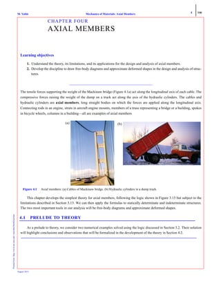
  • 1. 4 146 Mechanics of Materials: Axial MembersM. VablePrintedfrom:http://www.me.mtu.edu/~mavable/MoM2nd.htm August 2012 CHAPTER FOUR AXIAL MEMBERS Learning objectives 1. Understand the theory, its limitations, and its applications for the design and analysis of axial members. 2. Develop the discipline to draw free-body diagrams and approximate deformed shapes in the design and analysis of struc- tures. _______________________________________________ The tensile forces supporting the weight of the Mackinaw bridge (Figure 4.1a) act along the longitudinal axis of each cable. The compressive forces raising the weight of the dump on a truck act along the axis of the hydraulic cylinders. The cables and hydraulic cylinders are axial members, long straight bodies on which the forces are applied along the longitudinal axis. Connecting rods in an engine, struts in aircraft engine mounts, members of a truss representing a bridge or a building, spokes in bicycle wheels, columns in a building—all are examples of axial members This chapter develops the simplest theory for axial members, following the logic shown in Figure 3.15 but subject to the limitations described in Section 3,13. We can then apply the formulas to statically determinate and indeterminate structures. The two most important tools in our analysis will be free-body diagrams and approximate deformed shapes. 4.1 PRELUDE TO THEORY As a prelude to theory, we consider two numerical examples solved using the logic discussed in Section 3.2. Their solution will highlight conclusions and observations that will be formalized in the development of the theory in Section 4.2. Figure 4.1 Axial members: (a) Cables of Mackinaw bridge. (b) Hydraulic cylinders in a dump truck. (a) (b)
  • 2. 4 147 Mechanics of Materials: Axial MembersM. VablePrintedfrom:http://www.me.mtu.edu/~mavable/MoM2nd.htm August 2012 EXAMPLE 4.1 Two thin bars are securely attached to a rigid plate, as shown in Figure 4.2. The cross-sectional area of each bar is 20 mm2 . The force F is to be placed such that the rigid plate moves only horizontally by 0.05 mm without rotating. Determine the force F and its location h for the following two cases: (a) Both bars are made from steel with a modulus of elasticity E = 200 GPa. (b) Bar 1 is made of steel (E = 200 GPa) and bar 2 is made of aluminum (E = 70 GPa). PLAN The relative displacement of point B with respect to A is 0.05 mm, from which we can find the axial strain. By multiplying the axial strain by the modulus of elasticity, we can obtain the axial stress. By multiplying the axial stress by the cross-sectional area, we can obtain the internal axial force in each bar. We can draw the free-body diagram of the rigid plate and by equilibrium obtain the force F and its location h. SOLUTION 1. Strain calculations: The displacement of B is uB = 0.05 mm. Point A is built into the wall and hence has zero displacement. The normal strain is the same in both rods: (E1) 2. Stress calculations: From Hooke’s law σ = Eε, we can find the normal stress in each bar for the two cases. Case (a): Because E and ε1 are the same for both bars, the stress is the same in both bars. We obtain (E2) Case (b): Because E is different for the two bars, the stress is different in each bar (E3) (E4) 3. Internal forces: Assuming that the normal stress is uniform in each bar, we can find the internal normal force from N = σA, where A = 20 mm2 = 20 × 10–6 m2 . Case (a): Both bars have the same internal force since stress and cross-sectional area are the same, (E5) Case (b): The equivalent internal force is different for each bar as stresses are different. (E6) (E7) 4. External force: We make an imaginary cut through the bars, show the internal axial forces as tensile, and obtain free-body diagram shown in Figure 4.3. By equilibrium of forces in x direction we obtain (E8) By equilibrium of moment point O in Figure 4.3, we obtain (E9) (E10) Case (a): Substituting Equation (E5) into Equations (E8) and (E10), we obtain F and h: ANS. F = 2000 N h = 10 mm Case (b): Substituting Equations (E6) and (E7) into Equations (E8) and (E10), we obtain F and h: 200 mm Bar 1 Bar 2 A x B F h 20 mm Figure 4.2 Axial bars in Example 4.1. ε1 ε2 uB uA– xB xA– ------------------ 0.05 mm 200 mm --------------------- 250 μmm/mm= = = = σ1 σ2 200 10 9 × N/m 2 ( ) 250× 10 6– × 50 10 6 × N/m 2 (T)= = = σ1 E1ε1 200 10 9 × N/m 2 ( ) 250× 10 6– × 50 10 6 × N/m 2 (T)= = = σ2 E2ε2 70 10 9 × 250 10 6– ×× 17.5 10 6 × N/m 2 (T)= = = N1 N2 50 10 6 × N/m 2 ( ) 20 10 6– × m 2 ( ) 1000 N (T)= = = N1 σ1A1 50 10× 6 N/m 2 ( ) 20 10 6– × m 2 ( ) 1000 N (T)= = = N2 σ2A2 17.5 10× 6 N/m 2 ( ) 20 10 6– × m 2 ( ) 350 N (T)= = = F N1 N2+= N1 20 h–( ) N2h– 0= h 20N1 N1 N2+ --------------------= FN1 N2NN O h 20 mm Figure 4.3 Free-body diagram in Example 4.1. F 1000 N 1000 N+ 2000 N= = h 20 mm 1000 N× 1000 N 1000 N+( ) ----------------------------------------------- 10 mm= =
  • 3. 4 148 Mechanics of Materials: Axial MembersM. VablePrintedfrom:http://www.me.mtu.edu/~mavable/MoM2nd.htm August 2012 ANS. F = 1350 N h = 14.81 mm COMMENTS 1. Both bars, irrespective of the material, were subjected to the same axial strain. This is the fundamental kinematic assumption in the development of the theory for axial members, discussed in Section 4.2. 2. The sum on the right in Equation (E8) can be written where σi is the normal stress in the ith bar, ΔAi is the cross-sec- tional area of the ith bar, and n = 2 reflects that we have two bars in this problem. If we had n bars attached to the rigid plate, then the total axial force would be given by summation over n bars. As we increase the number of bars n to infinity, the cross-sectional area ΔAi tends to zero (or infinitesimal area dA) as we try to fit an infinite number of bars on the same plate, resulting in a continuous body. The sum then becomes an integral, as discussed in Section 4.1.1. 3. If the external force were located at any point other than that given by the value of h, then the plate would rotate. Thus, for pure axial problems with no bending, a point on the cross section must be found such that the internal moment from the axial stress distribution is zero. To emphasize this, consider the left side of Equation (E9), which can be written as where yi is the coordinate of the ith rod’s centroid. The summation is an expression of the internal moment that is needed for static equivalency. This internal moment must equal zero if the problem is of pure axial deformation, as discussed in Section 4.1.1. 4. Even though the strains in both bars were the same in both cases, the stresses were different when E changed. Case (a) corresponds to a homogeneous cross section, whereas case (b) is analogous to a laminated bar in which the non-homogeneity affects the stress distri- bution. 4.1.1 Internal Axial Force In this section we formalize the key observation made in Example 4.1: the normal stress σxx can be replaced by an equiva- lent internal axial force using an integral over the cross-sectional area. Figure 4.4 shows the statically equivalent systems. The axial force on a differential area σxx dA can be integrated over the entire cross section to obtain (4.1) If the normal stress distribution σxx is to be replaced by only an axial force at the origin, then the internal moments My and Mz must be zero at the origin, and from Figure 4.4 we obtain (4.2a) (4.2b) Equations (4.1), (4.2a), and (4.2b) are independent of the material models because they represent static equivalency between the normal stress on the cross section and internal axial force. If we were to consider a laminated cross section or nonlin- ear material, then it would affect the value and distribution of σxx across the cross section, but Equation (4.1) relating σxx and N would remain unchanged, and so would the zero moment condition of Equations (4.2a) and (4.2b). Equations (4.2a) and (4.2b) are used to determine the location at which the internal and external forces have to act for pure axial problem without bending, as dis- cussed in Section 4.2.6. F 1000 N 350 N+ 1350 N= = h 20 mm 1000 N× 1000 N 350 N+( ) -------------------------------------------- 14.81 mm= = σi ΔAi, i=1 n=2 ∑ yiσi ΔAi, i=1 n ∑ N σxx Ad A ∫= x y y dNdd ϭ ␴xx␴ dAx O z Figure 4.4 Statically equivalent internal axial force. O x y N yσxx Ad A ∫ 0= zσxx dA 0= A ∫
  • 4. 4 149 Mechanics of Materials: Axial MembersM. VablePrintedfrom:http://www.me.mtu.edu/~mavable/MoM2nd.htm August 2012 EXAMPLE 4.2 Figure 4.5 shows a homogeneous wooden cross section and a cross section in which the wood is reinforced with steel. The normal strain for both cross sections is uniform, εxx = −200 μ. The moduli of elasticity for steel and wood are Esteel = 30,000 ksi and Ewood = 8000 ksi. (a) Plot the σxx distribution for each of the two cross sections shown. (b) Calculate the equivalent internal axial force N for each cross section using Equation (4.1). PLAN (a) Using Hooke’s law we can find the stress values in each material. Noting that the stress is uniform in each material, we can plot it across the cross section. (b) For the homogeneous cross section we can perform the integration in Equation (4.1) directly. For the nonhomo- geneous cross section we can write the integral in Equation (4.1) as the sum of the integrals over steel and wood and then perform the integra- tion to find N. SOLUTION (a) From Hooke’s law we can write (E1) (E2) For the homogeneous cross section the stress distribution is as given in Equation (E1), but for the laminated case it switches to Equation (E2), depending on the location of the point where the stress is being evaluated, as shown in Figure 4.6. (b) Homogeneous cross section: Substituting the stress distribution for the homogeneous cross section in Equation (4.1) and integrat- ing, we obtain the equivalent internal axial force, (E3) ANS. N = 4.8 kips (C) Laminated cross section: The stress value changes as we move across the cross section. Let Asb and Ast represent the cross-sectional areas of steel at the bottom and the top. Let Aw represent the cross-sectional area of wood. We can write the integral in Equation (4.1) as the sum of three integrals, substitute the stress values of Equations (E1) and (E2), and perform the integration: or (E4) or (E5) (E6) ANS. N = 9.2 kips (C) Figure 4.5 Cross sections in Example 4.2. (a) Homogeneous. (b) Laminated. y z 2 in. 1 1 2 --- in.Wood Steel Wood 2 in. Wood Steel Steel y z 1 in. 1/4 in. 1/4 in. (a) (b) σxx( )wood 8000 ksi( ) 200–( )10 6– 1.6 ksi–= = σxx( )steel 30000 ksi( ) 200–( )10 6– 6 ksi–= = (a) 6 ksi (b) 6 ksi 1.6 ksi Figure 4.6 Stress distributions in Example 4.2. (a) Homogeneous cross section. (b) Laminated cross section. N σxx( )wood Ad A ∫ σxx( )wood A 1.6 ksi–( ) 2 in.( ) 1.5 in.( ) 4.8– kips= = = = N σxx A σxx A σxx Ad Ast ∫+d Aw ∫+d Asb ∫ σxx( )steel A σxx( )wood A σxx( )steel Ad Ast ∫+d Aw ∫+d Asb ∫= = N σxx( )steel Asb σxx( )wood Aw σxx( )steel Ast+ += N 6 ksi–( ) 2 in.( ) 1 4 --- in. ⎝ ⎠ ⎛ ⎞ 1.6 ksi–( ) 1 in.( ) 2 in.( ) 6 ksi–( ) 2 in.( ) 1 4 --- in. ⎝ ⎠ ⎛ ⎞+ + 9.2– kips= =
  • 5. 4 150 Mechanics of Materials: Axial MembersM. VablePrintedfrom:http://www.me.mtu.edu/~mavable/MoM2nd.htm August 2012 COMMENTS 1. Writing the integral in the internal axial force as the sum of integrals over each material, as in Equation (E4), is equivalent to calculat- ing the internal force carried by each material and then summing, as shown in Figure 4.7. 2. The cross section is geometrically as well as materially symmetric. Thus we can locate the origin on the line of symmetry. If the lower steel strip is not present, then we will have to determine the location of the equivalent force. 3. The example demonstrates that although the strain is uniform across the cross section, the stress is not. We considered material non- homogeneity in this example. In a similar manner we can consider other models, such as elastic–perfectly plastic or material models that have nonlinear stress–strain curves. PROBLEM SET 4.1 4.1 Aluminum bars (E = 30,000 ksi) are welded to rigid plates, as shown in Figure P4.1. All bars have a cross-sectional area of 0.5 in2 . Due to the applied forces the rigid plates at A, B, C, and D are displaced in x direction without rotating by the following amounts: uA = −0.0100 in., uB = 0.0080 in., uC = −0.0045 in., and uD = 0.0075 in. Determine the applied forces F1, F2, F3, and F4. 4.2 Brass bars between sections A and B, aluminum bars between sections B and C, and steel bars between sections C and D are welded to rigid plates, as shown in Figure P4.2. The rigid plates are displaced in the x direction without rotating by the following amounts: uB = −1.8 mm, uC = 0.7 mm, and uD = 3.7 mm. Determine the external forces F1, F2, and F3 using the properties given in Table P4.2 4.3 The ends of four circular steel bars (E = 200 GPa) are welded to a rigid plate, as shown in Figure P4.3. The other ends of the bars are built into walls. Owing to the action of the external force F, the rigid plate moves to the right by 0.1 mm without rotating. If the bars have a diameter of 10 mm, determine the applied force F. 4.4 Rigid plates are securely fastened to bars A and B, as shown in Figure P4.4. A gap of 0.02 in. exists between the rigid plates before the forces are applied. After application of the forces the normal strain in bar A was found to be 500 μ. The cross-sectional area and the modulus of Figure 4.7 Statically equivalent internal force in Example 4.2 for laminated cross section. 6 ksi 6 ksi F1 F4F x 36 in 50 in 36 in F2FF F3FF F1 F4FF2FF F3FF A B C D FigureP4.1 F1 F2FF F3FF F3FF F2FFF1 x DCBA 1.5 m 2.5 m 2 mFigure P4.2 TABLE P4.2 Brass Aluminum Steel Modulus of elasticity 70 GPa 100 GPa 200 GPa Diameter 30 mm 25 mm 20 mm 1.5 m F F 2.5 m Rigid plate Figure P4.3
  • 6. 4 151 Mechanics of Materials: Axial MembersM. VablePrintedfrom:http://www.me.mtu.edu/~mavable/MoM2nd.htm August 2012 elasticity for each bar are as follows: AA = 1 in.2 , EA = 10,000 ksi, AB = 0.5 in.2 , and EB = 30,000 ksi. Determine the applied forces F, assuming that the rigid plates do not rotate. 4.5 The strain at a cross section shown in Figure P4.5 of an axial rod is assumed to have the uniform value εxx = 200 μ. (a) Plot the stress dis- tribution across the laminated cross section. (b) Determine the equivalent internal axial force N and its location from the bottom of the cross section. Use Ealu = 100 GPa, Ewood = 10 GPa, and Esteel = 200 GPa. 4.6 A reinforced concrete bar shown in Figure P4.6 is constructed by embedding 2-in. × 2-in. square iron rods. Assuming a uniform strain εxx = −1500 μ in the cross section, (a) plot the stress distribution across the cross section; (b) determine the equivalent internal axial force N. Use Eiron = 25,000 ksi and Econc = 3000 ksi. 4.2 THEORY OF AXIAL MEMBERS In this section we will follow the procedure in Section 4.1 with variables in place of numbers to develop formulas for axial deformation and stress. The theory will be developed subject to the following limitations: 1. The length of the member is significantly greater than the greatest dimension in the cross section. 2. We are away from the regions of stress concentration. 3. The variation of external loads or changes in the cross-sectional areas is gradual, except in regions of stress concentra- tion. 4. The axial load is applied such that there is no bending. 5. The external forces are not functions of time that is, we have a static problem. (See Problems 4.37, 4.38, and 4.39 for dynamic problems.) Figure 4.8 shows an externally distributed force per unit length p(x) and external forces F1 and F2 acting at each end of an axial bar. The cross-sectional area A(x) can be of any shape and could be a function of x. Sign convention: The displacement u is considered positive in the positive x direction. The internal axial force N is considered positive in tension negative in compression. Bar A Bar B Bar A Bar B in 0.02 in F F 60 in Rigid plates Figure P4.4 Figure P4.5 80 mm 100 mm 10 mm Aluminum 10 mm Steel Wood z x y z x y 4 i 4 i 4 in 4 inFigure P4.6
  • 7. 4 152 Mechanics of Materials: Axial MembersM. VablePrintedfrom:http://www.me.mtu.edu/~mavable/MoM2nd.htm August 2012 The theory has two objectives: 1. To obtain a formula for the relative displacements u2 − u1 in terms of the internal axial force N. 2. To obtain a formula for the axial stress σxx in terms of the internal axial force N. We will take Δx = x2 − x1 as an infinitesimal distance so that the gradually varying distributed load p(x) and the cross-sec- tional area A(x) can be treated as constants. We then approximate the deformation across the cross section and apply the logic shown in Figure 4.9. The assumptions identified as we move from each step are also points at which complexities can later be added, as discussed in examples and “Stretch Yourself” problems. 4.2.1 Kinematics Figure 4.10 shows a grid on an elastic band that is pulled in the axial direction. The vertical lines remain approximately vertical, but the horizontal distance between the vertical lines changes. Thus all points on a vertical line are displaced by equal amounts. If this surface observation is also true in the interior of an axial member, then all points on a cross-section displace by equal amounts, but each cross-section can displace in the x direction by a different amount, leading to Assumption 1. Figure 4.8 Segment of an axial bar. u2 u1 x y z x1 F2FF x2 Figure 4.9 Logic in mechanics of materials. x y (a) (b) Figure 4.10 Axial deformation: (a) original grid; (b) deformed grid. (c) u is constant in y direction. (c)
  • 8. 4 153 Mechanics of Materials: Axial MembersM. VablePrintedfrom:http://www.me.mtu.edu/~mavable/MoM2nd.htm August 2012 Assumption 1 Plane sections remain plane and parallel. Assumption 1 implies that u cannot be a function of y but can be a function of x (4.3) As an alternative perspective, because the cross section is significantly smaller than the length, we can approximate a function such as u by a constant treating it as uniform over a cross section. In Chapter 6, on beam bending, we shall approximate u as a linear function of y. 4.2.2 Strain Distribution Assumption 2 Strains are small.1 If points x2 and x1 are close in Figure 4.8, then the strain at any point x can be calculated as or (4.4) Equation (4.4) emphasizes that the axial strain is uniform across the cross section and is only a function of x. In deriving Equa- tion (4.4) we made no statement regarding material behavior. In other words, Equation (4.4) does not depend on the material model if Assumptions 1 and 2 are valid. But clearly if the material or loading is such that Assumptions 1 and 2 are not tenable, then Equation (4.4) will not be valid. 4.2.3 Material Model Our motivation is to develop a simple theory for axial deformation. Thus we make assumptions regarding material behavior that will permit us to use the simplest material model given by Hooke’s law. Assumption 3 Material is isotropic. Assumption 4 Material is linearly elastic.2 Assumption 5 There are no inelastic strains.3 Substituting Equation (4.4) into Hooke’s law, that is, we obtain (4.5) Though the strain does not depend on y or z, we cannot say the same for the stress in Equation (4.5) since E could change across the cross section, as in laminated or composite bars. 4.2.4 Formulas for Axial Members Substituting σxx from Equation (4.5) into Equation (4.1) and noting that du/dx is a function of x only, whereas the integration is with respect to y and z (dA = dy dz), we obtain (4.6) 1 See Problem 4.40 for large strains. 2 See Problem 4.36 for nonlinear material behavior. 3 Inelastic strains could be due to temperature, humidity, plasticity, viscoelasticity, and so on. We shall consider inelastic strains due to tem- perature in Section 4.5. u u x( )= εxx Δx 0→ lim u2 u1– x2 x1– ----------------- ⎝ ⎠ ⎛ ⎞ Δx 0→ lim Δu Δx ------- ⎝ ⎠ ⎛ ⎞= = εxx du dx ------ x( )= σxx E εxx,= σxx E du dx ------= N E du dx ------ Ad A ∫ du dx ------ E dA A ∫= =
  • 9. 4 154 Mechanics of Materials: Axial MembersM. VablePrintedfrom:http://www.me.mtu.edu/~mavable/MoM2nd.htm August 2012 Consistent with the motivation for the simplest possible formulas, E should not change across the cross section as implied in Assumption 6. We can take E outside the integral. Assumption 6 Material is homogeneous across the cross section. With material homogeneity, we then obtain or (4.7) The higher the value of EA, the smaller will be the deformation for a given value of the internal force. Thus the rigidity of the bar increases with the increase in EA. This implies that an axial bar can be made more rigid by either choosing a stiffer mate- rial (a higher value of E) or increasing the cross-sectional area, or both. Example 4.5 brings out the importance of axial rigidity in design. The quantity EA is called axial rigidity. Substituting Equation (4.7) into Equation (4.5), we obtain (4.8) In Equation (4.8), N and A do not change across the cross section and hence axial stress is uniform across the cross section. We have used Equation (4.8) in Chapters 1 and 3, but this equation is valid only if all the limitations are imposed, and if Assump- tions 1 through 6 are valid. We can integrate Equation (4.7) to obtain the deformation between two points: (4.9) where u1 and u2 are the displacements of sections at x1 and x2, respectively. To obtain a simple formula we would like to take the three quantities N, E, and A outside the integral, which means these quantities should not change with x. To achieve this simplicity, we make the following assumptions: Assumption 7 The material is homogeneous between x1 and x2. (E is constant) Assumption 8 The bar is not tapered between x1 and x2. (A is constant) Assumption 9 The external (hence internal) axial force does not change with x between x1 and x2. (N is constant) If Assumptions 7 through 9 are valid, then N, E, and A are constant between x1 and x2, and we obtain (4.10) In Equation (4.10), points x1 and x2 must be chosen such that neither N, E, nor A changes between these points. 4.2.5 Sign Convention for Internal Axial Force The axial stress σxx was replaced by a statically equivalent internal axial force N. Figure 4.11 shows the sign convention for the positive axial force as tension. N is an internal axial force that has to be determined by making an imaginary cut and drawing a free-body diagram. In what direction should N be drawn on the free-body diagram? There are two possibilities: 1. N is always drawn in tension on the imaginary cut as per our sign convention. The equilibrium equation then gives a positive or a negative value for N. A positive value of σxx obtained from Equation (4.8) is tensile and a negative value is N E xd du Ad A ∫ EA xd du = = xd du N EA -------= σxx N A ----= u2 u1– ud u1 u2 ∫ N EA ------- x1 x2 ∫ dx= = u2 u1– N x2 x1–( ) EA --------------------------= ϩNFigure 4.11 Sign convention for positive internal axial force.
  • 10. 4 155 Mechanics of Materials: Axial MembersM. VablePrintedfrom:http://www.me.mtu.edu/~mavable/MoM2nd.htm August 2012 compressive. Similarly, the relative deformation obtained from Equation (4.10) is extension for positive values and con- traction for negative values. The displacement u will be positive in the positive x direction. 2. N is drawn on the imaginary cut in a direction to equilibrate the external forces. Since inspection is being used in determining the direction of N, tensile and compressive σxx and extension or contraction for the relative deformation must also be determined by inspection. 4.2.6 Location of Axial Force on the Cross Section For pure axial deformation the internal bending moments must be zero. Equations (4.2a) and (4.2b) can then be used to deter- mine the location of the point where the internal axial force and hence the external forces must pass for pure axial problems. Substituting Equation (4.5) into Equations (4.2a) and (4.2b) and noting that du/dx is a function of x only, whereas the integration is with respect to y and z (dA = dy dz), we obtain or (4.11a) or (4.11b) Equations (4.11a) and (4.11b) can be used to determine the location of internal axial force for composite materials. If the cross section is homogenous (Assumption 6), then E is constant across the cross section and can be taken out side the integral: (4.12a) (4.12b) Equations (4.12a) and (4.12b) are satisfied if y and z are measured from the centroid. (See Appendix A.4.) We will have pure axial deformation if the external and internal forces are colinear and passing through the centroid of a homogenous cross sec- tion. This assumes implicitly that the centroids of all cross sections must lie on a straight line. This eliminates curved but not tapered bars. 4.2.7 Axial Stresses and Strains In the Cartesian coordinate system all stress components except σxx are assumed zero. From the generalized Hooke’s law for iso- tropic materials, given by Equations (3.14a) through (3.14c), we obtain the normal strains for axial members: (4.13) where ν is the Poisson’s ratio. In Equation (4.13), the normal strains in y and z directions are due to Poisson’s effect. Assumption 1, that plane sections remain plane and parallel implies that no right angle would change during deformation, and hence the assumed deformation implies that shear strains in axial members are zero. Alternatively, if shear stresses are zero, then by Hooke’s law shear strains are zero. yσxx Ad A ∫ yE du dx ------ Ad A ∫ du dx ------ yE Ad A ∫ 0= = = yE Ad A ∫ 0= zσxx dA zE du dx ------ Ad A ∫= A ∫ du dx ------ zE Ad A ∫ 0= = zE Ad A ∫ 0= y Ad A ∫ 0= z Ad A ∫ 0= εxx σxx E -------- εyy νσxx E -----------–= νεxx εzz νσxx E -----------–=– νεxx–= = =
  • 11. 4 156 Mechanics of Materials: Axial MembersM. VablePrintedfrom:http://www.me.mtu.edu/~mavable/MoM2nd.htm August 2012 EXAMPLE 4.3 Solid circular bars of brass (Ebr = 100 GPa, νbr = 0.34) and aluminum (Eal = 70 GPa, νal = 0.33) having 200 mm diameter are attached to a steel tube (Est = 210 GPa, νst = 0.3) of the same outer diameter, as shown in Figure 4.12. For the loading shown determine: (a) The movement of the plate at C with respect to the plate at A. (b) The change in diameter of the brass cylinder. (c) The maximum inner diam- eter to the nearest millimeter in the steel tube if the factor of safety with respect to failure due to yielding is to be at least 1.2. The yield stress for steel is 250 MPa in tension. PLAN (a) We make imaginary cuts in each segment and determine the internal axial forces by equilibrium. Using Equation (4.10) we can find the relative movements of the cross sections at B with respect to A and at C with respect to B and add these two relative displacements to obtain the relative movement of the cross section at C with respect to the section at A. (b) The normal stress σxx in AB can be obtained from Equation (4.8) and the strain εyy found using Equation (4.13). Multiplying the strain by the diameter we obtain the change in diam- eter. (c) We can calculate the allowable axial stress in steel from the given failure values and factor of safety. Knowing the internal force in CD we can find the cross-sectional area from which we can calculate the internal diameter. SOLUTION (a) The cross-sectional areas of segment AB and BC are (E1) We make imaginary cuts in segments AB, BC, and CD and draw the free-body diagrams as shown in Figure 4.13. By equilibrium of forces we obtain the internal axial forces (E2) We can find the relative movement of point B with respect to point A, and C with respect to B using Equation (4.10): (E3) (E4) Adding Equations (E3) and (E4) we obtain the relative movement of point C with respect to A: (E5) ANS. uC − uA = 0.7845 mm contraction (b) We can find the axial stress σxx in AB using Equation (4.8): (E6) Substituting σxx, Ebr = 100 GPa, νbr = 0.34 in Equation (4.13), we can find εyy. Multiplying εyy by the diameter of 200 mm, we then obtain the change in diameter Δd, (E7) ANS. Δd = −0.032 mm (c) The axial stress in segment CD is Figure 4.12 Axial member in Example 4.3. 2000 kN 2000 kN 2750 kN 2750 kN 1500 kN 1500 kN 750 kN 750 kN A x 0.5 m 1.5 m 0.6 m AAB ABC π 4 --- 0.2 m( ) 2 31.41 10× 3– m 2 = = = NAB 1500 kN= NBC 1500 kN 3000 kN– 1500 kN–= = NCD 4000 kN= = 750 kN 750 kN NABN Figure 4.13 Free body diagrams in Example 4.3. NBCN 750 kN 750 kN 1500 kN 1500 kN NCD 2000 kN 2000 kN (a) (b) (c) uB uA NAB xB xA–( ) EABAAB ---------------------------------=– 1500 10 3 × N( ) 0.5 m( ) 100 10 9 × N/m 2 ( ) 31.41 10× 3– m 2 ( ) ----------------------------------------------------------------------------------------- 0.2388 10 3– × m= = uC uB– NBC xC xB–( ) EBCABC --------------------------------- 1500– 10× 3 N( ) 1.5 m( ) 70 10× 9 N/m 2 ( ) 31.41 10× 3– m 2 ( ) -------------------------------------------------------------------------------------- 1.0233 10 3– ×– m= = = uC uA– uC uB–( ) uB uA–( )+ 0.2388 m 1.0233 m–( )10 3– 0.7845 10 3– × m–= = = σxx NAB AAB ---------- 1500 10× 3 N 31.41 10× 3– m 2 ( ) --------------------------------------------- 47.8 10× 6 N/m 2 = = = εyy νbrσxx Ebr ---------------– 0.34 47.8 10× 6 N/m 2 ( ) 100 10× 9 N/m 2 --------------------------------------------------------– 0.162 10× 3– –= = Δd 200 mm --------------------= =
  • 12. 4 157 Mechanics of Materials: Axial MembersM. VablePrintedfrom:http://www.me.mtu.edu/~mavable/MoM2nd.htm August 2012 (E8) Using the given factor of safety, we determine the value of Di: or (E9) To the nearest millimeter, the diameter that satisfies the inequality in Equation (E9) is 124 mm. ANS. Di = 124 mm COMMENTS 1. On a free-body diagram some may prefer to show N in a direction that counterbalances the external forces, as shown in Figure 4.14. In such cases the sign convention is not being followed. We note that uB− uA = 0.2388 (10−3 ) m is extension and uC − uB = 1.0233 (10−3 ) m is contraction. To calculate uC − uA we must now manu- ally subtract uC − uB from uB− uA . 2. An alternative way of calculating of uC − uA is or, written more compactly, (4.14) where n is the number of segments on which the summation is performed, which in our case is 2. Equation (4.14) can be used only if the sign convention for the internal force N is followed. 3. Note that NBC − NAB = −3000 kN and the magnitude of the applied external force at the section at B is 3000 kN. Similarly, NCD − NBC = 5500 kN, which is the magnitude of the applied external force at the section at C. In other words, the internal axial force jumps by the value of the external force as one crosses the external force from left to right. We will make use of this observation in the next sec- tion, when we develop a graphical technique for finding the internal axial force. 4.2.8 Axial Force Diagram In Example 4.3 we constructed several free-body diagrams to determine the internal axial force in different segments of the axial member. An axial force diagram is a graphical technique for determining internal axial forces, which avoids the repetition of drawing free-body diagrams. An axial force diagram is a plot of the internal axial force N versus x. To construct an axial force diagram we create a small template to guide us in which direction the internal axial force will jump, as shown in Figure 4.15a and Figure 4.15b. An axial template is a free-body diagram of a small segment of an axial bar created by making an imaginary cut just before and just after the section where the external force is applied. σCD NCD ACD ----------- 4000 10 3 × N π 4⁄( ) 0.2 m( ) 2 Di 2 –[ ] ------------------------------------------------------ 16,000 10 3 × π 0.2 2 Di 2 –( )[ ] ------------------------------------ N/m 2 = = = K σyield σCD ------------- 250 10 6 π 0.2 2 Di 2 –( )[ ]×× 16,000 10 3 × ------------------------------------------------------------------ 49.09 0.2 2 Di 2 –( ) 1.2≥= = = Di 2 0.2 2 24.45 10 3– ×–≤ or Di 124.7 10 3– × m≤ NBCN 1500 kN 1500 kN 750 kN 750 kN (b) NABN 750 kN 750 kN (a) Figure 4.14 Alternative free body diagrams in Example 4.3. uC uA– N EA ------- dx xA xC ∫ NAB EABAAB -------------------- dx NBC EBCABC -------------------- dx xB xC ∫+ xA xB ∫= = uC uB– ⎫ ⎬ ⎭ uB uA–⎫ ⎬ ⎭ Δu Ni Δxi EiAi --------------- i 1= n ∑= N1 N2NN FextFF 2 FextF 2 Figure 4.15 Axial bar templates. N2 = N1 − Fext (a) N1 N2NN FextF 2 FextFF 2 N2 = N1 + Fextt (b) Template Equations
  • 13. 4 158 Mechanics of Materials: Axial MembersM. VablePrintedfrom:http://www.me.mtu.edu/~mavable/MoM2nd.htm August 2012 The external force Fext on the template can be drawn either to the left or to the right. The ends represent the imaginary cut just to the left and just to the right of the applied external force. On these cuts the internal axial forces are drawn in tension. An equilibrium equation—that is, the template equation—is written as shown in Figure 4.15 If the external force on the axial bar is in the direction of the assumed external force on the template, then the value of N2 is calculated according to the template equa- tion. If the external force on the axial bar is opposite to the direction shown on the template, then N2 is calculated by changing the sign of Fext in the template equation. Example 4.4 demonstrates the use of templates in constructing axial force diagrams. EXAMPLE 4.4 Draw the axial force diagram for the axial member shown in Example 4.3 and calculate the movement of the section at C with respect to the section at A. PLAN We can start the process by considering an imaginary extension on the left. In the imaginary extension the internal axial force is zero. Using the template in Figure 4.15a to guide us, we can draw the axial force diagram. Using Equation (4.14), we can find the relative dis- placement of the section at C with respect to the section at A. SOLUTION Let LA be an imaginary extension on the left of the shaft, as shown in Figure 4.16a. Clearly the internal axial force in the imaginary segment LA is zero. As one crosses the section at A, the internal force must jump by the applied axial force of 1500 kN. Because the forces at A are in the opposite direction to the force Fext shown on the template in Figure 4.15a, we must use opposite signs in the template equation. The internal force just after the section at A will be +1500 kN. This is the starting value in the internal axial force diagram. We approach the section at B with an internal force value of +1500 kN. The force at B is in the same direction as the force shown on the template in Figure 4.15a. Hence we subtract 3000 as per the template equation, to obtain a value of −1500 kN, as shown in Figure 4.16b. We now approach the section at C with an internal force value of −1500 kN and note that the forces at C are opposite to those on the tem- plate in Figure 4.15a. Hence we add 5500 to obtain +4000 kN. The force at D is in the same direction as that on the template in Figure 4.15a, and after subtracting we obtain a zero value in the imagi- nary extended bar DR. The return to zero value must always occur because the bar is in equilibrium. From Figure 4.16b the internal axial forces in segments AB and BC are NAB = 1500 kN and NBC = −1500 kN. The crosssectional areas as calcu- lated in Example 4.3 are and modulas of elasticity for the two sections are EAB = 100 GPa and EBC= 70 GPa. Substituting these values into Equation (4.14) we obtain the relative deformation of the section at C with respect to the section at A, (E1) or (E2) ANS. uC − uA = 0.7845 mm contraction COMMENT 1. We could have used the template in Figure 4.15b to create the axial force diagram.We approach the section at A and note that the +1500 kN is in the same direction as that shown on the template of Figure 4.15b. As per the template equation we add. Thus our starting value is +1500 kN, as shown in Figure 4.16. As we approach the section at B, the internal force N1 is +1500 kN, and the applied force of 3000 kN is in the opposite direction to the template of Figure 4.15b, so we subtract to obtain N2 as –1500 kN. We approach the section at C and note that the applied force is in the same direction as the applied force on the template of Figure 4.15b. Hence we add 5500 kN to obtain +4000 kN. The force at section D is opposite to that shown on the template of Figure 4.15b, so we subtract 4000 to get a zero value in the extended portion DR. The example shows that the direction of the external force Fext on the template is immaterial. 2000 kN 2000 kN 2750 kN 2750 kN 1500 kN 1500 kN 750 kN 750 kN A L R 0.5 m 1.5 m 0.6 m Figure 4.16 (a) Extending the axial bar for an axial force diagram. (b) Axial force diagram. N (kN)N A B C D 4000 1500 Ϫ1500 x (a) (b) AAB ABC 31.41 10× 3– m 2 = = Δu uC uA– NAB xB xA–( ) EABAAB --------------------------------- NBC xC xB–( ) EBCABC ---------------------------------+= = uC uA– 1500 10× 3 N( ) 0.5 m( ) 100 10× 9 N/m 2 ( ) 31.41 10× 3– m 2 ( ) ----------------------------------------------------------------------------------------- 1500– 10× 3 N( ) 1.5 m( ) 70 109× N/m 2 ( ) 31.41 10× 3– m 2 ( ) --------------------------------------------------------------------------------------+ 0.7845 10 3– × m–= =
  • 14. 4 159 Mechanics of Materials: Axial MembersM. VablePrintedfrom:http://www.me.mtu.edu/~mavable/MoM2nd.htm August 2012 EXAMPLE 4.5 A 1-m-long hollow rod is to transmit an axial force of 60 kN. Figure 4.17 shows that the inner diameter of the rod must be 15 mm to fit existing attachments. The elongation of the rod is limited to 2.0 mm. The shaft can be made of titanium alloy or aluminum. The modulus of elasticity E, the allowable normal stress σallow, and the density γ for the two materials is given in Table 4.1. Determine the minimum outer diameter to the nearest millimeter of the lightest rod that can be used for transmitting the axial force. PLAN The change in radius affects only the cross-sectional area A and no other quantity in Equations (4.8) and (4.10). For each material we can find the minimum cross-sectional area A needed to satisfy the stiffness and strength requirements. Knowing the minimum A for each material, we can find the minimum outer radius. We can then find the volume and hence the mass of each material and make our decision on the lighter bar. SOLUTION We note that for both materials x2 – x1 = 1 m. From Equations (4.8) and (4.10) we obtain for titanium alloy the following limits on ATi: (E1) (E2) Using similar calculations for the aluminum shaft, we obtain the following limits on AAl: (E3) (E4) Thus if , it will meet both conditions in Equations (E1) and (E2). Similarly if , it will meet both conditions in Equations (E3) and (E4). The external diameters DTi and DAl are then (E5) (E6) Rounding upward to the closest millimeter, we obtain (E7) We can find the mass of each material by taking the product of the material density and the volume of a hollow cylinder, (E8) (E9) From Equations (E8) and (E9) we see that the titanium alloy shaft is lighter. ANS. A titanium alloy shaft with an outside diameter of 25 mm should be used. COMMENTS 1. For both materials the stiffness limitation dictated the calculation of the external diameter, as can be seen from Equations (E1) and (E3). 1 m 15 mm Figure 4.17 Cylindrical rod in Example 4.5. TABLE 4.1 Material properties in Example 4.4 Material E (GPa) σallow (MPa) γ (mg/m3 ) Titanium alloy 96 400 4.4 Aluminum 70 200 2.8 Δu( )Ti 60 10× 3 N( ) 1 m( ) 96 10× 9 N/m 2 ( )ATi ------------------------------------------------- 2 10 3– m×≤= or ATi 0.313 10× 3– m 2 ≥ σmax( )Ti 60 10× 3 N( ) ATi ------------------------------- 400 10× 6 N/m 2 ≤= or ATi 0.150 10× 3– m 2 ≥ Δu( )Al 60 10× 3 N( ) 1× 28 10× 9 N/m 2 ( )AAl ------------------------------------------------- 2 10× 3– m≤= or AAl 1.071 10× 3– m 2 ≥ σmax( )Al 60 10× 3 N( ) AAl ------------------------------- 200 10× 6 N/m 2 ≤= or AAl 0.300 10× 3– m 2 ≥ ATi 0.313 10× 3– m 2 ≥ AAl 1.071 10 3– × m 2 ≥ ATi π 4 --- DTi 2 0.015 2 –( ) 0.313 10× 3– ≥= DTi 24.97 10× 3– m≤ AAl π 4 --- DAl 2 0.015 2 –( ) 1.071 10× 3– ≥= DAl 39.86 10 3– × m≤ DTi 25 10 3– ( ) m= DAl 40 10 3– ( ) m= mTi 4.4 10× 6 g/m 3 ( ) π 4 --- 0.025 2 0.015 2 –( ) m 2 ⎩ ⎭ ⎨ ⎬ ⎧ ⎫ 1 m( ) 1382 g= = mAl 2.8 10 6 × g/m 3 ( ) π 4 --- 0.040 2 0.015 2 –( ) m 2 ⎩ ⎭ ⎨ ⎬ ⎧ ⎫ 1 m( ) 3024 g= =
  • 15. 4 160 Mechanics of Materials: Axial MembersM. VablePrintedfrom:http://www.me.mtu.edu/~mavable/MoM2nd.htm August 2012 2. Even though the density of aluminum is lower than that of titanium alloy, the mass of titanium is less. Because of the higher modulus of elasticity of titanium alloy, we can meet the stiffness requirement using less material than with aluminum. 3. The answer may change if cost is a consideration. The cost of titanium per kilogram is significantly higher than that of aluminum. Thus based on material cost we may choose aluminum. However, if the weight affects the running cost, then economic analysis is needed to determine whether the material cost or the running cost is higher. 4. If in Equation (E5) we had 24.05 × 10⁻³ m on the right-hand side, our answer for DTi would still be 25 mm because we have to round upward to ensure meeting the greater-than sign requirement in Equation (E5). EXAMPLE 4.6 A rectangular aluminum bar (Eal = 10,000 ksi, ν = 0.25) of -in. thickness consists of a uniform and tapered cross section, as shown in Figure 4.18. The depth in the tapered section varies as h(x) = (2 − 0.02x) in. Determine: (a) The elongation of the bar under the applied loads. (b) The change in dimension in the y direction in section BC. PLAN (a) We can use Equation (4.10) to find uC − uB. Noting that cross-sectional area is changing with x in segment AB, we integrate Equation (4.7) to obtain uB − uA. We add the two relative displacements to obtain uC − uA and noting that uA = 0 we obtain the extension as uC. (b) Once the axial stress in BC is found, the normal strain in the y direction can be found using Equation (4.13). Multiplying by 2 in., the original length in the y direction, we then find the change in depth. SOLUTION The cross-sectional areas of AB and BC are (E1) (a) We can make an imaginary cuts in segment AB and BC, to obtain the free-body diagrams in Figure 4.19. By force equilibrium we obtain the internal forces, (E2) The relative movement of point C with respect to point B is (E3) Equation (4.7) for segment AB can be written as (E4) Integrating Equation (E4), we obtain the relative displacement of B with respect to A: or (E5) We obtain the relative displacement of C with respect to A by adding Equations (E3) and (E5): (E6) We note that point A is fixed to the wall, and thus uA = 0. ANS. uC = 0.036 in. elongation (b) The axial stress in BC is σAB = NBC /ABC = 10/1.5 = 6.667 ksi. From Equation (4.13) the normal strain in y direction can be found, 3 4 --- y P 50 in 20 in 3 4 in 4 in Figure 4.18 Axial member in Example 4.6. ABC 3 4 --- in. ⎝ ⎠ ⎛ ⎞ 2 in.( ) 1.5 in. 2 = = AAB 3 4 --- in. ⎝ ⎠ ⎛ ⎞ 2h in.( ) 1.5 2 0.02x–( ) in. 2 = = 10 kipsNBCN Figure 4.19 Free-body diagrams in Example 4.6. 10 kipsNABN NAB 10 kips= NBC 10 kips= uC uB– NBC xC xB–( ) EBCABC --------------------------------- 10 kips( ) 20 in.( ) 10,000 ksi( ) 1.5 in. 2 ( ) ------------------------------------------------------ 13.33 10 3– × in.= = = xd du ⎝ ⎠ ⎛ ⎞ AB NAB EABAAB -------------------- 10 kips 10,000 ksi( ) 1.5 2 0.02x–( ) in. 2 [ ] ---------------------------------------------------------------------------------= = du uA uB ∫ 10 3– 1.5 2 0.02x–( ) ----------------------------------- dx xA=0 xB=50 ∫ in.= uB uA– 10 3– 1.5 ----------- 1 0.02–( ) ------------------ 2 0.02x–( )ln 0 50 10 3– 0.03 ----------- 1( ) 2( )ln–ln[ ] in.– 23.1 10× 3– in.= = = uC uA– 13.33 10 3– × 23.1 10× 3– + 36.43 10 3– × in.= =
  • 16. 4 161 Mechanics of Materials: Axial MembersM. VablePrintedfrom:http://www.me.mtu.edu/~mavable/MoM2nd.htm August 2012 (E7) The change in dimension in the y direction Δv can be found as (E8) ANS. Δv = 0.3333 × 10⁻³ in. contraction COMMENT 1. An alternative approach is to integrate Equation (E4): (E9) To find constant of integration c, we note that at x = 0 the displacement u = 0. Hence, c = (10−3 /0.03) ln (2). Substituting the value, we obtain (E10) Knowing u at all x, we can obtain the extension by substituting x = 50 to get the displacement at C. EXAMPLE 4.7 The radius of a circular truncated cone in Figure 4.20 varies with x as R(x) = (r/L)(5L − 4x). Determine the extension of the truncated cone due to its own weight in terms of E, L, r, and γ, where E and γ are the modulus of elasticity and the specific weight of the material, respectively. PLAN We make an imaginary cut at location x and take the lower part of the truncated cone as the free-body diagram. In the free-body diagram we can find the volume of the truncated cone as a function of x. Multiplying the volume by the specific weight, we can obtain the weight of the truncated cone and equate it to the internal axial force, thus obtaining the internal force as a function of x. We then integrate Equa- tion (4.7) to obtain the relative displacement of B with respect to A. SOLUTION Figure 4.21 shows the free-body diagram after making a cut at some location x. We can find the volume V of the truncated cone by sub- tracting the volumes of two complete cones between C and D and between B and D. We obtain the location of point D, (E1) The volume of the truncated cone is (E2) By equilibrium of forces in Figure 4.21 we obtain the internal axial force: εyy νABσAB EΑΒ -------------------– 0.25 6.667 ksi( )× 10,000 ksi( ) --------------------------------------------– 0.1667 10× 3– –= = = Δv εyy 2 in.( ) 0.3333 10× 3– in.–= = u x( ) 10 3– 0.03 ----------- 2 0.02x–( ) c+ln–= u x( ) 10 3– 0.03 ----------- 2 0.02x– 2 ---------------------- ⎝ ⎠ ⎛ ⎞ln–= R(x) x B A r L Figure 4.20 Truncated cone in Example 4.7. D N R x) (L Ϫ x) h Figure 4.21 Free-body diagram of truncated cone in Example 4.7. R x L h+=( ) r L --- 5L 4 L h+( )–[ ] 0= = or h L 4⁄= V 1 3 ---πR2 L x– L 4 ---+ ⎝ ⎠ ⎛ ⎞ 1 3 ---πr2L 4 ---– π 12 ------ r2 L2 ----- 5L 4x–( )3 r2L–= =
  • 17. 4 162 Mechanics of Materials: Axial MembersM. VablePrintedfrom:http://www.me.mtu.edu/~mavable/MoM2nd.htm August 2012 (E3) The cross-sectional area at location x (point C) is (E4) Equation (4.7) can be written as (E5) Integrating Equation (E5) from point A to point B, we obtain the relative movement of point B with respect to point A: or (E6) Point A is built into the wall, hence uA = 0. We obtain the extension of the bar as displacement of point B. ANS. COMMENTS 1. Dimension check: We write O( ) to represent the dimension of a quantity. F has dimensions of force and L of length. Thus, the modu- lus of elasticity E, which has dimensions of force per unit area, is represented as O(F/L2 ). The dimensional consistency of our answer is then checked as 2. An alternative approach to determining the volume of the truncated cone in Figure 4.21 is to find first the volume of the infinitesimal disc shown in Figure 4.22. We then integrate from point C to point B: (E7) 3. On substituting the limits we obtain the volume given by (E2), as before: 4. The advantage of the approach in comment 2 is that it can be used for any complex function representation of R(x), such as given in Problems 4.27 and 4.28, whereas the approach used in solving the example problem is only valid for a linear representation of R(x). 4.2.9* General Approach to Distributed Axial Forces Distributed axial forces are usually due to inertial forces, gravitational forces, or frictional forces acting on the surface of the axial bar. The internal axial force N becomes a function of x when an axial bar is subjected to a distributed axial force p(x), as seen in Example 4.7. If p(x) is a simple function, then we can find N as a function of x by drawing a free-body diagram, as we did in Example 4.7. However, if the distributed force p(x) is a complex function, it may be easier to use the alternative described in this section. Consider an infinitesimal axial element created by making two imaginary cuts at a distance dx from each other, as shown in Figure 4.23. By equilibrium of forces in the x direction we obtain: or (4.15) N W γV γπr2 12L2 ------------ 5L 4x–( )3 L3–[ ]= = = A πR 2 π r2 L2 ------ 5L 4x–( )2= = xd du N EA ------- γπr2 12L2 ------------ 5L 4x–( ) 3 L 3 –[ ] Eπ r2 L2 ----- 5L 4x–( ) 2 -------------------------------------------------------= = du uA uB ∫ γ 12E ---------- 5L 4x–( ) L3 5L 4x–( ) 2 --------------------------– dx xA=0 xB=L ∫= uB uA– = γ 12E ---------- 5Lx 2x2– L3 4 5L 4x–( ) --------------------------– 0 L γL2 12E ---------- 5 2– 1 4 ---– 1 20 ------+ ⎝ ⎠ ⎛ ⎞ 7γL2 30E ------------= = uB 7γL2 30E ------------ ⎝ ⎠ ⎛ ⎞= downward γ O F L 3 ----- ⎝ ⎠ ⎛ ⎞→ L O L( )→ E O F L 2 ----- ⎝ ⎠ ⎛ ⎞→ u O L( )→ γL 2 E -------- O F L 3 ⁄( )L 2 F L 2 ⁄ ------------------------ ⎝ ⎠ ⎜ ⎟ ⎛ ⎞ O L( ) checks→→→ V Vd x L ∫ πR 2 xd x L ∫ π r 2 L 2 ----- 5L 4x–( ) 2 xd x L ∫ π r 2 L2 ----- 5L 4x–( ) 3 3 4–( ) -------------------------- x L –= = = = R(x) Figure 4.22 Alternative approach to finding volume of truncated cone. N ϩ dNddN dx Figure 4.23 Equilibrium of an axial element. N dN+( ) p x( )dx N–+ 0= dN dx ------- p x( )+ 0=
  • 18. 4 163 Mechanics of Materials: Axial MembersM. VablePrintedfrom:http://www.me.mtu.edu/~mavable/MoM2nd.htm August 2012 Equation (4.15) assumes that p(x) is positive in the positive x direction. If p(x) is zero in a segment of the axial bar, then the internal force N is a constant in that segment. Equation (4.15) can be integrated to obtain the internal force N. The integration constant can be found by knowing the value of the internal force N at either end of the bar. To obtain the value of N at the end of the shaft (say, point A), a free-body diagram is constructed after making an imaginary cut at an infinitesimal distance Δx from the end as shown in Figure 4.24) and writing the equilibrium equation as This equation shows that the distributed axial force does not affect the boundary condition on the internal axial force. The value of the internal axial force N at the end of an axial bar is equal to the concentrated external axial force applied at the end. Suppose the weight per unit volume, or, the specific weight of a bar, is γ. By multiplying the specific weight by the cross- sectional area A, we would obtain the weight per unit length. Thus p(x) is equal to γA in magnitude. If x coordinate is chosen in the direction of gravity, then p(x) is positive: [ p(x) = +γΑ]. If it is opposite to the direction of gravity, then p(x) is negative:[ p(x) = −γΑ]. EXAMPLE 4.8 Determine the internal force N in Example 4.7 using the approach outlined in Section 4.2.9. PLAN The distributed force p(x) per unit length is the product of the specific weight times the area of cross section. We can integrate Equation (4.15) and use the condition that the value of the internal force at the free end is zero to obtain the internal force as a function of x. SOLUTION The distributed force p(x) is the weight per unit length and is equal to the specific weight times the area of cross section A = πR2 = π(r2 / L2 )(5L – 4x)2 : (E1) We note that point B (x = L) is on a free surface and hence the internal force at B is zero. We integrate Equation (4.15) from L to x after substituting p(x) from Equation (E1) and obtain N as a function of x, (E2) ANS. COMMENT 1. An alternative approach is to substitute (E1) into Equation (4.15) and integrate to obtain (E3) To determine the integration constant, we use the boundary condition that at N (x = L) = 0, which yields . Substi- tuting this value into Equation (E3), we obtain N as before. FextFFNAN ␧Figure 4.24 Boundary condition on internal axial force. Δx Δx Fext NA p xA( )Δx––[ ] Δx 0→ lim 0= NA Fext= p x( ) γA γπ r 2 L 2 ----- 5L 4x–( ) 2 = = Nd NB=0 N ∫ p x( ) xd xB=L x ∫– γ π r2 L 2 ----- 5L 4x–( ) 2 xd L x ∫– γ π r2 L 2 ----- ⎝ ⎠ ⎛ ⎞– 5L 4x–( ) 3 4– 3× -------------------------- L x = = = N γπr 2 12L 2 ------------ 5L 4x–( ) 3 L 3 –[ ]= N x( ) γπr 2 12L 2 ------------ 5L 4x–( ) 3 c1+= c1 γπr2 12L2⁄( )– L 3 = Consolidate your knowledge 1. Identity five examples of axial members from your daily life. 2. With the book closed, derive Equation (4.10), listing all the assumptions as you go along.
  • 19. 4 164 Mechanics of Materials: Axial MembersM. VablePrintedfrom:http://www.me.mtu.edu/~mavable/MoM2nd.htm August 2012 PROBLEM SET 4.2 4.7 A crane is lifting a mass of 1000-kg, as shown in Figure P4.7. The weight of the iron ball at B is 25 kg. A single cable having a diameter of 25 mm runs between A and B. Two cables run between B and C, each having a diameter of 10 mm. Determine the axial stresses in the cables. 4.8 The counterweight in a lift bridge has 12 cables on the left and 12 cables on the right, as shown in Figure P4.8. Each cable has an effec- tive diameter of 0.75 in, a length of 50 ft, a modulus of elasticity of 30,000 ksi, and an ultimate strength of 60 ksi. (a) If the counterweight is 100 kips, determine the factor of safety for the cable. (b) What is the extension of each cable when the bridge is being lifted? QUICK TEST 4.1 Time: 20 minutes/Total: 20 points Answer true or false and justify each answer in one sentence. Grade yourself with the answers given in Appendix E. 1. Axial strain is uniform across a nonhomogeneous cross section. 2. Axial stress is uniform across a nonhomogeneous cross section. 3. The formula can be used for finding the stress on a cross section of a tapered axial member. 4. The formula can be used for finding the deformation of a segment of a tapered axial member. 5. The formula can be used for finding the stress on a cross section of an axial member subjected to distributed forces. 6. The formula can be used for finding the deformation of a segment of an axial member sub- jected to distributed forces. 7. The equation cannot be used for nonlinear materials. 8. The equation can be used for a nonhomogeneous cross section. 9. External axial forces must be collinear and pass through the centroid of a homogeneous cross section for no bending to occur. 10. Internal axial forces jump by the value of the concentrated external axial force at a section. σxx N A⁄= u2 u1– N x2 x1–( ) EA⁄= σxx N A⁄= u2 u1– N x2 x1–( ) EA⁄= N σxx Ad A ∫= N σxx Ad A ∫= A B CFigure P4.7
  • 20. 4 165 Mechanics of Materials: Axial MembersM. VablePrintedfrom:http://www.me.mtu.edu/~mavable/MoM2nd.htm August 2012 4.9 (a) Draw the axial force diagram for the axial member shown in Figure P4.9. (b) Check your results for part a by finding the internal forces in segments AB, BC, and CD by making imaginary cuts and drawing free-body diagrams. (c) The axial rigidity of the bar is EA = 8000 kips. Determine the movement of the section at D with respect to the section at A. 4.10 (a) Draw the axial force diagram for the axial member shown in Figure P4.10. (b) Check your results for part a by finding the internal forces in segments AB, BC, and CD by making imaginary cuts and drawing free-body diagrams. (c) The axial rigidity of the bar is EA = 80,000 kN. Determine the movement of the section at C. 4.11 (a) Draw the axial force diagram for the axial member shown in Figure P4.11. (b) Check your results for part a by finding the internal forces in segments AB, BC, and CD by making imaginary cuts and drawing free-body diagrams. (c) The axial rigidity of the bar is EA = 2000 kips. Determine the movement of the section at B. 4.12 (a) Draw the axial force diagram for the axial member shown in Figure P4.12. (b) Check your results for part a by finding the internal forces in segments AB, BC, and CD by making imaginary cuts and drawing free-body diagrams. (c) The axial rigidity of the bar is EA = 50,000 kN. Determine the movement of the section at D with respect to the section at A. Figure P4.8 Set of 12 Cables Counter-weight 25 kips 30 kips 25 kips 10 kips 20 kips 30 kips 50 in 20 in 20 in Figure P4.9 75 kN 45 kN 75 kN 70 kN 45 kN 0.5 m 0.25 m 0.25 m Figure P4.10 2 kips 4 kips 2 kips 1.5 kipsp 4 kips 60 in 25 in 20 in Figure P4.11 60 kN 90 kN 60 kN 100 kN 200 kN 90 kN 0.6 m 0.4 m 0.4 mFigure P4.12
  • 21. 4 166 Mechanics of Materials: Axial MembersM. VablePrintedfrom:http://www.me.mtu.edu/~mavable/MoM2nd.htm August 2012 4.13 Three segments of 4-in. × 2-in. rectangular wooden bars (E = 1600 ksi) are secured together with rigid plates and subjected to axial forces, as shown in Figure P4.13. Determine: (a) the movement of the rigid plate at D with respect to the plate at A; (b) the maximum axial stress. 4.14 Aluminum bars (E = 30,000 ksi) are welded to rigid plates, as shown in Figure P4.1. All bars have a cross-sectional area of 0.5 in2 . The applied forces are F1 = 8 kips, F2 = 12 kips, and F3= 9 kips. Determine (a) the displacement of the rigid plate at D with respect to the rigid plate at A. (b) the maximum axial stress in the assembly. 4.15 Brass bars between sections A and B, aluminum bars between sections B and C, and steel bars between sections C and D are welded to rigid plates, as shown in Figure P4.2. The properties of the bars are given in Table 4.2 The applied forces are F1 = 90 kN, F2 = 40 kN, and F3= 70 kN. Determine (a) the displacement of the rigid plate at D.(b) the maximum axial stress in the assembly. 4.16 A solid circular steel (Es = 30,000 ksi) rod BC is securely attached to two hollow steel rods AB and CD as shown. Determine (a) the angle of displacement of section at D with respect to section at A; (b) the maximum axial stress in the axial member. 4.17 Two circular steel bars (Es = 30,000 ksi, νs = 0.3) of 2-in. diameter are securely connected to an aluminum bar (Ea1 = 10,000 ksi, νal = 0.33) of 1.5-in. diameter, as shown in Figure P4.17. Determine (a) the displacement of the section at C with respect to the wall; (b) the maxi- mum change in the diameter of the bars. 4.18 Two cast-iron pipes (E = 100 GPa) are adhesively bonded together, as shown in Figure P4.18. The outer diameters of the two pipes are 50 mm and 70 mm and the wall thickness of each pipe is 10 mm. Determine the displacement of end B with respect to end A. Tapered axial members 4.19 The tapered bar shown in Figure P4.19 has a cross-sectional area that varies as A = K(2L − 0.25 x)2 . Determine the elongation of the bar in terms of P, L, E, and K. p p kips 50 in 30 in 30 in Figure P4.13 Figure P4.16 60 kips A B C4 in. 2 in. 24 in.36 in.24 in. D 60 kips 210 kips 100 kips 100 kips 210 kips 50 kips 50 kips 25 kips Aluminum 5 kips 17.5 kips 5 kips 17.5 kips 40 in 15 in 25 in Figure P4.17 500 mm 20 kN 150 mm A B 20 kN Figure P4.18 L Figure P4.19
  • 22. 4 167 Mechanics of Materials: Axial MembersM. VablePrintedfrom:http://www.me.mtu.edu/~mavable/MoM2nd.htm August 2012 4.20 The tapered bar shown in Figure P4.19 has a cross-sectional area that varies as . Determine the elongation of the bar in terms of P, L, E, and K. 4.21 A tapered and an untapered solid circular steel bar (E = 30,000 ksi) are securely fastened to a solid circular aluminum bar (E = 10,000 ksi), as shown in Figure P4.21. The untapered steel bar has a diameter of 2 in. The aluminum bar has a diameter of 1.5 in. The diameter of the tapered bars varies from 1.5 in to 2 in. Determine (a) the displacement of the section at C with respect to the section at A; (b) the maximum axial stress in the bar. Distributed axial force 4.22 The column shown in Figure P4.22 has a length L, modulus of elasticity E, and specific weight γ. The cross section is a circle of radius a. Determine the contraction of each column in terms of L, E, γ, and a. 4.23 The column shown in Figure P4.23 has a length L, modulus of elasticity E, and specific weight γ. The cross section is an equilateral tri- angle of side a.Determine the contraction of each column in terms of L, E, γ, and a. 4.24 The column shown in Figure P4.24 has a length L, modulus of elasticity E, and specific weight γ. The cross-sectional area is A. Deter- mine the contraction of each column in terms of L, E, γ, and A. 4.25 On the truncated cone of Example 4.7 a force P = γ πr2 L/5 is also applied, as shown in Figure P4.25. Determine the total elongation of the cone due to its weight and the applied force. (Hint: Use superposition.) A K 4L 3x–( )= 10 kips 20 kips 10 kips 60 kips40 kips 20 kips 40 in 15 in 60 in Aluminum Figure P4.21 Figure P4.22 Figure P4.23 Figure P4.24 P L 5r Figure P4.25
  • 23. 4 168 Mechanics of Materials: Axial MembersM. VablePrintedfrom:http://www.me.mtu.edu/~mavable/MoM2nd.htm August 2012 4.26 A 20-ft-tall thin, hollow tapered tube of a uniform wall thickness of is used for a light pole in a parking lot, as shown in Figure P4.26. The mean diameter at the bottom is 8 in., and at the top it is 2 in. The weight of the lights on top of the pole is 80 lb. The pole is made of aluminum alloy with a specific weight of 0.1 lb/in3 , a modulus of elasticity E = 11,000 ksi, and a shear modulus of rigidity G = 4000 ksi. Determine (a) the maximum axial stress; (b) the contraction of the pole. (Hint: Approximate the cross-sectional area of the thin-walled tube by the product of circumference and thickness.) 4.27 Determine the contraction of a column shown in Figure P4.27 due to its own weight. The specific weight is γ = 0.28 lb/in.3 , the modu- lus of elasticity is E = 3600 ksi, the length is L = 120 in., and the radius is where R and x are in inches. 4.28 Determine the contraction of a column shown in Figure P4.27 due to its own weight. The specific weight is γ= 24 kN/m3 the modulus of elasticity is E = 25 GPa, the length is L = 10 m and the radius is R = 0.5e−0.07x , where R and x are in meters. 4.29 The frictional force per unit length on a cast-iron pipe being pulled from the ground varies as a quadratic function, as shown in Figure P4.29. Determine the force F needed to pull the pipe out of the ground and the elongation of the pipe before the pipe slips, in terms of the mod- ulus of elasticity E, the cross-sectional area A, the length L, and the maximum value of the frictional force fmax. Design problems 4.30 The spare wheel in an automobile is stored under the vehicle and raised and lowered by a cable, as shown in Figure P4.30. The wheel has a mass of 25 kg. The ultimate strength of the cable is 300 MPa, and it has an effective modulus of elasticity E = 180 GPa. At maximum extension the cable length is 36 cm. (a) For a factor of safety of 4, determine to the nearest millimeter the minimum diameter of the cable if fail- ure due to rupture is to be avoided. (b) What is the maximum extension of the cable for the answer in part (a)? 1 8 --- in. Figure P4.26 Tapered pole R 240 x– ,= L Figure P4.27 x f ϭ fmaxff L2 x2 F Figure P4.29 Figure P4.30
  • 24. 4 169 Mechanics of Materials: Axial MembersM. VablePrintedfrom:http://www.me.mtu.edu/~mavable/MoM2nd.htm August 2012 4.31 An adhesively bonded joint in wood (E = 1800 ksi) is fabricated as shown in Figure P4.31. If the total elongation of the joint between A and D is to be limited to 0.05 in., determine the maximum axial force F that can be applied. 4.32 A 5-ft-long hollow rod is to transmit an axial force of 30 kips. The outer diameter of the rod must be 6 in. to fit existing attachments. The relative displacement of the two ends of the shaft is limited to 0.027 in. The axial rod can be made of steel or aluminum. The modulus of elasticity E, the allowable axial stress σallow, and the specific weight γ are given in Table 4.32. Determine the maximum inner diameter in incre- ments of of the lightest rod that can be used for transmitting the axial force and the corresponding weight. 4.33 A hitch for an automobile is to be designed for pulling a maximum load of 3600 lb. A solid square bar fits into a square tube and is held in place by a pin, as shown in Figure P4.33. The allowable axial stress in the bar is 6 ksi, the allowable shear stress in the pin is 10 ksi, and the allowable axial stress in the steel tube is 12 ksi. To the nearest in., determine the minimum cross-sectional dimensions of the pin, the bar, and the tube. (Hint: The pin is in double shear.) Stretch yourself 4.34 An axial rod has a constant axial rigidity EA and is acted upon by a distributed axial force p(x). If at the section at A the internal axial force is zero, show that the relative displacement of the section at B with respect to the displacement of the section at A is given by (4.16) 5 4.35 A composite laminated bar made from n materials is shown in Figure P4.35. Ei and Ai are the modulus of elasticity and cross sectional area of the ith material. (a) If Assumptions from 1 through 5 are valid, show that the stress in the ith material is given Equation (4.17a), where N is the total internal force at a cross section. (b) If Assumptions 7 through 9 are valid, show that relative deformation is given by Equation (4.17b). (c) Show that for E1=E2=E3....=En=E Equations (4.17a) and (4.17b) give the same results as Equations (4.8) and (4.10). TABLE P4.32 Material properties Material E (ksi) σallow (ksi) γ (lb/in.3 ) Steel 30,000 24 0.285 Aluminum 10,000 14 0.100 5 in 36 in36 inFigure P4.31 1 8 --- in. 1 16 ------ Pin Square Bar Square Tube Figure P4.33 uB uA– 1 EA ------- x xB–( )p x( ) xd xA xB ∫= σxx( )i u2 u1– 1 x y z Figure P4.35 (4.17a) (4.17b) σxx( )i NEi Ej Aj j=1 n ∑ --------------------------= u2 u1– N x2 x1–( ) Ej Aj j=1 n ∑ --------------------------=
  • 25. 4 170 Mechanics of Materials: Axial MembersM. VablePrintedfrom:http://www.me.mtu.edu/~mavable/MoM2nd.htm August 2012 4.36 The stress–strain relationship for a nonlinear material is given by the power law σ = Eεn . If all assumptions except Hooke’s law are valid, show that (4.17) and the axial stress σxx is given by (4.8). 4.37 Determine the elongation of a rotating bar in terms of the rotating speed ω, density γ, length L, modulus of elasticity E, and cross-sec- tional area A (Figure P4.37). (Hint: The body force per unit volume is ρω2 x.) 4.38 Consider the dynamic equilibrium of the differential elements shown in Figure P4.38, where N is the internal force, γ is the density, A is the cross-sectional area, and is acceleration. By substituting for N from Equation (4.7) into the dynamic equilibrium equation, derive the wave equation: (4.18) The material constant c is the velocity of propagation of sound in the material. 4.39 Show by substitution that the functions f(x − ct) and g(x + ct) satisfy the wave equation, Equation (4.18). 4.40 The strain displacement relationship for large axial strain is given by (4.19) where we recognize that as u is only a function of x, the strain from (4.19) is uniform across the cross section. For a linear, elastic, homoge- neous material show that (4.20) The axial stress σxx is given by (4.8). Computer problems 4.41 Table P4.41 gives the measured radii at several points along the axis of the solid tapered rod shown in Figure P4.41. The rod is made of aluminum (E = 100 GPa) and has a length of 1.5 m. Determine (a) the elongation of the rod using numerical integration; (b) the maximum axial stress in the rod. u2 u1– N EA ------- ⎝ ⎠ ⎛ ⎞ 1/n x2 x1–( )= L x ␻ Figure P4.37 ∂ 2 u ∂t 2 ⁄ ∂ 2 u ∂t 2 -------- c 2 ∂ 2 u ∂x 2 --------= where c E γ ---= εxx du dx ------ 1 2 --- du dx ------ ⎝ ⎠ ⎛ ⎞ 2 += du dx ------ 1 2N EA -------+ 1–= x 0 kN Figure P4.41 TABLE P4.41 x (m) R(x) (mm) x (m) R(x) (mm) 0.0 100.6 0.8 60.1 0.1 92.7 0.9 60.3 0.2 82.6 1.0 59.1 0.3 79.6 1.1 54.0 0.4 75.9 1.2 54.8 0.5 68.8 1.3 54.1 0.6 68.0 1.4 49.4 0.7 65.9 1.5 50.6
  • 26. 4 171 Mechanics of Materials: Axial MembersM. VablePrintedfrom:http://www.me.mtu.edu/~mavable/MoM2nd.htm August 2012 4.42 Let the radius of the tapered rod in Problem 4.41 be represented by the equation R(x) = a + bx. Using the data in Table P4.41 determine constants a and b by the least-squares method and then find the elongation of the rod by analytical integration. 4.43 Table 4.43 shows the values of the distributed axial force at several points along the axis of the hollow steel rod (E = 30,000 ksi) shown in Figure P4.43. The rod has a length of 36 in., an outside diameter of 1 in., and an inside diameter of 0.875 in. Determine (a) the displacement of end A using numerical integration; (b) the maximum axial stress in the rod. 4.44 Let the distributed force p(x) in Problem 4.43 be represented by the equation Using the data in Table P4.43 determine constants a, b, and c by the least-squares method and then find the displacement of the section at A by analytical integration. 4.3 STRUCTURAL ANALYSIS Structures are usually an assembly of axial bars in different orientations. Equation (4.10) assumes that the bar lies in x direction, and hence in structural analysis the form of Equation (4.21) is preferred over Equation (4.10). (4.21) where L= x2 − x1 and δ =u2 – u1 in Equation (4.10). L represents the original length of the bar and δ represents deformation of the bar in the original direction irrespective of the movement of points on the bar. It should also be recognized that L, E, and A are positive. Hence the sign of δ is the same as that of N: • If N is a tensile force, then δ is elongation. • If N is a compressive force, then δ is contraction. 4.3.1 Statically Indeterminate Structures Statically indeterminate structures arise when there are more supports than needed to hold a structure in place. These extra sup- ports are included for safety or to increase the stiffness of the structures. Each extra support introduces additional unknown reac- tions, and hence the total number of unknown reactions exceeds the number of static equilibrium equations. The degree of static redundancy is the number of unknown reactions minus the number of equilibrium equations. If the degree of static redundancy is zero, then we have a statically determinate structure and all unknowns can be found from equilibrium equations. If the degree of static redundancy is not zero, then we need additional equations to determine the unknown reactions. These additional equa- tions are the relationships between the deformations of bars. Compatibility equations are geometric relationships between the deformations of bars that are derived from the deformed shapes of the structure. The number of compatibility equations needed is always equal to the degree of static redundancy. Drawing the approximate deformed shape of a structure for obtaining compatibility equations is as important as drawing a free-body diagram for writing equilibrium equations. The deformations shown in the deformed shape of the structure must be consistent with the direction of forces drawn on the free-body diagram. Tensile (compressive) force on a bar on free body dia- gram must correspond to extension (contraction) of the bar shown in deformed shape. A x Figure P4.43 TABLE P4.43 x (inches) p(x) (lb/in.) x (in.) p(x) (lb/in.) 0 260 21 −471 3 106 24 −598 6 32 27 −645 9 40 30 −880 12 −142 33 −1035 15 −243 36 −1108 18 −262 p x( ) cx 2 bx a.+ += δ NL EA --------=
  • 27. 4 172 Mechanics of Materials: Axial MembersM. VablePrintedfrom:http://www.me.mtu.edu/~mavable/MoM2nd.htm August 2012 In many structures there are gaps between structural members. These gaps may be by design to permit expansion due to temper- ature changes, or they may be inadvertent due to improper accounting for manufacturing tolerances. We shall make use of the obser- vation that for a linear system it does not matter how we reach the final equilibrium state. We therefore shall start by assuming that at the final equilibrium state the gap is closed. At the end of analysis we will check if our assumption of gap closure is correct or incor- rect and make corrections as needed. Displacement, strain, stress, and internal force are all related as depicted by the logic shown in Figure 4.9 and incorporated in the formulas developed in Section 4.2. If one of these quantities is found, then the rest could be found for an axial member. Thus theoretically, in structural analysis, any of the four quantities could be treated as an unknown variable. Analysis however, is traditionally conducted using either forces (internal or reaction) or displacements as the unknown variables, as described in the two methods that follow. 4.3.2 Force Method, or Flexibility Method In this method internal forces or reaction forces are treated as the unknowns. The coefficient L/EA, multiplying the internal unknown force in Equation (4.21), is called the flexibility coefficient. If the unknowns are internal forces (rather than reaction forces), as is usually the case in large structures, then the matrix in the simultaneous equations is called the flexibility matrix. Reaction forces are often preferred in hand calculations because the number of unknown reactions (degree of static redundancy) is either equal to or less than the total number of unknown internal forces. 4.3.3 Displacement Method, or Stiffness Method In this method the displacements of points are treated as the unknowns. The minimum number of displacements that are neces- sary to describe the deformed geometry is called degree of freedom. The coefficient multiplying the deformation EA/L is called the stiffness coefficient. Using small-strain approximation, the relationship between the displacement of points and the defor- mation of the bars is found from the deformed shape and substituted in the compatibility equations. Using Equation (4.21) and equilibrium equations, the displacement and the external forces are related. The matrix multiplying the unknown displacements in a set of algebraic equations is called the stiffness matrix. 4.3.4 General Procedure for Indeterminate Structure The procedure outlined can be used for solving statically indeterminate structure problems by either the force method or by the displacement method. 1. If there is a gap, assume it will close at equilibrium. 2. Draw free-body diagrams, noting the tensile and compressive nature of internal forces. Write equilibrium equations relating internal forces to each other. or 3. Write equilibrium equations in which the internal forces are written in terms of reaction forces, if the force method is to be used. 4. Draw an exaggerated approximate deformed shape, ensuring that the deformation is consistent with the free body dia- grams of step 2. Write compatibility equations relating deformation of the bars to each other. or 5. Write compatibility equations in terms of unknown displacements of points on the structure, if displacement method is to be used. 6. Write internal forces in terms of deformations using Equation (4.21). 7. Solve the equations of steps 2, 3, and 4 simultaneously for the unknown forces (for force method) or for the unknown displacements (for displacement method). 8. Check whether the assumption of gap closure in step 1 is correct. Both the force method and the displacement method are used in Examples 4.10 and 4.11 to demonstrate the similarities and differences in the two methods.
  • 28. 4 173 Mechanics of Materials: Axial MembersM. VablePrintedfrom:http://www.me.mtu.edu/~mavable/MoM2nd.htm August 2012 EXAMPLE 4.9 The three bars in Figure 4.25 are made of steel (E = 30,000 ksi) and have cross-sectional areas of 1 in2 . Determine the displacement of point D PLAN The displacement of point D with respect to point C can be found using Equation (4.21). The deformation of rod AC or BC can also be found from Equation (4.21) and related to the displacement of point C using small-strain approximation. SOLUTION Figure 4.26 shows the free body diagrams. By equilibrium of forces in Figure 4.26a, we obtain (E1) By equilibrium of forces in Figure 4.26b, we obtain (E2) (E3) Substituting for θ from Figure 4.26c and solving Equations (E2) and (E3), we obtain (E4) From Equation (4.21) we obtain the relative displacement of D with respect to C as shown in Equation (E5) and deformation of bar AC in Equation (E6). (E5) (E6) Figure 4.26d shows the exaggerated deformed geometry of the two bars AC and BC. The displacement of point C can be found by (E7) Adding Equations (E5) and (E7) we obtain the displacement of point D, uD = (4.5 + 3.52)10−3 in. ANS. uD = 0.008 in COMMENT 1. This was a statically determinate problem as we could find the internal forces in all members by static equilibrium. EXAMPLE 4.10 3 in 4 in 5 in P ϭ 27 kips A C D B 3 in Figure 4.25 Geometry in Example 4.9 NCD 27 kips= NCA NCB= NCA θcos NCB θcos+ 27 kips= 2NCA 4 5 --- ⎝ ⎠ ⎛ ⎞ 27 kips= or NCA NCB 16.875 kips= = 3 5 P ϭ 27 kips uC NCA NCB uD C ␪ ␪ D P ϭ 27 kipsNCD (a) (b) (c) (c) θ 3 4 5 A C ␪ ␪ B uC ␦AC (d) Figure 4.26 Free-body diagrams and deformed geometry in Example 4.9. δCD uD uC– NCDLCD ECDACD ---------------------- 27 kips( ) 5 in.( ) 30,000 ksi( ) 1 in. 2 ( ) -------------------------------------------------= = 4.5 10 3– × in.= = δAC NCALCA ECAACA -------------------- 16.875 kips( ) 5 in.( ) 30,000 ksi( ) 1 in. 2 ( ) ------------------------------------------------- 2.8125 10 3– in.×= = = uC δAC θcos ------------ 3.52 10 3– × in.= =
  • 29. 4 174 Mechanics of Materials: Axial MembersM. VablePrintedfrom:http://www.me.mtu.edu/~mavable/MoM2nd.htm August 2012 An aluminum rod (Eal = 70 GPa) is securely fastened to a rigid plate that does not rotate during the application of load P is shown in Fig- ure 4.27. A gap of 0.5 mm exists between the rigid plate and the steel rod (Est = 210 GPa) before the load is applied. The aluminum rod has a diameter of 20 mm and the steel rod has a diameter of 10 mm. Determine (a) the movement of the rigid plate; (b) the axial stress in steel. FORCE METHOD: PLAN We assume that the force P is sufficient to close the gap at equilibrium. The two unknown wall reactions minus one equilibrium equation results in 1 degree of static redundancy. We follow the procedure outlined in Section 4.3.4 to solve the problem. SOLUTION Step 1 Assume force P is sufficient to close the gap. If this assumption is correct, then steel will be in compression and aluminum will be in tension. Step 2 The degree of static redundancy is 1. Thus we use one unknown reaction to formulate our equilibrium equations. We make imaginary cuts at the equilibrium position and obtain the free-body diagrams in Figure 4.28. By equilibrium of forces we can obtain the internal forces in terms of the wall reactions, (E1) Step 3 Figure 4.29 shows the exaggerated deformed shape. The deformation of aluminum is extension and steel in contraction, to ensure consistency with the tensile and compressive axial forces shown on the free-body diagrams in Figure 4.28. The compatibility equation can be written (E2) Step 4 The radius of the aluminum rod is 0.01 m, and the radius of the steel rod is 0.005 m. We can write the deformation of aluminum and steel in terms of the internal forces, (E3) (E4) Step 5 Substituting Equation (E1) into Equations (E3) and (E4), we obtain deformation in terms of the unknown reactions, (E5) (E6) Substituting Equations (E5) and (E6) into Equation (E2), we can solve for RL. 1455.4 − 0.07277RL = 0.04547RL − 500 or RL = 16,538 N (E7) Substituting Equation (E7) into Equations (E1) and (E1) we obtain the internal forces, Nal = 16,538 N Nst = 3462 N (E8) Step 6 The positive value of the force in steel confirms that it is compressive and the assumption of the gap being closed is correct. 1 m 1.2 m P ϭ 10 kN P ϭ 10 kN Figure 4.27 Geometry in Example 4.10. Nal RL= NS 20 10 3 ( ) RL–= Equilibrium position Tensile NalRL P ϭ 10 kN P ϭ 10 kN RL RR Compressive P ϭ 10 kN P ϭ 10 kN NstRL Figure 4.28 Free-body diagrams in Example 4.10. δst δal 0.0005–( ) m= 0.0005 m uP ␦st ContractionExtension ␦al Figure 4.29 Approximate deformed shape in Example 4.10. δal NalLal EalAal --------------- Nal 1 m( ) 70 10× 9 N/m 2 ( ) π 0.01 m( ) 2 [ ] -------------------------------------------------------------------------- 0.04547Nal 10× 6– m= = = δst NstLst EstAst -------------- Nst 1.2 m( ) 210 10 9 × N/m 2 ( ) π 0.005 m( ) 2 [ ] -------------------------------------------------------------------------------- 0.07277Nst 10× 6– m= == δal 0.04547RL 10 6– m×= δst 0.07277 20 10× 3 RL–( )10 6– m 1455.4 0.07277RL–( )= 10 6– m=
  • 30. 4 175 Mechanics of Materials: Axial MembersM. VablePrintedfrom:http://www.me.mtu.edu/~mavable/MoM2nd.htm August 2012 (a) Substituting Equation (E7) into Equation (E5), we obtain the deformation of aluminum, which is equal to the movement of the rigid plate uP: uP = δal = (0.04547) (16,538) 10−6 = 0.752 (10−3 ) m ANS. uP = 0.752 mm (b) The normal stress in steel can be found from Equation (4.8). (E9) ANS. σst = 44.1 MPa (C) COMMENTS 1. The assumption about gap closure is correct because movement of plate uP = 0.752 mm is greater than the gap. 2. An alternative approach is to use internal forces as the unknowns. We can make a cut on either side of the rigid plate at the equilib- rium position and draw the free-body diagram, as shown in Figure 4.30a. We can then write the equilibrium equation, Nst + Nal = 20 × 103 N (E10) Substituting Equations (E3) and (E4) into (E2), we obtain 0.04547Nal − 0.07277Nst = 500 N (E11) Equations (E10) and (E11) can be written in matrix form as [F] {N} {P} The matrix [F] is called the flexibility matrix. 3. With internal forces as unknowns we had to solve two equations simultaneously, as elaborated in comment 2. With the reaction force as the unknown we had only one unknown, which is the number of degrees of static redundancy. Thus for hand calculations the reac- tion forces as unknowns are preferred when using the force method. But in computer programs the process of substitution in step 5 is difficult to implement compared to constructing the equilibrium and compatibility equations in terms of internal forces. Thus in com- puter methods internal forces are treated as unknowns in force methods. 4. Suppose we had started with the direction of the force in steel as tension as shown in Figure 4.30b. Then we would get the following equilibrium equation: −Nst + Nal = 20 × 103 N (E12) Suppose we incorrectly do not make any changes in Equation (E2) or Equation (E6)—that is, we continue to use the deformation in steel as contraction even though the assumed force is tensile, we then solve Equations (E12) and (E11), we obtain Nal = 34996 N and Nst = 14996 N. These answers demonstrate how a simple error in sign produces dramatically different results. DISPLACEMENT METHOD: PLAN Let the plate move to the right by the amount uP and assume that the gap is closed. We follow the procedure outlined in Section 4.3.4 to solve the problem. SOLUTION Step 1 Assume the gap is closed. Step 2 We can substitute (E1) into (E1) to eliminate RL and obtain the equilibrium equation, Nst + Nal = 20 × 103 N (E13) We could also obtain this equation from the free-body diagram shown in Figure 4.30. Step 3 We draw the exaggerated deformed shape, as shown in Figure 4.29, and obtain the deformation of the bars in terms of the plate displacement uP as δal = uP (E14) δst = uP − 0.0005 m (E15) Step 4 We can write the internal forces in terms of deformation, (E16) σst Nst Ast ------- 3462 N π 0.005 m( ) 2 ------------------------------- 44.1 10 6 ( ) N/m 2 = = = P ϭ 10 kN P ϭ 10 kN NstNal Tensile force Compressive force Figure 4.30 (a) Alternative free-body diagram in Example 4.10. (b) Tensile forces in free-body diagram in Example 4.10. P ϭ 10 kN P ϭ 10 kN NstNal Tensile force Tensile force (a) (b) 1 1 0.04547 0.07277– Nat Nst⎩ ⎭ ⎨ ⎬ ⎧ ⎫ 20 10 3 × 500⎩ ⎭ ⎨ ⎬ ⎧ ⎫ = Nal δal EalAal Lal -------------- ⎝ ⎠ ⎛ ⎞ 21.99 106( )δal N= =
  • 31. 4 176 Mechanics of Materials: Axial MembersM. VablePrintedfrom:http://www.me.mtu.edu/~mavable/MoM2nd.htm August 2012 (E17) Step 5 We can substitute Equations (E14) and (E15) into Equations (E16) and (E17) to obtain the internal forces in terms of uP. Nal = 21.99 (106 ) uP N (E18) Nst = 13.74 (uP − 0.0005)(106 ) N (E19) Substituting Equations (E18) and (E19) into (E13) we obtain the displacement uP. (E20) ANS. uP = 0.752 mm Step 6 As uP > 0.0005 m, the assumption of gap closing is correct. Substituting uP into Equation (E19), we obtain Nst = 3423.2 N, which implies that the steel is in compression, as expected. We can now find the axial stress in steel, as before. COMMENT 1. In the force method as well as in the displacement method the number of unknowns was 1 as the degree of redundancy and the num- ber of degrees of freedom were 1. This is not always the case. In the next example the number of degrees of freedom is less than the degree of redundancy, and hence the displacement method will be easier to implement. EXAMPLE 4.11 Three steel bars A, B, and C (E = 200 GPa) have lengths LA = 4 m, LB = 3 m, and LC = 2 m, as shown in Figure 4.31. All bars have the same cross-sectional area of 500 mm2 . Determine (a) the elongation in bar B; (b) the normal stress in bar C. DISPLACEMENT METHOD: PLAN Assume that the gap is closed. We follow the procedure outlined in Section 4.3.4 to solve the problem. SOLUTION Step 1 We assume that the force P is sufficient to close the gap. Step 2 We draw the free-body diagram of the rigid bar in Figure 4.32a with bars A and B in tension and bar C in compression. By equi- librium of moment at point O we obtain the equilibrium equation shown in Equation (E1). (E1) Step 3 Figure 4.32b shows an exaggerated deformed shape with bars A and B as extension and bar C as contraction to be consistent with the forces drawn in Figure 4.32a. Noting that the gap is 0.0009 m, we can write the compatibility equations relating the deformations of bars B and C in terms of the displacement of pin E, (E2) (E3) Using similar triangles in Figure 4.32b we relate the displacements of point D and E, Nst δst EstAst Lst -------------- ⎝ ⎠ ⎛ ⎞ 13.74 106( )δst N= = 21.99uP 13.74 uP 0.0005–( )+ 20 10 3–( )= or uP 0.752 10 3–( ) m= A 50Њ 5 m 4 m 3 m 0.9 mm D E C B P ϭ 150 kN O F Rigid Figure 4.31 Geometry in Example 4.11. Tensile forceTensile force Compressive force 50Њ P ϭ 150 kN 5 m 4 m 3 m D NAN Oy Ox NBN NC E F Rigid Figure 4.32 (a) Free-body diagram. (b) Exaggerated deformed shape. (a) O E 50Њ Extension 5 m 4 m ␦D ␦A ␦E ␦C ␦B Extension Contraction 50Њ (b) NA 50 5( )sin NB 9( ) NC 9( ) P– 12( )+ + 0= or 3.83NA 9NB 9NC+ + 1800 103( )= δB δE= δC δE 0.0009 m–=
  • 32. 4 177 Mechanics of Materials: Axial MembersM. VablePrintedfrom:http://www.me.mtu.edu/~mavable/MoM2nd.htm August 2012 (E4) Using small-strain approximation we can relate the deformation of bar A to the displacement of point D, (E5) Substituting Equation (E5) into Equation (E4), we obtain (E6) Step 4 The axial rigidity of all bars is EA = [200 (109 ) N/m2 ] [500 (10−6 ) m2 ] = 100 × 106 N. Using Equation (4.21) we can write, (E7) (E8) (E9) Step 5 Substituting Equations (E6), (E2), and (E3) into Equations (E7), (E8), and (E9), we obtain (E10) (E11) (E12) Substituting Equations (E10), (E11), and (E12) into Equation (E1) we obtain the displacement of pin E, ANS. δE = 2.8 mm Step 6 The assumption of gap closure is correct as δE = 2.8 mm whereas the gap is only 0.9 mm. From Equation (12) we obtain the internal axial force in bar C, from which we obtain the axial stress in bar C, (E13) ANS. σC = 189 MPa (C) COMMENTS 1. Equation (E4) is a relationship of points on the rigid bar. Equations (E2), (E3), and (E5) relate the motion of points on the rigid bar to the deformation of the rods. This two-step process helps break the complexity into simpler steps. 2. The degree of freedom for this system is 1. In place of δE as an unknown, we could have used the displacement of any point on the rigid bar or the rotation angle of the bar, as all of these quantities are related. FORCE METHOD: PLAN We assume that the force P is sufficient to close the gap. If this assumption is correct, then bar C will be in compression. We follow the procedure outlined in Section 4.3.4 to solve the problem. SOLUTION Step 1 Assume that the gap closes. Step 2 Figure 4.32a shows the free-body diagram of the rigid bar. By equilibrium we obtain Equation (E1), rewritten here for conve- nience. (E14) Equation (14) has three unknowns, hence the degree of redundancy is 2. We will need two compatibility equations. Step 3 We draw the deformed shape, as shown in Figure 4.32b, and obtain relationships between points on the rigid bar and the defor- mation of the bars. Then by eliminating δE from Equations (E3) and (E6) and using Equation (E2) we obtain the compatibility equations, (E15) (E16) δD 5 m --------- δE 9 m ---------= δD δA 50sin -------------= δA 50sin⁄( ) 5 m ---------------------------- δE 9 m --------- or δA 0.4256δE= = NA 100 10 6 ( ) 4 ----------------------δA N 25 10 6 ( )δA N= = NB 100 10 6 ( ) 3 ----------------------δB 33.33 10 6 ( )δB N== NC 100 10 6 ( ) 2 ----------------------δC 50.00 10 6 ( )δC N= = NA 25 10( ) 6 0.4256δE( ) 10.64 10 6 ( )δE N= = NB 33.33 10 6 ( )δE 33.33 10 6 ( )δE N== NC 50.00 10 6 ( ) δE 0.0009–( ) 50.00 10 6 ( )δE 45 10 3 ( )–[ ] N== 3.83 10.64( ) 10 6 ( )δE 9 33.33( ) 10 6 ( )δE 9 50.00 10 6 ( )δE 45 10 3 ( )–[ ]+ + 1800 10 3 ( )= or δE 2.788 10 3– ( ) m= NC 50.00 106( ) 2.788 10 3–( )[ ] 45 103( )– 94.4 103( )= = σC NC AC ------- 94.4 10 3 ( ) N 500 10 6– ( ) m 2 ---------------------------------- 188.8 10 6 × N/m 2 == = 3.83NA 9NB 9NC+ + 1800 10 3 ( ) N= δC δB 0.0009 m–= δA 0.4256δB=
  • 33. 4 178 Mechanics of Materials: Axial MembersM. VablePrintedfrom:http://www.me.mtu.edu/~mavable/MoM2nd.htm August 2012 Step 4 We write the deformations of the bars in terms of the internal forces for each member, (E17) (E18) (E19) Step 5 Substituting Equations (E17), (E18), and (E19) into Equations (E15) and (E16), we obtain (E20) (E21) Solving Equations (E14), (E20), and (E21), we obtain the internal forces: (E22) Step 6 The positive value of NC confirms it is compressive and the assumption of the gap being closed is valid. Substituting NB from Equation (E22) into Equation (E18), we find the deformation of bar B, which is the same as the displacement of pin E, (E23) ANS. The calculation for the normal stress in bar C is as before. COMMENT 1. Equations (E14), (E20), and (E21) represent three equations in three unknowns. Had we used the reaction forces Ox and Oy in Figure 4.32 as the unknowns, we could have generated two equations in two unknowns, consistent with the fact that this system has a degree of redundancy of 2. But as we saw, the displacement method required only one unknown. Thus our choice of method of solution should be dictated by the number of degrees of freedom and the number of degrees of static redundancy. For fewer degrees of free- dom we should use the displacement method; for fewer degrees of static redundancy we should use the force method. PROBLEM SET 4.3 4.45 A rigid bar is hinged at C as shown in Figure P4.45. The modulus of elasticity of bar A is E = 30,000 ksi, the cross-sectional area is A = 1.25 in.2 , and the length is 24 in. Determine the applied force F if point B moves upward by 0.002 in. 4.46 A rigid bar is hinged at C as shown in Figure P4.46. The modulus of elasticity of bar A is E = 30,000 ksi, the cross-sectional area is A = 1.25 in.2 , and the length is 24 in. Determine the applied force F if point B moves upward by 0.002 in. δA NALA EAAA -------------- NA 4 m( ) 100 10 6 ( ) N ---------------------------- 0.04NA 10 6– ( ) m= = = δB NBLB EBAB -------------- NB 3 m( ) 100 10 6 ( ) N ---------------------------- 0.03NB 10 6– ( ) m= = = δC NCLC ECAC -------------- NC 2 m( ) 100 10 6 ( ) N ---------------------------- 0.02NC 10 6– ( ) m= = = 0.02 NC 0.03 NB 900 N–= or NC 1.5NB 45 103( ) N–= 0.04 NA 0.4256 0.03 NB( )= or NA 0.3192 NB= NA 29.67 103( ) N= NB 92.95 103( ) N= NC 94.43 103( ) N= δE δB 0.03 92.95 103( )[ ] 10 6–( ) 2.788 103( ) m= = = δE 2.8 mm= Consolidate your knowledge 1. With the book closed, write a procedure for solving a statically indeterminate problem by the force method. 2. With the book closed, write a procedure for solving a statically indeterminate problem by the displacement method. 125 in 25 in D A C B F Rigid Figure P4.45 0.004 in 125 in 25 in D A C B F Rigid Figure P4.46
  • 34. 4 179 Mechanics of Materials: Axial MembersM. VablePrintedfrom:http://www.me.mtu.edu/~mavable/MoM2nd.htm August 2012 4.47 A rigid bar is hinged at C as shown in Figure P4.47. The modulus of elasticity of bar A is E = 100 GPa, the cross-sectional area is A = 15 mm2 , and the length is 1.2 m. Determine the applied force F if point B moves to the left by 0.75 mm. 4.48 A rigid bar is hinged at C as shown in Figure P4.48. The modulus of elasticity of bar A is E = 100 GPa, the cross-sectional area is A = 15 mm2 , and the length is 1.2 m. Determine the applied force F if point B moves to the left by 0.75 mm. 4.49 The roller at P in Figure P4.49 slides in the slot due to the force F = 20 kN. Member AP has a cross-sectional area A = 100 mm2 and a modulus of elasticity E = 200 GPa. Determine the displacement of the roller. 4.50 The roller at P in Figure P4.50 slides in the slot due to the force F = 20 kN. Member AP has a cross-sectional area A = 100 mm2 and a modulus of elasticity E = 200 GPa. Determine the displacement of the roller. 4.51 A rigid bar is hinged at C as shown in Figure P4.51. The modulus of elasticity of bar A is E = 30,000 ksi, the cross-sectional area is A = 1.25 in.2 , and the length is 24 in. Determine the axial stress in bar A and the displacement of point D on the rigid bar. Rigid 1.25 m D B C F A 2.5 m Figure P4.47 1 mm Rigid 1.25 m D B C F A 2.5 m Figure P4.48 200m m 50°AA F P Figure P4.49 30° F P 200m m 50°AA Figure P4.50 F ϭ 50 kips 0.004 in 125 in 25 in D A C B Rigid FigureP4.51
  • 35. 4 180 Mechanics of Materials: Axial MembersM. VablePrintedfrom:http://www.me.mtu.edu/~mavable/MoM2nd.htm August 2012 4.52 A rigid bar is hinged at C as shown in Figure P4.52. The modulus of elasticity of bar A is E = 30,000 ksi, the cross-sectional area is A = 1.25 in.2 , and the length is 24 in. Determine the axial stress in bar A and the displacement of point D on the rigid bar. 4.53 A steel (E = 30,000 ksi, ν = 0.28) rod passes through a copper ( E = 15,000 ksi, ν = 0.35) tube as shown in Figure P4.53. The steel rod has a diameter of 1/2 in., and the tube has an inside diameter of 3/4 in. and a thickness of 1/8 in. If the applied load is P = 2.5 kips, determine (a) the movement of point A (b) the change in diameter of the steel rod. 4.54 A rigid bar ABC is supported by two aluminum cables (E = 10,000 ksi) with a diameter of 1/2 in. as shown in Figure P4.54. The bar is horizontal before the force is applied. Determine the angle of rotation of the bar from the horizontal when a force P= 5 kips is applied. 4.55 Two rigid beams are supported by four axial steel (E = 210 GPa) rods of diameter 10 mm, as shown in Figure P4.55. Determine the angle of rotation of the bars from the horizontal no load position when a force of P = 5 kN is applied. 4.56 Two rigid beams are supported by four axial steel rods (E = 210 GPa, σyield = 210 MPa) of diameter 20 mm, as shown in Figure P4.55. For a factor of safety of 1.5, determine the maximum value of force F that can be applied without causing any rod to yield. M ϭ ؒkips 0.004 in 125 in 25 in D A C B Rigid Figure P4.52 P FigureP4.53 A B C 24 in. 16 in. 5 ft P 3 ft 5 ft Figure P4.54 A B C C 2 m A B2 m 1.2 m 4 m 1.6 m 1.2 m D 1.2m P Figure P4.55
  • 36. 4 181 Mechanics of Materials: Axial MembersM. VablePrintedfrom:http://www.me.mtu.edu/~mavable/MoM2nd.htm August 2012 4.57 A rigid bar ABC is supported by two aluminum cables (E = 10,000 ksi) with a diameter of 1/2 in., as shown in Figure P4.57. Determine the extensions of cables CE and BD when a force P= 5 kips is applied. 4.58 A rigid bar ABC is supported by two aluminum cables (E = 10,000 ksi) as shown in Figure P4.57. The yield stress of aluminum is 40 ksi. If the applied force P = 10 kips, determine the minimum diameter of cables CE and BD to the nearest 1/16 in. 4.59 A rigid bar ABC is supported by two aluminum cables (E = 10,000 ksi) with a diameter of 1/2 in. as shown in Figure P4.57. The yield stress of aluminum is 40 ksi. Determine the maximum force P to the nearest pound that can be applied. 4.60 A force F = 20 kN is applied to the roller that slides inside a slot as shown in Figure P4.60. Both bars have a cross-sectional area A = 100 mm2 and a modulus of elasticity E = 200 GPa. Bars AP and BP have lengths LAP = 200 mm and LBP = 250 mm. Determine the dis- placement of the roller and the axial stress in bar AP. 4.61 A force F = 20 kN is applied to the roller that slides inside a slot as shown in Figure P4.61. Both bars have a cross-sectional area A = 100 mm2 and a modulus of elasticity E = 200 GPa. Bars AP and BP have lengths LAP = 200 mm and LBP = 250 mm. Determine the dis- placement of the roller and the axial stress in bar AP. 4.62 A force F = 20 kN is applied to the roller that slides inside a slot as shown in Figure P4.62. Both bars have a cross-sectional area A = 100 mm2 and a modulus of elasticity E = 200 GPa. Bars AP and BP have lengths LAP = 200 mm and LBP = 250 mm. Determine the dis- placement of the roller and the axial stress in bar AP. A D E 5 ft 5 ft 40o B C P Figure P4.57 F 110° P B A FigureP4.60 60° 30° F P B A Figure P4.61 F 75° 30° A P B FigureP4.62
  • 37. 4 182 Mechanics of Materials: Axial MembersM. VablePrintedfrom:http://www.me.mtu.edu/~mavable/MoM2nd.htm August 2012 4.63 An aluminum (E = 70 GPa, σyield = 280 MPa, ν = 0.28) wire of diameter 0.5 mm is to hang two flower pots of equal mass as shown in Figure P4.63. (a) Determine the maximum mass of the pots to the nearest gram that can be hung if yielding is to be avoided in all wires. (b) For the maximum mass what is the percentage change in the diameter of the wire BC. 4.64 An aluminum (E = 70 GPa, σyield = 280 MPa, ν = 0.28) wire is to hang two flower pots of equal mass of 5 kg as shown in Figure P4.63. Determine the minimum diameter of the wires to the nearest 1/10 of a millimeter if yielding is to be avoided in all wires. 4.65 An aluminum hollow cylinder (Eal = 10,000 ksi, νal = 0.25) and a steel hollow cylinder (Est = 30,000 ksi, νst = 0.28) are securely fas- tened to a rigid plate, as shown in Figure P4.65. Both cylinders are made from -in. thickness sheet metal. The outer diameters of the alumi- num and steel cylinders are 4 in. and 3 in., respectively. For an applied load of P = 20 kips determine (a) the displacement of the rigid plate; (b) the change in diameter of each cylinder. 4.66 An aluminum hollow cylinder (Eal = 10,000 ksi, νal = 0.25) and a steel hollow cylinder (Est = 30,000 ksi, νst = 0.28) are securely fas- tened to a rigid plate, as shown in Figure P4.65. Both cylinders are made from -in. thickness sheet metal. The outer diameters of the alumi- num and steel cylinders are 4 in. and 3 in., respectively. The allowable stresses in aluminum and steel are 10 ksi and 25 ksi, respectively. Determine the maximum force P that can be applied to the assembly. 4.67 A gap of 0.004 inch exists between the rigid bar and bar A before the force F is applied as shown in Figure P4.67. The rigid bar is hinged at point C. The lengths of bars A and B are 30 and 50 inches respectively. Both bars have an area of cross-section A = 1 in.2 and modulus of elasticity E = 30,000 ksi. Determine the axial stresses in bars A and B if P = 100 kips. 4.68 A gap of 0.004 inch exists between the rigid bar and bar A before the force F is applied as shown in Figure P4.67. The rigid bar is hinged at point C. The lengths of bars A and B are 30 in. and 50 in. respectively. Both bars have an area of cross-section A = 1 in.2 and modulus of elasticity E = 30,000 ksi. If the allowable normal stress in the bars is 20 ksi in tension or compression, determine the maximum force P that can be applied. 225 mm 600 mm A 200 mm 340 mm Figure P4.63 Flower Pot Flower Pot 1 8 --- Aluminum Steel PP 40 in 30 in FigureP4.65 1 8 --- B A C P 24 in 36 in 60 in 75° Figure P4.67