Nuclear Magnetic Resonance Comes Out of Its Shell Ridvan Akkurt Saudi Aramco Dhahran, Saudi Arabia H. Nate Bachman Chanh Cao Minh Charles Flaum Jack LaVigne Rob Leveridge Sugar Land, Texas, USA Romulo Carmona Petróleos de Venezuela S.A. Caracas, Venezuela Advances in measurement technology, along with improved processing techniques, have created new applicationsfor nuclear magnetic resonance (NMR) logging. A new NMR tool delivers conventional NMR-based information as well as fluid-property characterization. These NMR data identify fluid types, transition zones and production potential in complex environments. Placing this information into multidimensional visualization maps provides log analysts with new insight into in situ fluid properties.

1. 4 Oilfield Review
Nuclear Magnetic Resonance
Comes Out of Its Shell
Ridvan Akkurt
Saudi Aramco
Dhahran, Saudi Arabia
H. Nate Bachman
Chanh Cao Minh
Charles Flaum
Jack LaVigne
Rob Leveridge
Sugar Land, Texas, USA
Romulo Carmona
Petróleos de Venezuela S.A.
Caracas, Venezuela
Advances in measurement technology, along with improved processing techniques,
have created new applications for nuclear magnetic resonance (NMR) logging. A new
NMR tool delivers conventional NMR-based information as well as fluid-property
characterization. These NMR data identify fluid types, transition zones and production
potential in complex environments. Placing this information into multidimensional
visualization maps provides log analysts with new insight into in situ fluid properties.
Steve Crary
Al-Khobar, Saudi Arabia
Eric Decoster
Barcelona, Venezuela
Nick Heaton
Clamart, France
Martin D. Hürlimann
Cambridge, Massachusetts, USA
Wim J. Looyestijn
Shell International Exploration
and Production B.V.
Rijswijk, The Netherlands
Duncan Mardon
ExxonMobil Upstream Research Co.
Houston, Texas
Jim White
Aberdeen, Scotland
Oilfield Review Winter 2008/2009: 20, no. 4.
Copyright © 2009 Schlumberger.
AIT, CMR, MDT, MR Scanner, OBMI and Rt Scanner are
marks of Schlumberger.
MRIL (Magnetic Resonance Imager Log) is a mark of
Halliburton.
Petrophysical evaluation involves a lot of science
and a bit of art. The scientific basis of a new
measurement technique often develops from step
changes in technologies. The art of application
sometimes plays catch-up while interpretation
tools are developed to fully exploit new measure-
ments. Attempts to integrate new forms of data
into existing workflows may be met with
resistance by those skeptical of the added value of
the new information. In addition, the learning
curve inherent in adopting new concepts is often
steep, which can be at odds with the time
demands of busy geologists and petrophysicists.
Nuclear magnetic resonance logging is an
example of the physics of measurement—the
science—being understood and developed before
petrophysical analysis—the art—integrated the
measurements into standard workflows. Although
NMR was initially introduced in the 1960s, it took
30 years to develop an NMR acquisition tool that
could deliver the information that physicists
knew was available. The first successfully
deployed pulsed-NMR tool was introduced in the
early 1990s by the NUMAR Corporation, now a
subsidiary of Halliburton. Equipped with
permanent, prepolarizing magnets, these logging
tools use radio frequency (RF) pulses to
manipulate the magnetic properties of hydrogen
nuclei in the reservoir fluids. Schlumberger
followed soon after with the CMR combinable
magnetic resonance tool.
In general, NMR measurements were not
accepted enthusiastically because the data did
not always assimilate well with existing inter-
pretation schemes. However, early adopters
found applications for the new measurement,
and, as tools evolved, petrophysicists established
the value of NMR logging to the interpretation
community—creating an expanding niche in the oil
and gas industry. Today, most service
companies offer some form of NMR logging tool,
and LWD NMR tools have been developed to
provide reservoir-quality information in real time
or almost real time.
Magnetic resonance tools measure lithology-
independent porosity and require no radioactive
sources. They also provide permeability estimates
and basic fluid properties. Initially, the fluid
properties were limited to free-fluid volume and
immovable clay- and capillary-bound fluid

2. Winter 2008/2009 5
volumes. Although physicists were aware that
much more information about the fluids could be
coaxed from NMR data, downhole tools capable
of providing more advanced acquisition and
processing techniques were needed to extract
fluid properties in a continuous log.
This article discusses developments in mea-
surement techniques that provide NMR-based in
situ formation-fluid properties. A recently intro-
duced downhole tool capable of making these
measurements in both continuous and stationary
modes is described, along with NMR logging theory
applicable to these new measurements.1
With
these new NMR capabilities, fluid-characterization
measurements resolve interpretation ambiguities
as demonstrated by case studies from South
America, the North Sea, the Middle East and
west Africa.
A Bit of Science
All NMR tools share some common features. They
have strong permanent magnets that are used to
polarize the spins of hydrogen nuclei found in
reservoir fluids. The tools generate radio
frequency pulses to manipulate the
magnetization of hydrogen nuclei and then use
the same antennas that generate those pulses to
receive the extremely small RF echoes
originating from the resonant hydrogen nuclei.
Because of their magnetic moments,
hydrogen nuclei behave like microscopic bar
magnets. Upon exposure to the static magnetic
field, B0, of the NMR tool’s permanent magnets,
the hydrogen’s magnetic moments tend to align
in the direction of B0. Exposure time is referred
to as the wait time, WT, and the time required for
polarization to occur is influenced by various
formation and fluid properties. The buildup in
the resulting magnetization is represented by a
multicomponent exponential curve, each
component of which is characterized by a T1
relaxation time.
1. For more on NMR theory and logging:
Kenyon B, Kleinberg R, Straley C, Gubelin G and
Morriss C: “Nuclear Magnetic Resonance Imaging—
Technology for the 21st Century,” Oilfield Review 7, no. 3
(Autumn 1995): 19–33.
Allen D, Crary S, Freedman B, Andreani M, Klopf W,
Badry R, Flaum C, Kenyon B, Kleinberg R, Gossenberg P,
Horkowitz J, Logan D, Singer J and White J: “How to
Use Borehole Nuclear Magnetic Resonance,” Oilfield
Review 9, no. 2 (Summer 1997): 34–57.
Allen D, Flaum C, Ramakrishnan TS, Bedford J,
Castelijns K, Fairhurst D, Gubelin G, Heaton N, Minh CC,
Norville MA, Seim MR, Pritchard T and Ramamoorthy R:
“Trends in NMR Logging,” Oilfield Review 12, no. 3
(Autumn 2000): 2–19.

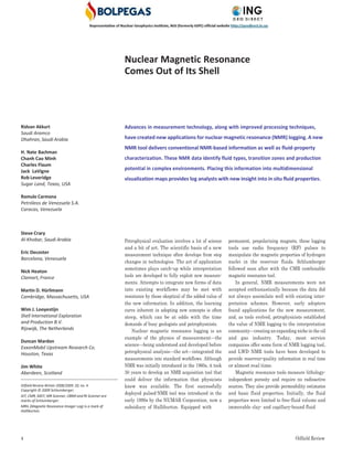
3. 6 Oilfield Review
B
Antenna
WT
> Basic NMR theory. Hydrogen nuclei behave like tiny bar magnets and tend to align with the
magnetic field of permanent magnets, such as those in an NMR logging tool (A). During a set wait
time (WT), the nuclei polarize at an exponential buildup rate, T1, comprising multiple components (C).
Next, a train of RF pulses manipulates the spins of the hydrogen nuclei causing them to tip 90° and
then precess about the permanent magnetic field. The formation fluids generate RF echoes between
successive pulses, which are received and measured by the antenna of the NMR tool (B). The time
between pulses is the echo spacing (TE) (D). The amplitudes of the echoes decay at a superposition
of exponential relaxation times, T2, which are a function of the pore-size distribution, fluid properties,
formation mineralogy and molecular diffusion (E). An inversion technique converts the decay curve
into a distribution of T2 measurements (F). In general, for brine-filled rocks, the distribution is related
to the pore sizes in the rocks (G).
Echo TE
CPMG sequence
After a given WT, a train of electromagnetic
RF pulses manipulates the magnetic moments of
the hydrogen nuclei and tips their direction away
from that of the B0 field. The process of sending
long trains of RF pulses is referred to as a CPMG
sequence.2
A key feature of this sequence is
alternating the polarity of the received signal to
eliminate electronics-related artifacts. During
the CPMG measurement cycle, the hydrogen
nuclei in the formation generate detectable RF
echoes at the same frequency used to manipulate
them.3
The echoes occur between RF bursts. The
time between bursts is the echo spacing, TE.
The amplitude of the echoes is proportional
to the net magnetization in the plane transverse
to the static field created by the permanent
magnets. The amplitude of the initial echo is
directly related to the formation porosity. The
strength of the subsequent echoes decreases
exponentially during the measurement cycle.
The exponential decay rate, represented by the
relaxation rate, T2, is primarily a function of pore
size, but also depends on the properties of the
fluid in the reservoir, the presence of
paramagnetic minerals in the rock and the
diffusion effects of the fluids. In typical cases,
the decay of the echo amplitudes is governed by
a distribution of T2 times, similar to the T1 times
found in the buildup curve. An inversion
technique fits the decay curve with discrete
exponential solutions. These solutions are
converted to a continuous distribution of
relaxation times representative of the fluid-filled
pores in the reservoir rock (above).4
When the fluid in the sensed region is brine,
the T2 distribution is generally bimodal,
particularly in sandstones. Small pores and
bound fluid have short T2 times, and free fluids
in larger pores have longer relaxation times. The
dividing line between bound and free fluid is
referred to as the T2 cutoff. Oil and gas in the
pore spaces introduce a few complications into
the model.
The three primary mechanisms that
influence T2 relaxation times are grain surface
relaxation, relaxation by bulk-fluid processes and
relaxation from molecular diffusion.5
Grain
surface relaxation is a function of pore-size
distribution. Relaxation effects from molecular
diffusion and bulk-fluid properties are directly
related to the type of fluid in the pores.
Tar has an extremely short relaxation time
and may not be measurable with downhole NMR
tools. Heavy oils have short relaxation times,
similar to those of clay- and capillary-bound
fluids, but may also be too short for NMR
acquisition (next page). Lighter oils have longer
T2 times, similar to those associated with free
fluids. Gas has an even longer relaxation time
than oil. During the measurement process, oil
and gas signals are detected along with signals
from movable and irreducible water. While the T2
times from the oil and gas signals may have no
relationship to the producibility of the
Time
T2
Amplitude
Amplitude
Amplitude

4. Winter 2008/2009 7
Brine T2 Distributions Oil T2 Distributions Total Distribution
Pore size Viscosity and composition
> The effects of oil on T2 distributions. For brine-filled pores, the T2
distribution generally reflects the pore-size distribution of the rock. This
distribution is often bimodal, representing small and large pores (left). The
small pores contain clay- and capillary-bound fluids and have short
relaxation times. The large pores contain movable free water and have
longer relaxation times. The dividing line between bound and free fluids is
the T2 cutoff. When oil fills the reservoir pore spaces, the measured T2
distribution is determined by the viscosity and composition of the oil
(middle). Because of their molecular structure, tar and viscous heavy oils
have fast decay rates, or short T2 times. Lighter oils and condensate have a
spectrum of T2 times, overlapping with those of larger brine-filled pores.
Mixed oil and water in the reservoir result in a combination of T2 times
based on both pore size and fluid properties (right).
hydrocarbons, they do help characterize the fluid
type. Techniques have been developed to exploit
the fluid response and identify the presence and
type of hydrocarbons.
In the past, there were two primary tech-
niques by which NMR data were used to identify
fluids: differential spectrum and enhanced
diffusion.6
The differential spectrum technique
combines measurements with two different wait
times. Short WTs underpolarize formation fluids,
such as gas and light oil, which have long buildup
and decay times. Measurements from fluids with
short relaxation times are not affected by a
change in WT. Differences between sequential
logging passes identify the presence of light
hydrocarbon, making the differential spectrum
technique most effective in gas or condensate
environments. Logging sequences have also been
developed that acquire the data in a single pass.
Enhanced diffusion exploits changes in fluid
response that occur when different echo spacings,
or TEs, are used.7
Water and oil generally have
similar relaxation times when measurements are
2. CPMG refers to the physicists who successfully deployed
the RF pulse sequence used in NMR devices—
Herman Carr, Edward Purcell, Saul Meiboom and
David Gill.
3. During the CPMG sequence, hydrogen atoms are
manipulated by short RF bursts from an oscillating
electromagnetic field. The frequency of the RF pulses is
the Larmor frequency.
4. Freedman R and Heaton N: “Fluid Characterization Using
Nuclear Magnetic Resonance Logging,” Petrophysics 45,
no. 3 (May–June 2004): 241–250.
5. Kleinberg RL, Kenyon WE and Mitra PP: “On the Mechanism
of NMR Relaxation of Fluids in Rocks,” Journal of
acquired using short TEs, but water often relaxes
faster than oil when longer TEs are used. To
isolate the oil signal, a measurement with a short
TE is compared with an echo train with a longer
TE, chosen to enhance the diffusion differences of
the fluids in the formation. The water signal
decreases with longer TEs, leaving primarily the
oil signal. This diffusion sensitivity provides a
qualitative indication of the presence of oil,
although the measurement may sometimes be
quantitative as well.8
Both differential spectrum and enhanced
diffusion rely on traditional T2 relaxation
measurements to identify hydrocarbons. This
limits the results to a one-dimensional aspect of
the fluids, and fluid type can only be inferred, not
directly quantified. Also, prior knowledge of the
expected fluids is necessary to choose the correct
acquisition parameters. The primary limitation of
the relaxation dimension is the difficulty in
distinguishing water from oil (see “Dimensions in
NMR Logging,” next page). But, the fact that oil
and gas signals are included with the water signal
Magnetic Resonance 108A, no. 2 (1994): 206–214.
6. Akkurt R, Vinegar HJ, Tutunjian PN and Guillory AJ:
“NMR Logging of Natural Gas Reservoirs,” The Log
Analyst 37, no. 6 (November–December 1996): 33–42.
7. Akkurt R, Mardon D, Gardner JS, Marschall DM and
Solanet F: “Enhanced Diffusion: Expanding the Range of
NMR Direct Hydrocarbon-Typing Applications,”
Transactions of the SPWLA 39th Annual Logging
Symposium, Houston, May 26–29, 1998, paper GG.
8. Looyestijn W: “Determination of Oil Saturation from
Diffusion NMR Logs,” Transactions of the SPWLA 37th
Annual Logging Symposium, New Orleans, June 16–19,
1996, paper SS.
in the total distribution introduces an exploitable
dimension to the relaxation distributions. Remove
the water contribution and only the hydrocarbon
signal remains.
Molecular diffusion is the key to unlocking
fluid properties from the NMR data. Gas and
water have characteristic diffusion rates that can
be calculated for given downhole conditions. Oil
has a range of diffusion values based on its
molecular structure. This range can also be
predicted from empirical data derived from
dead-oil samples.
The T2 measurement provides the total
volume of fluid—bound and free. The addition of
diffusion discriminates the type of fluid present.
A graphical presentation—the diffusion-T2, or
D-T2, map—displays these data in a 2D space
formed by the diffusion dimension and the
relaxation dimension. The water signal can be
separated from that of the hydrocarbons. The
intensity of the components in the D-T2 map
provides fluid saturations. Maps can also be
generated using T1 relaxation data.
This quantification of diffusion is made
possible by a new acquisition technique,
diffusion editing (DE), which alleviates the
limitations of previous methods, such as
enhanced diffusion and differential spectrum.
Distinguishing water and hydrocarbon by their
diffusivity differences not only permits the
(continued on page 13)

5. 8 Oilfield Review
Dimensions in NMR Logging
> T1 logging. Traditional NMR CPMG sequences measure T2 distributions and begin after a
sufficient WT for polarization of hydrogen nuclei. For T1 acquisition, a succession of short CPMG
cycles with WTs selected over a range of values is used. In a departure from earlier T1 acquisition
methods, the MR Scanner tool acquires full T2 echo trains for each chosen WT value, and thus
the resulting data can be subjected to a multidimensional inversion and provide both T1 and T2
distributions. T1 logging is especially useful in low signal-to-noise environments and for fluids
with long polarization times, such as are found with light hydrocarbons and in large pores. In
addition, T1 distributions, unlike T2 distributions, are free of diffusion effects and provide more-
accurate results in highly diffusive fluids.
T2 component. In practice, a 2D inversion
directly transforms the original echo dataset
to a 2D T1-T2 distribution, sometimes referred
to as a T1-T2 map (next page, top left).3
For many fluids, T1 and T2 distributions are
very similar since they are governed by the
same physical properties. Under typical
measurement conditions the T1/T2 ratio for
water and oil ranges between 1 and 3.
However, an important difference between
the two relaxation times is that T2 times are
affected by molecular diffusion whereas T1
times are free of diffusion effects. In NMR
measurements, diffusion causes a reduction
in echo amplitude and therefore shortens T2
times. The magnitude of the diffusion effect
is a function of the molecular-diffusion
constant of the fluid, D, and the echo
spacing, TE. TE is an adjustable
measurement parameter defining the time
between consecutive radio frequency (RF)
pulses in the measurement sequence.
Diffusivity is an intrinsic fluid property,
Humans generally visualize in three dimensions,
and geometric relationships are understood
as adding levels of complexity with each
dimension. For instance, a 1D image may have
length, 2D adds width, 3D adds depth, and 4D
adds the element of time.1
Analogous to
spatial relationships, NMR measurements can
be described using dimensionality, with each
dimension adding a degree of complexity.
The 1D NMR distribution refers to T2
transverse relaxation time measurements. T2
distributions are obtained by inverting raw
NMR echo-decay signals. The distributions
contain information about both fluid
properties and pore geometry. However,
signals from different fluids often overlap,
and it is not always possible to distinguish
water from oil, or water from gas purely on
the basis of the T2 distribution.
The T1 relaxation measurement, from the
buildup of polarization, also provides a 1D
distribution. A single echo (or a small number
of echoes) is acquired for a series of different
wait times, WTs.2
The observed increase in
echo amplitude with increasing WT is the
polarization buildup, which is governed by the
distribution of T1 relaxation times (above).
With a mathematical inversion similar to the
one employed to derive T2 distributions from
echo-decay signals, the T1 distribution is
extracted from the polarization buildup.
During the T1 acquisition, a full T2 echo-
decay signal can be acquired for each WT,
rather than a single echo or a short series of
echoes, and thus a 2D dataset can be
generated with T2 and T1 data. The individual
echo-decay signals are inverted to obtain a
separate T2 distribution for every WT. Each T2
component follows its own characteristic
buildup with increasing WT, governed by the
T1 distribution (buildup) associated with that
depending only on the fluid composition,
temperature and pressure. Once quantified, it
identifies the fluid type.4
For water, D is
primarily related to temperature, and for
natural gas, it is determined by both tempera-
ture and pressure. Crude oils exhibit a
distribution of diffusion rates governed by the
molecular composition, temperature and
pressure. Diffusion, therefore, is the key to
identifying fluid type with NMR. For example,
T2 relaxation times for gas are much shorter
than T1 times because of diffusion. By
identifying the difference between T1 and T2
measurements in a gas reservoir, the
hydrocarbon type can be inferred.
Diffusion distributions are determined by
measuring echo-amplitude decays for echo
trains acquired with different echo spacings,
TEs. However, increasing the TE to allow
diffusion to take place comes at a price. The
increased time between echoes means there
Polarization

6. Winter 2008/2009 9
> Two-dimensional NMR data. The 2D nature
of T1-T2 maps is highlighted by overlapping
signals from the two sets of distributions. The
crossplotted signals are at maxima, indicated
by the color variation from blue to dark red, in
the center and right of this plot. The data
converge along the center line in the middle—
their agreement indicating similar fluid
measurements from both T1 and T2. But,
divergence of the longer time components of
the two sets of data, resulting from molecular
diffusion, moves the plot away from the center
line at the right corner. If there were no
diffusion effects, the crossplot would be
centered along the dividing line.
> Diffusion editing. With traditional CPMG sequences and short echo spacing (TE), oil (green)
and water (blue) signals relax, or decay, at similar rates (top). Lengthening the TE value (middle)
enhances the diffusion effect preferentially for the fast-diffusing water compared with slower-
diffusing oil. However, long TEs correspond to fewer echoes and a lower signal-to-noise ratio.
Diffusion editing (bottom) is a variant of the multi-TE CPMG method, where only the first two
echoes are lengthened to enhance the diffusion effect, while maintaining the advantage of the
short TE for better signal-to-noise ratio.
are fewer echoes over an equivalent time
span, reducing the data density. This also
results in more rapid signal decay—T2 times
are shorter—because of the diffusion effects.
The end result is a reduction in the amount of
usable data, and the inversion becomes more
challenging because of the lower signal-to-
noise ratio.
The diffusion-editing (DE) technique
overcomes these limitations by combining two
long initial TEs—during which diffusion is
effective in reducing the NMR signal—
followed by an extended train of short TEs,
during which diffusion effects are minimized
(above right). A large number of echoes can
be acquired, and the effective signal-to-noise
ratio is maximized.
Analogous to the T1-T2 measurement
described earlier, a 2D experiment can be
designed to extract diffusion information.
1. Beyond classical physics, there are other applications
that describe four dimensions and beyond. String
theory, for example, predicts 10 dimensions, including
a zero dimension.
2. The wait time is the time allotted for the alignment
of protons within the static magnetic field of the
permanent magnet of an NMR logging tool during the
measurement cycle.
Rather than acquiring echo trains for a
number of sequential WTs, an echo train is
acquired with different initial long TEs. The
data are subjected to the inversion processing
and can then be used to generate D-T2 maps,
3. Song YQ, Venkataramanan L, Hürlimann MD, Flaum M,
Frulla P and Straley C: "T1–T2 Correlation Spectra
Obtained Using a Fast Two-Dimensional Laplace
Inversion,” Journal of Magnetic Resonance 154, no. 2
(February 2002): 261–268.
4. Freedman and Heaton, reference 4, main text.
T1 T2

7. 10 Oilfield Review
> D-T maps. Diffusion plotted with T2 (or T1) provides 2D reservoir-fluid maps that can resolve oil,
gas and water. In this example, the diffusion dimension (right) is the key to identifying the fluids,
which otherwise overlap in the T2 dimension (top left ). The amplitudes of the signals along one
direction of the two-dimensional map result in 1D distributions, which then can be converted to
fluid saturations. As an aid to interpreting the 2D maps, fluid-diffusion coefficients are
superimposed on the map (bottom left). The gas line (red) is computed using downhole pressure
and temperature inputs. The water line (blue) is calculated using the downhole formation
temperature. The oil line (green) shows the position of oil at different viscosities, with the lower
left being heavy oil, trending to light oil and condensate at the upper right. The interpretation of
this map is that the reservoir contains gas, oil and water.
T2, which contains important complementary
information about composition, such as
gas/oil ratio (GOR) and pore-size information
for water, cannot be measured. This limitation
is overcome by invoking a third dimension to
combine with diffusion, T1 relaxation times.6
The 3D NMR measurements acquire echo-
train data at multiple WTs (for T1) and
multiple TEs (for diffusion). Sufficient
information is then available to create 3D
maps of D-T1-T2, in which the T2 axis refers to
a transverse relaxation time with diffusion
effects removed (next page, left). The map is
therefore a 3D correlation of intrinsic fluid
properties for T1, T2 and D. In practice, NMR
fluid maps are typically presented in a 2D
format, plotting D with either T1 or T2, or on
occasion plotting T1 with T2.
Overlain on the maps are default fluid-
response lines for the D of gas and water
computed from their diffusion coefficient at
formation temperature and pressure. The oil
line is derived from the estimated dead-oil
response at downhole conditions.
The fourth dimension in NMR logging, the
radial distance from the borehole wall, results
from acquisition at multiple depths of
investigation (DOIs). Data from two or three
DOIs are simultaneously inverted. Results
from the shallow DOI are used to correct data
from deeper DOIs, improving the outputs
affected by missing information and poorer
signal-to-noise ratios.
NMR logging tools acquire data from a
region often affected by filtrate invasion,
which alters the original fluid distribution.
The 4D NMR processing is based on the
which are a graphical means to identify fluid
type and quantify saturations (above).5
Although the two-dimensional D-T2
measurement is effective in separating the oil
signal from that of the water, it is less robust
for distinguishing between highly diffusive
5. Hürlimann MD, Venkataramanan L, Flaum C, Speier P,
Karmonik C, Freedman R and Heaton N: “Diffusion-
Editing: New NMR Measurement of Saturation and
Pore Geometry,” Transactions of the SPWLA 43rd
Annual Logging Symposium, Oiso, Japan, June 2–6,
2002, paper FFF.
6. Freedman and Heaton, reference 4, main text.
7. Cao Minh C, Heaton N, Ramamoorthy R, Decoster E,
White J, Junk E, Eyvazzadeh R, Al-Yousef O, Fiorini R
fluids, such as gas, condensate or water at
high temperatures. The problem arises
because diffusion can dominate the T2
relaxation mechanism for these fluids, even at
the shortest echo spacing available from the
logging tools. The underlying “diffusion-free”
and McLendon D: “Planning and Interpreting NMR
Fluid-Characterization Logs,” paper SPE 84478,
presented at the SPE Annual Technical Conference
and Exhibition, Denver, October 5–8, 2003.
8. For more on wettability: Abdallah W, Buckley JS,
Carnegie A, Edwards J, Herold B, Fordham E, Graue A,
Habashy T, Seleznev N, Signer C, Hussain H, Montaron B
and Ziauddin M: “Fundamentals of Wettability,”
Oilfield Review 19, no. 2 (Summer 2007): 44–61.
assumptions that bound-fluid volume and
immovable hydrocarbon volume are invariant
to DOI. The shallow-measurement data are
used to constrain the inversion for the deeper
measurements by fixing the bound-fluid
components. (For examples of 4D NMR
processing, see pages 16 and 17.) Diffusion
and T1 (or T2) data from 4D NMR are used to
produce fluid maps at multiple DOIs. Fluid
changes that take place as filtrate invades the
reservoir rock are graphically displayed and
Gas
Gas diffusion
coefficient
coefficient
Gas

8. Winter 2008/2009 11
> Three dimensions of NMR. Diffusion, T1
distributions and T2 distributions presented in
a 3D format provide intrinsic fluid properties.
The cube is used to identify diffusion effects
and may aid the interpreter in deciding which
model best describes the fluid properties.
> NMR in four dimensions. The fourth dimension of NMR logging is depth. Bound-fluid volumes,
associated with both clay- and capillary-bound fluids (yellow), do not generally change when
filtrate from the drilling fluid invades the reservoir. Tool or measurement limitations, however, can
result in changes in computed fluid properties that do not represent the true fluid distributions.
Constraining the volumes of bound fluid measured by deeper-reading shells to be equivalent to
that of the more-precise shallower shells and reapportioning the total porosity across the fluid
spectrum provide more-accurate fluid analysis. Use of 4D NMR processing is especially
beneficial in interpreting data from heavy-oil reservoirs.
allow petrophysicists to detect oil mobility,
wettability effects and fluid interactions
(above right).
Although the interpretation of maps created
from 3D or 4D NMR data might seem simple,
complications do exist. The results rely on a
forward-model approach that assumes the
fluid and the reservoir meet certain criteria.
When nonideal fluid properties or atypical
reservoir conditions are encountered, the
response deviates from the model, and
conflicting or erroneous results may ensue.7
In some cases, nonideal effects can be
detected and even quantified by inspection
of the D-T maps. Relevant parameters in the
forward model can be adjusted once these
effects are identified.
In another problem, when diffusion of fluid
molecules in small pores is restricted, the
measured values of diffusion are reduced
from those of the ideal model (next page).
While the signal from fluids in large pores
appears as expected in the D-T maps, fluids
in the small, poorly connected pores may plot
at lower diffusivity values. The problem is
most common for water diffusion in fine-
grained carbonate rocks. If the effect is not
identified, the calculated oil saturation may
be overly optimistic. However, once the
restricted-diffusion effect is detected, model
parameters can be adjusted according to the
observed 2D map results and fluid-saturation
estimations corrected.
Another anomalous effect results from
internal magnetic-field gradients caused by
paramagnetic and ferromagnetic materials in
the rocks, either in the matrix or coating the
grains. These are often associated with high
chlorite content and create significant
localized field gradients, resulting in faster
relaxation times. Because the inversion model
is based on the tool’s fixed magnetic-field
gradient, the D-T map responses of the fluids
in these rocks are shifted to higher diffusion
rates, the opposite of the restricted-diffusion
effect. For example, water signals may appear
above the water line. Fortunately, it is usually
possible to identify these effects by inspection
of the maps, and model parameters can then
be adjusted to provide correct interpretations.
The wettability state also affects D-T maps.
Under water-wet conditions, the oil viscosity
determines the position of the oil signal along
the oil line of the map. The trend is from
heavy oil at the bottom left to lighter oils and
condensate at the top right of the line. Oil-
wet rocks and those with mixed wettability
tend to have shorter relaxation times because
of the additional surface relaxation of the
hydrocarbon in direct contact with the pore
surface. Although this can compromise the
accuracy of oil viscosity estimated from the
NMR data, it can also be a useful
measurement for petrophysicists in
understanding the nature of the reservoir.8
Amplitude

9. 12 Oilfield Review
Internal
gradient
High
GOR
OBMF
with gas
Bound
water
Native
oil
Internal
gradient
Water
High
GOR
diffusion
Restricted
diffusion
Restricte
d
diffusion
> Interpreting the maps. After inversion, two-dimensional crossplots of
the data identify the presence of oil, water and gas. When the plot of
the response from formation fluids (shown as color contours) conforms
to the interpretation model, the response will fall on or near the
expected gas, oil or water lines. This affords a straightforward
interpretation. Water falls on the water line as shown (middle).
However, signals frequently fall off the lines as a result of competing
petrophysical effects, which include internal gradients, restricted
diffusion, wettability and high gas/oil ratios (GOR). Because internal
gradients shorten the relaxation times, the plots tend to shift upward
(top left ). Restricted diffusion causes the measured diffusion rate to
increase, and, as a consequence, the plots will trend down and away
from the expected fluid line (bottom left). Plots from oil-wet reservoirs
tend to shift to the right of the oil line, as do reservoirs with mixed
wettability (bottom right). The maps from oil-wet and mixed-wet
reservoirs tend to have a spectrum of responses, which produce a
broader image. Because the model is built with dead-oil responses,
maps from high-GOR oil reservoirs may not respond as expected. These
plots are shifted away from the oil line toward the gas line (top right). In
a reservoir that contains only gas, OBM filtrate may mix with the native
gas and produce a response similar to that of high-GOR oil. Deeper
measurements often help experts refine their interpretation of these
maps because filtrate generally diminishes away from the wellbore and
gas response increases.
Fluids with a high GOR tend to plot above
and to the left of the oil line. This can be seen
in native fluids and gas-bearing zones invaded
by oil-base mud filtrate (OBMF). OBMF
should plot as a moderate to light hydrocarbon.
The response of OBMF mixed with native gas
from the reservoir plots between the oil and
water lines.
The D-T maps are powerful tools for inter-
preting fluid types in the reservoir. In many
cases the interpretation is straightforward, but
consideration must be given to external factors
that lead to nonideal behavior and mislead a
novice interpreter. For this reason, it is
important to rely on experts adequately trained
in processing and interpreting NMR data.
A surgeon relies on a trained radiologist to
interpret MRI images. A clean break of a bone
is easy to spot, even by a novice user, but
experience helps a radiologist differentiate
between bone fragments and calcification.
The differences may be indistinguishable to
the untrained eye. In a similar manner, the
log analyst may easily determine the presence
of water or gas in a D-T map, but there are
occasions when a skilled NMR expert should
be called in to help analyze the results. With
the aid of fluid maps and an understanding of
the measurement physics, the petrophysicist
can diagnose conditions that are hidden from
the inexperienced observer.

10. Winter 2008/2009 13
computation of fluid saturations, but also helps
infer fluid viscosity from the T2 contribution of
the fluid (right).
Diffusion-editing sequences from the new
MR Scanner service supply a water-saturation
output that is independent of that traditionally
derived from resistivity and porosity measure-
ments. In contrast to a saturation derived from
Archie’s equation, NMR-based saturation
measurement techniques are useful in fresh
water or formation waters of unknown salinity.
Wettability can also be inferred from NMR data.
One drawback to using NMR measurements for
fluid characterization is that the measurement
comes from a near-well region referred to as
the flushed zone, where mud-filtrate effects are
strongest.
10
1
0.1
0.01
0.001
0.0001
0.1
1 10 100
Viscosity, cP
1,000 10,000 100,000
The MR Scanner Tool
Although NMR measurements may come from
only a few inches into the formation, they can still
provide formation-fluid properties. To measure
continuous in situ fluid characteristics—
including fluid type, volume and oil viscosity—
much more information is needed than was
provided by previous-generation NMR tools.9
For
this reason, fluid characterization was a key driver
in the development of the MR Scanner service.
In the past, there were two basic designs for
NMR tools: pad-contact tools and centralized
concentric-shell tools. The pad device, represented
by the CMR tool, measures NMR properties of a
cigar-sized volume of the reservoir fluids at a
fixed depth of investigation (DOI) of approxi-
mately 1.1 in. [2.8 cm]. The NUMAR MRIL
Magnetic Resonance Imager Log tool measures
concentric cylindrical resonant shells of varying
thickness and at fixed distances from the tool,
with the DOI determined by hole size and tool
position in the wellbore.
The MR Scanner design offers the fixed DOI
of a pad device with the flexibility of multiple
DOIs of resonant shells.10
It consists of a main
antenna optimized for fluid analysis and two
shorter high-resolution antennas best suited for
acquiring basic NMR properties (right). The
main antenna operates at multiple frequencies
corresponding to independent measurement
volumes (shells) at evenly spaced DOIs.
9. Heaton NJ, Freedman R, Karmonik C, Taherian R,
Walter K and DePavia L: “Applications of a New-
Generation NMR Wireline Logging Tool,” paper
SPE 77400, presented at the SPE Annual Technical
Conference and Exhibition, San Antonio, Texas,
September 29–October 2, 2002.
10. DePavia L, Heaton N, Ayers D, Freedman R, Harris R,
Jorion B, Kovats J, Luong B, Rajan N, Taherian R,
Walter K, Willis D, Scheibal J and Garcia S: “A Next-
Generation Wireline NMR Logging Tool,” paper
SPE 84482, presented at the SPE Annual Technical
Conference and Exhibition, Denver, October 5–8, 2003.
> Viscosity transform. The T2 (or T1) relaxation time for crude oil is a function
of viscosity. The relaxation time can be converted to viscosity using an
empirically derived transform. Because of diffusion effects, the viscosity
measurement for heavy oils below 3 cP [0.003 Pa.s] is influenced by the echo
spacing (TE) of the measurement. Thus, T2 times may be tool dependent for
heavy oils if the tool is not capable of shorter TEs. As a consequence of
diffusion, T1 and T2 values in light oils diverge above 100 cP [0.1 Pa.s].
> MR Scanner service. The MR Scanner tool has three antennas. The main antenna operates at
multiple frequencies and is optimized for fluid-property acquisition. The sensed region consists of
very thin shells that form arcs of approximately 100° in front of the 18-in. [46-cm] length of the antenna.
The thickness of the individual shells is 2 to 3 mm. The two high-resolution antennas are 7.5 in. [19 cm]
long and provide measurements with a DOI of 1.25 in. [3.17 cm]. The MR Scanner tool is run eccentered
with the antenna section pressed against the borehole.
T
1
or
T
2
,
s
High-resolution
antennas
Main antenna

11. 14 Oilfield Review
> Gradient tool and DOI. The MR Scanner tool is referred to as a gradient
tool because the magnetic-field strength (B0, blue) from the permanent
magnet, although uniform over the sample region, decreases monotonically
away from the magnet. The tool’s magnet extends along the length of the
sonde section. A constant, well-defined gradient simplifies fluid-property
measurements. The DOI is determined by the magnetic-field strength and the
frequency of RF operation, f0 . Although multiple frequencies are available
from the tool, standard operating procedure is to acquire data from the 1.5-in,
2.7-in. and 4.0-in. DOI shells, referred to as Shell No. 1, Shell No. 4 and
Shell No. 8, respectively. Three shells are shown, with their respective DOI-
related operating frequencies. The frequency associated with Shell No. 1 is
shown in green.
Borehole rugosity and thick mudcake can invali-
date shallow NMR measurements but rarely affect
the readings from the deeper shells. NMR porosity
from a deep shell has been used as a substitute for
formation density porosity when that measure-
ment was compromised by borehole rugosity.
Fluid-property changes resulting from mud-
filtrate invasion may also be observed and
quantified using radial profiling. Often more than
just filtrate from the drilling mud invades the
formation. Whole mud and mud solids can
replace existing fluids in the near-wellbore
region. NMR-derived porosity and permeability
may be reduced by the presence of these solids,
but the effects diminish deeper into the
formation. Radial profiling identifies and
overcomes these effects.
Saturation profiling delivers advanced fluid-
characterization measurements such as oil, gas
and water saturations, fluid type and oil
viscosity—all at discrete multiple DOIs. One
application of saturation profiling is the
evaluation of heavy-oil reservoirs.
Viscosity and Rugosity
Of the world’s known reserves, 6 to 9 trillion
barrels [0.9 to 1.4 trillion m3
], are found in the
form of heavy- or extraheavy-oil accumulations.11
This is triple the amount of world reserves of
conventional oil and gas combined. Heavy-oil
reservoirs pose serious operational concerns for
Although multiple frequencies are available
from the main antenna, the three most
commonly used are Shells No. 1, No. 4 and No. 8,
which correspond to 1.5-in., 2.7-in. and 4.0-in.
Shell No. 8
Shell No. 4
Shell No. 1
> Radial profiling. The MR Scanner tool senses
fluid from multiple, thin DOI shells. The spacing is
optimized to avoid shell interaction. Fluid
properties vary in the first few inches into the
formation as a result of flushing by mud filtrate.
Deeper shells are less affected by filtrate, mud
invasion and borehole rugosity than are shallow-
reading shells.
[3.8-cm, 6.8-cm and 10.2-cm] DOIs, respectively.
A recently introduced three-shell simultaneous
acquisition mode eliminates the need for multiple
passes to acquire data from all three DOIs.
Profiling Fluid Properties
The three primary frequencies commonly used by
the MR Scanner tool correspond to three
independent DOIs, providing measurements at
discrete radial steps into the formation. The
frequency of the RF pulse, along with the field
strength of the magnet, determines the DOI of
the shell (above). A key advantage of the MR
Scanner shells is that the measurement comes
from a thin cylindrical portion of the formation—
an isolated slice—and is not generally affected by
the fluids between the tool and the measurement
volume. This allows interpretation of near-
wellbore fluid properties in a manner that is
unique in formation evaluation.
Multiple DOIs introduce new concepts for
NMR logging—radial profiling and saturation
profiling (left). Profiling incorporates
measurements from successive DOIs to quantify
changes in fluid properties occurring in the first
few inches of formation away from the wellbore.
proper evaluation of fluids and production
potential. Sampling with wireline-conveyed tools
or drillstem tests may not be possible because of
the difficulties in getting the oil to flow. NMR
measurements can provide essentialinformation
on in situ fluid properties to evaluate heavy-oil
reservoirs.
Located south of the Eastern Venezuelan
basin, the Orinoco heavy-oil belt holds an
estimated 1.2 trillion barrels [190 billion m3
] of
heavy oil. NMR logs have been an integral part of
evaluation programs of the wells drilled in this
region, but with recognized limitations.12
The
relaxation times of high-viscosity oils are very
short and may not be fully measurable using
NMR tools. Also, borehole conditions in the
Orinoco basin are often poor, with rugosity that
affects pad-contact tools.
Although the early introduction of NMR fluid
characterization with the CMR tool showed
promise, the measurements were limited to a
single, shallow DOI. Techniques were developed
to use NMR data to estimate the oil viscosity
throughout a sand interval based on the
logarithmic mean of T2 distributions. Encouraging
DOI
Decreasing B0 strength
Borehole
ƒ0
Main
Distance from magnet
No. 4 Shell
Shell
No. 1
Magnet

12. Winter 2008/2009 15
X,200
X,250
Resistivity
10-in. Array
0.2 ohm.m 2,000
20-in. Array
0.2 ohm.m 2,000
30-in. Array
0.2 ohm.m 2,000 Heavy Oil Heavy Oil Heavy Oil Permeability
60-in. Array
0.2 ohm.m 2,000
Free Water Free Water Free Water Shell No. 1
100,000 mD 1
Oil Oil Oil
Caliper
6 in. 16
90-in. Array
0.2 ohm.m 2,000
T1 Distribution,
Shell No. 1
T1 Distribution,
Shell No. 4
T1 Distribution,
Shell No. 8
Shell No. 4
100,000 mD 1
Bound Water Bound Water Bound Water
Depth
ft
RXO
0.2 ohm.m 2,000
T1 Cutoff
1 ms 9,000
T1 Cutoff
1 ms 9,000
T1 Cutoff
1 ms 9,000
Porosity, Shell No. 1
40 % 0
Porosity, Shell No. 4
40 % 0
Porosity, Shell No. 8
40 % 0
Shell No. 8
100,000 mD 1
X,100
X,150
X,200
X,250
> Radial profiling with filtrate and whole-mud invasion. The interval from
X,170 to X,255 ft (red shading) is a clean water sand beneath a heavy-oil
reservoir in the Orinoco heavy-oil basin. The fluid properties from the
1.5-in. DOI, Shell No. 1 (Track 5) have spurious volumes of bound water
(light brown). Even at 2.7 in., Shell No. 4 indicates more bound fluid than
expected for a clean sand (Track 6, light brown). The differences are
attributed to whole-mud invasion. The Shell No. 8 data come from a region
beyond the whole-mud invasion and provide more-representative
information (Track 7). The total porosity measurements from the three shells
appear to be unaffected by the presence of whole mud. Permeabilities
calculated from the shallower shells (Track 8, blue, green) are lower than
that of the deepest shell (Track 8, red) because the measurements are
affected by the solids that are filling the pore spaces.
results were obtained but fell short of true in situ
viscosity. There was no calibrated transform to
link the logarithmic mean of the T2 distributions
to the viscosity at downhole conditions that would
also account for the apparent hydrogen index (HI)
of the oil.13
The importance of using HI and an
empirical transform was demonstrated by recent
laboratory work.14
The MR Scanner tool was included in a more
recent logging program, in part, to overcome some
of the limitations of the CMR measurements.
Radial profiling was found to be beneficial in
zones where rugosity affected the 1.5-in. DOI
measurement from Shell No. 1, which is
comparable to the CMR tool’s DOI. The 2.7-in.
measurement from Shell No. 4 was only slightly
11. Alboudwarej H, Felix J, Taylor S, Badry R, Bremner C,
Brough B, Skeates C, Baker A, Palmer D, Pattison K,
Beshry M, Krawchuk P, Brown G, Calvo R, Cañas Triana JA,
Hathcock R, Koerner K, Hughes T, Kundu D, López de
Cárdenas J and West C: “Highlighting Heavy Oil,”
Oilfield Review 18, no. 2 (Summer 2006): 34–53.
12. Decoster E and Carmona R: “Application of Recent NMR
Developments to the Characterization of Orinoco Belt
Heavy Oil Reservoirs,” Transactions of the SPWLA 49th
Annual Logging Symposium, Edinburgh, Scotland,
May 25–28, 2008, paper VVV.
affected by rugosity. The 4.0-in. Shell No. 8 data
were not affected because they were acquired from
a region beyond the rugosity (above).
13. Carmona R and Decoster E: “Assessing Production
Potential of Heavy Oil Reservoirs from the Orinoco Belt
with NMR Logs,” Transactions of the SPWLA 42nd
Annual Logging Symposium, Houston, June 17–20, 2001,
paper ZZ.
14. Burcaw L, Kleinberg R, Bryan J, Kantzas A, Cheng Y,
Kharrat A and Badry R: “Improved Methods for
Estimating the Viscosity of Heavy Oils from Magnetic
Resonance Data,” Transactions of the SPWLA 49th
Annual Logging Symposium, Edinburgh, Scotland,
May 25–28, 2008, paper W.

13. 16 Oilfield Review
Caliper 50 % 0 50 % 0 25 % 0
> 4D NMR processing. Standard processing results in a lack of coherence between bound-fluid volumes measured
by Shells No. 1, No. 4 and No. 8 (top, Track 1). The same is true for the free-fluid volumes (Track 3). Using 4D NMR
processing, the bound-fluid volumes, which should remain constant across each DOI, are constrained and the
porosity contributions are reassigned. The result is improved coherence for both the bound-fluid (Track 2) and free-
fluid (Track 4) volumes. The fluid properties are affected by hole conditions from X,120 to X,135 ft (red shading) as
evidenced by the increased porosity measured from the shallower shells (Tracks 5, 6, 8 and 9). Shell No. 8 (Tracks 7
and 10) senses from beyond the washout and provides more-accurate data. The D-T1 maps used for saturation
computation for each shell demonstrate the effectiveness of 4D processing. The standard 2D NMR processing
(bottom left panel) results in similar fluid volumes in Shells No. 1 and No. 4. Shell No. 8 has less bound fluid, but all
three shells should have equivalent volumes because bound fluid should not change with DOI. The 4D NMR
processing (bottom right panel ) constrains the fluid volume to be the same below 30 ms. Reapportioning the
porosity to account for the bound-fluid volume delivers a more-accurate measurement from the deepest shell. As a
result, the 4.0-in. measurement furnishes fluid properties from a region less influenced by mud-filtrate invasion.
The independent measurements at various
DOIs from the MR Scanner tool read deeper into
the formation than the CMR tool. Not only has the
MR Scanner tool overcome rugosity problems, it
also has verified a condition—previously
theorized from the CMR data—of partial- or
whole-mud invasion effects on the bound-fluid
volumes and permeability. These effects were
especially noticeable in water zones. The mud
solids did not appreciably alter NMR porosity, but
the bound-fluid measurement was too high. As an
input to the NMR permeability calculation,
incorrect bound-fluid volume resulted in
permeability outputs that were too low.
Deeper-reading NMR measurements overcome
rugosity but have some trade-offs. Because the
formation signals from the deeper shells are
weaker, noise has the potential to corrupt the
processed data. Vertical resolution is degraded
because data must be averaged or stacked over a
longer interval to overcome the noise effects. The
measurement from deeper shells is also acquired at
longer echo spacings because of tool power
limitations. The CMR tool uses 0.2-ms echo
spacing so that in 10 ms it generates 50 pulses.
This provides sufficient data to resolve some heavy
oils such as those found in the Orinoco wells.
However, the 1.0-ms echo spacing available from
the MR Scanner tool’s 4.0-in. shell provides only
10 pulses and echoes in an equivalent time frame.
The result is a decrease in signal-to-noise ratio
because there are fewer echoes to work with.
One solution to this dilemma comes in the
form of four-dimensional (4D) NMR processing
in which DOI is the fourth dimension.15
This
processing simultaneously inverts the NMR data
within the portion of the relaxation-time
distribution that should be common for all DOIs.
For the Orinoco wells, the time interval to allow
the oil signal to decay is always below 10 ms. The
bad-hole and whole-mud effects begin after 20
ms. Imposing a common solution on each shell for
the first 10 ms forces the deeper-reading 4.0-
in. shell measurement to be equivalent to the
higher-resolution 1.5-in. shell reading in this
common-data area. The result is improved
coherence between the shells and more-accurate
readings from the deeper shell (above). This is
Standard 2D NMR Processing 4D NMR Processing
Amplitude
Diffusion
Amplitude
Diffusion
Standard 2D NMR Processing 4D NMR Processing
Standard Bound Fluid 4D Bound Fluid Standard Free Fluid 4D Free Fluid Heavy Oil Heavy Oil Heavy Oil Heavy Oil Heavy Oil Heavy Oil
Shell No. 1 Shell No. 1 Shell No. 1 Shell No. 1
25 % 0
Oil Oil Oil Oil Oil Oil
6 in. 16 Shell No. 4
50 % 0
Shell No. 4
50 % 0
Shell No. 4
25 % 0
Shell No. 4
25 % 0
Free Water Free Water Free Water Free Water Free Water Free Water
Washout Bound Water Bound Water Bound Water Bound Water Bound Water Bound Water
Depth
ft
Shell No. 8
50 % 0
Shell No. 8
50 % 0
Shell No. 8
25 % 0
Shell No. 8
25 % 0
Porosity, Shell No. 1 Porosity, Shell No. 4 Porosity, Shell No. 8 Porosity, Shell No. 1 Porosity, Shell No. 4 Porosity, Shell No. 8
50 % 0 50 % 0 50 % 0 50 % 0 50 % 0 50 % 0
More More
coherence coherence
X,100
X,150
Oil
Water
Oil
Water

14. Winter 2008/2009 17
> The big picture in heavy oil. The D-T1 maps from X,155 ft show bound-fluid and heavy-oil signals in the Shell No. 1
plot (bottom right). The free-water signal above 100 ms decreases progressively from shallow to deeper DOIs. The
fluid analysis (top, Tracks 5 through 7) shows a steady decrease in free water from Shell No. 1 to Shell No. 8. The
interpretation is that the source of the water signal is the mud filtrate, which displaced heavy but movable oil in the
reservoir; the water signal would remain constant if filtrate were displacing formation water. For the zone from X,020
to X,050 ft, the interpretation is more difficult. The resistivity is lower (Track 1), and there is a water signal at each DOI.
D-T1 maps from X,040 ft (bottom left) provide fluid information. Because the water signal from filtrate invasion is
present in Shells No. 1 and No. 4 but disappears in Shell No. 8, the interpretation is that filtrate displaced heavy oil that
cannot be measured by the NMR tool. The strong water signal present in all three shells is from irreducible water,
so the zone should produce water-free oil.
valid for borehole-rugosity and thick-mudcake
effects, but heavy oil impacts the NMR
measurements even when the borehole is in
good condition.
Because heavy oils have short relaxation
times and rapidly decaying signals, NMR tools
invariably fail to measure all the heavy oil. This is
true even with the shortest echo spacings
currently available from downhole tools.
Sequences with longer echo spacings miss even
more of the heavy oil. The MR Scanner tool’s
deeper shell measurements have longer echo
spacings than those of the shallower shells.
Consequently, the volume of heavy oil that is
measured by the tool decreases with DOI. The oil
volumes will always be underestimated in these
heavy-oil environments.
Despite this shortcoming, the effects of heavy
oil on the measurement can still be used to
understand the formation fluids. The measured
NMR porosity decreases with DOI as a result of
the missing heavy-oil signal. The measured
volume of immovable bound water will not
change with DOI. Invading filtrate will displace
only movable water or movable hydrocarbon.
Thus, the 4D inversion can be used in a manner
similar to that used with hole rugosity, butthe
interpretation focus will be on the changes in
free fluid and total porosity rather than
borehole effects.
The 4D processing provides a marked
improvement over that of conventional 3D
inversion. The first 30 ms of the inversion are
constrained to be common across all three shells
because it is assumed that bound fluid and the
heavy-oil signals are stable in this time range at
each DOI. This is in contrast to the processing
used when borehole rugosity or whole-mud
invasion is a problem; here, only the first 10 ms
are constrained.
Well data show the free-water signal above
100 ms decreasing progressively from shallow to
deeper shells (above). This leads to an
interpretation that the source of the free-water
15. Heaton N, Bachman HN, Cao Minh C, Decoster E,
LaVigne J, White J and Carmona R: “4D NMR—
Applications of the Radial Dimension in Magnetic
Resonance Logging,” Transactions of the SPWLA 48th
Annual Logging Symposium, Austin, Texas, June 3–5,
2007, paper P.
40 0 40 0
40 0
Amplitude
Diffusion
Amplitude
Diffusion

15. 18 Oilfield Review
Tony—Figure 10/11_1
> Determining fluid type. The resistivity and porosity data indicate a hydrocarbon interval from 822 to
872 ft. Mud logging during drilling suggested gas or condensate throughout the interval. D-T1 maps
from data acquired from the MR Scanner tool provide a different fluid analysis. The lowest interval
(bottom right ) contains connate water (white circle) and oil-base mud filtrate (OBMF). Successively
higher points indicate a transition from light oil to gas (black circles). Based on interpretation of the
NMR D-T1 maps, this reservoir contains oil below 840 ft, rather than the expected condensate and gas.
However, many reservoirs contain more than one
fluid type: Fluid composition may vary
continuously or discontinuously across a
reservoir interval. Fluid gradation is not always
apparent with conventional well logs, and
surprises can occur in both the early and later
stages of production.
A North Sea exploration well was drilled to
evaluate a reservoir that, based on an offset well,
was believed to contain gas condensate.17
Adjacent gas-handling infrastructure made the
prospect an inviting target. Resistivity and
density-neutron logs clearly indicated that this
exploration well had a significant hydrocarbon
deposit with approximately 48 feet [15 m] of net
gas pay.
MR Scanner data were then acquired in a
saturation-profiling mode. Diffusion and T1 distri-
butions, extracted from multiple wait time,
variable echo-spacing sequences, were derived
from the data. T2 distributions were computed, but
T1 distributions proved better for analyzing the
long relaxation times of the fluids in this reservoir.
Water and hydrocarbon saturations at 1.5-,
2.7- and 4.0-in. DOIs were computed from the
data acquired in two separate logging passes.
The D-T1 maps at sequential depths were plotted
and, although there is a clear gas signal in the
upper part of the reservoir, the NMR interpre-
tation concluded that a significant portion of the
reservoir contained light oil—not condensateas
originally anticipated (left).
Closer analysis of the data and the D-T1 maps
identified the gas/oil contact in the reservoir, as
well as a stratigraphic feature assumed to be a
vertical-permeability barrier. A 4D inversion
enhanced the deeper shell measurement. The
1.5-in. shell data indicate a significant volume of
oil-base mud filtrate (OBMF), but the deep shell
output is less affected by the OBMF (next page).
signal is the mud filtrate and that it has
displaced heavy oil in the reservoir, although the
heavy oil is invisible to the MR Scanner tool. If
the filtrate were displacing movable formation
water, the water signal would be constant at
deeper DOIs.
In a lower interval, the resistivity is high,
exceeding 100 ohm.m, which leads interpreters
to conclude that filtrate displaced oil. However,
for the upper zones with lower resistivity values,
the answer is less obvious. Lower resistivity
values would suggest the presence of water
rather than oil. NMR data provide the missing
fluid information. Hydrocarbon in the form of
heavy oil was displaced by the filtrate. Because
the water signal from the filtrate is present in the
1.5-in. Shell No. 1 measurement but disappears
in the 4.0-in. Shell No. 8 measurement, these
zones should produce water-free oil. A strong
water signal remains in the D-T1 maps at each
DOI, but its source is irreducible bound water.16
Based on the answers provided by the 4D
processing, the operator can confidently produce
from the upper and lower sections with an
expectation of little or no water production.
Minimizing water production decreases upfront
costs for surface equipment and, because water
removal and disposal are not required, reduces
costs over the life of the well.
Fluid Characterization
Fluid type directly affects the economic value of
a field, and surface facility decisions depend on
an accurate understanding of reservoir fluids.
The porosity and permeability derived from
the MR Scanner data were immediately available
to the client in the field. The acquired data were
sent to a Schlumberger computing center for
advanced processing. NMR fluid-property data
were returned in time to assist in picking depths
for pressure and sample points. Pressure plots
indicated three different fluid gradients. Fluid
samples confirmed the presence of gas in the
upper interval and oil in the lower interval.
Unfortunately, filtrate contamination prevented
an accurate PVT analysis.
A two-stage drillstem test (DST), conducted
after the well was completed, confirmed the
presence of oil in the lower interval. The NMR
data provided improved understanding of the
complex nature of the reservoir fluids. The
Diffusion
Diffusion
Diffusion
Diffusion
Diffusion

16. Winter 2008/2009 19
Shell No. 1 Shell No. 8
Gas Gas Shell No. 1 Shell No. 8
Oil Oil T1, Distribution T1 Distribution
0 63 0 63
Oil Filtrate Oil Filtrate
T1, Log Mean T1, Log Mean
Bound Water Bound Water 1 ms 9,000 1 ms 9,000
Depth
ft
Gamma Ray
0 gAPI 100
Permeability
0.1 mD 1,000
Oil Viscosity
0.1 cP 10
Porosity, 1.5-in. Shell
40 % 0
Porosity, 4-in. Shell
40 % 0 1
T1 Cutoff
ms 9,000 1
T1 Cutoff
ms 9,000
810
820
830
840
850
860
870
880
> Gas, oil and water. The permeability (Track 2) is consistent throughout the zone from 820 to 880 ft except for two areas with
lower permeability at 845 and 860 ft. The viscosity (Track 3) indicates light oil, but its source is the OBM filtrate. The continuous
fluid-saturation logs from Shell No. 1 (Track 4) and Shell No. 8 (Track 5) show fluid changes occur with deeper DOI. The well was
drilled with oil-base mud, and OBMF (dark green shading) displaces native fluids. In contrast, the Shell No. 8 data show more
native oil (light green) and gas (red). There is very little free water in the wet interval below 880 ft, perhaps because the free
water has been flushed by OBMF. The well has more oil than originally anticipated, and consequently, less gas.
calculated volume of gas and condensate
available for export from the reservoir was
greatly reduced. The initial objective of the well,
to develop and produce a gas reservoir, was
modified along with the development plans for
the field.
Finding the Oil/Water Contact
Laminated sand-shale sequences, referred to as
low-resistivity, low-contrast (LRLC) pay, are
familiar to log analysts. They are often over-
looked or improperly evaluated because the pay
is not obvious using conventional logging tools.
There are, however, high-resistivity, low-contrast
(HRLC) reservoirs where everything looks like
pay, and these provide an entirely different set of
challenges. In HRLC reservoirs, resistivity
changes caused by water-salinity variations and
poor resistivity contrast between oil and water
zones make determination of an oil/water contact
(OWC) extremely difficult. Correct determination
of the OWC directly affects reserves calculations,
completion designs and production decisions.
Mistakes are costly, especially when high water
cut reduces oil production while adding addi-
tional water-disposal costs.
Traditional evaluation techniques are based
on resistivity contrasts between oil and saline
formation water. Reservoirs containing fresh or
brackish water may exhibit little or no resistivity
contrast between the fluids. NMR fluid-
saturation measurements are based on the
volume of each fluid and are not dependent on
water salinity. Thus, oil and water saturations
derived from NMR data offer an ideal solution for
evaluating HRLC reservoirs and determining
fluid contacts.
In a Middle East HRLC reservoir drilled with
oil-base mud (OBM), determination of hydro-
carbon saturation and the OWC was not possible
using resistivity and porosity logs.18
The method
for finding the OWC was to use pressure
measurements from wireline-conveyed pressure-
sampling tools to determine fluid gradients. The
condition of the borehole often deteriorated during
drilling, and pressures were difficult to obtain
because of seal failures, yielding inconclusive
results. Costly and time-consuming DSTs were
then performed to pinpoint the contact.
Saudi Aramco discovered the subject field in
the 1960s, but there had been no recent
16. Irreducible bound water in the reservoir remains in
place during production, and hydrocarbons alone
are produced.
17. White J and Samir M: “Continuous Characterization
of Multiple Fluids in a North Sea Gas Condensate
Reservoir by Integrating Downhole NMR with
Downhole Sampling,” Transactions of the SPWLA 49th
Annual Logging Symposium, Edinburgh, Scotland,
May 25–28, 2008, paper X.
18. Akkurt R, Ahmad NA, Behair AM, Rabaa AS, Crary SF
and Thum S: “NMR Radial Saturation Profiling for
Delineating Oil-Water Contact in a High-Resistivity
Low-Contrast Formation Drilled with Oil-Based Mud,”
Transactions of the SPWLA 49th Annual Logging
Symposium, Edinburgh, Scotland, May 25–28, 2008,
paper Y.

17. 20 Oilfield Review
0
> OWC not found. Early logging attempts with the MR Scanner tool produced inconclusive results.
In the well shown, the fluid saturations were computed using data from Shell No. 1 (Track 4) and Shell
No. 4 (Track 5). Oil (green) is indicated from top to bottom of the interval, but it is OBMF, not native oil.
Free water (blue) is also seen throughout the interval in data from both shells. A DST located the OWC
at X,204 ft. From the NMR data, its location is not obvious. The presence of free water above the OWC
was attributed to noise in the data and influenced the decision to take stationary measurements for
future wells.
production. The company reactivated the field
and then drilled evaluation wells to properly
characterize the reservoir and determine
locations for horizontal multilateral producing
wells. In the first well logged with the MR
Scanner tool, the tool was part of a logging
suite that consisted of resistivity, density
porosity, neutron porosity, acoustic and
spectroscopy tools along with a formation
pressure and sampling program.
In the past, conventional logging tools had
been unable to identify the OWC. Fluid gradients
from pressure data were not conclusive. NMR
saturations were acquired using data from the
MR Scanner tool. However, the saturations
indicated that the entire zone was pay, which was
known to be incorrect based on production from
offset wells.
The inability of the NMR tool to identify the
OWC was attributed to less-than-optimal acquisi-
tion parameters for the challenging case of this
HRLC pay. The reservoir contains low-viscosity
light oil, and NMR experts concluded that the lack
of success in locating the OWC resulted from using
a wait time that was insufficient to fully polarize
the native oil. A new acquisition sequence was
created to address the underpolarization.
In the next well, the MR Scanner tool used
this modified sequence, acquiring data from the
1.5-in. and 2.7-in. shells (above). The results
again indicated pay throughout the interval. OBM
filtrate had flushed out native water and oil
throughout the interval. Upon closer inspection of
the results, a subtle increase in the computed
water volume was observed in the water leg from
the 2.7-in. shell data compared with that
computed from the 1.5-in. shell.
The presence of OBM filtrate explained the
oil in the water leg. The 2 to 3% of free water seen
in the known oil leg was not so easily explained.
It was assumed that the signal-to-noise ratio was
insufficient for accurate volumetric calculations
and the increase in the computed water volume
was due to noise.
X,500
X,400
X,300
X,100
Shell No. 1 Shell No. 4
Density Correction Bound Fluid Bound Fluid
–0.2 g/cm3
0.2 50 % 0 50 % 0
Deep Resistivity Neutron Porosity
lag
Oil Oil
0.1 ohm.m 1,000 45 % 0
ole
F
50 % 0 50 % 0
Gamma Ray Shallow Resistivity Depth Formation Density
ad
H
Free Water Free Water
gAPI 200 0.1 ohm.m 1,000 ft 1.95 g/cm3
2.95
B
50 % 0 50 % 0

18. Winter 2008/2009 21
> Pinpointing OWC with station logs. After the inconclusive results from early attempts to use MR Scanner data
to locate the OWC, stationary measurements were used. Station logs permit stacking of data to achieve higher
signal-to-noise ratios. Continuous fluid analysis from Shell No. 1 (Track 2) shows oil throughout the interval, but
the source is the OBM filtrate. A three-DOI sequence allows Shell No. 8 data to be acquired simultaneously with
Shells No. 1 and 4. The deeper shell detects native oil when invasion is not too deep. The two top stations, at
X,103 and X,138 ft, are in the oil leg and have a clear oil signature, with little or no water signal from all three
shells. The three bottom stations, at X,142, X,165 and X,185 ft, are in the water leg, as evidenced by a strong free-
water response. The absence of movable water in the upper two maps pinpoints the OWC at X,140 ft. Formation
samples confirmed the interpretation.
In a third well, the petrophysicists acquired
data from the 4.0-in. shell, and from the two
shallower shells, using stationary measurements.
Station data can be stacked to obtain a better
signal-to-noise ratio. Continuous data were
acquired from the 1.5- and 2.7-in. shells. As
before, the data from the two shallower shells
looked similar, with a strong OBM filtrate
response. However, the stationary data from the
4.0-in. shell clearly indicated free water in the
water leg. Surprisingly, looking an additional
1.3 in. [3.3 cm] into the formation made a big
difference in identifying the OWC.
Given the success of using the stationary
measurements from the deep shell, which
clarified the fluid distributions and explained
vertical trends in the reservoir fluids, three-shell
measurements were added to the standard
logging program. A first-of-its-kind triple-shell
activation sequence to simultaneously measure
all three DOIs in stationary and continuous
logging modes was also introduced. This replaced
multiple passes and multiple stations previously
required to obtain three DOIs (above). Today, MR
Scanner data play a critical role in the evaluation
ft 50 0
Diffusion
Diffusion
Diffusion
Diffusion
Diffusion
Diffusion
Diffusion
Diffusion
Diffusion
Diffusion
Diffusion
Diffusion
Diffusion
Diffusion
Diffusion

19. 22 Oilfield Review
Cutoff
Oil
R
v
,
ohm.m
Phisand
Phisand NMR Neutron Density Rv , Rh Anisotropy
T2
Distribution
Fsand
Fsand NMR
Rt Scanner Rsand
NMR Rsand NMR Fluids HC Volume
0
700
800
900
1,000
0.5 1 0.4 0.2 0 0 10 100 0 5 10 15 0 10 100 1,000 0 0.5 1 0 10 100 0 0.2 0.4 0 0.2 0.4
103
Rshale-v = 3.4
Rshale-h = 0.58
Shale
Fshale
Rsand
102
101
100
10
–1
10–1
100
101
Rh, ohm.m
102
103
> Integration of data in an anisotropic reservoir. A laminated reservoir is
inferred from the OBMI image data (between Tracks 1 and 2). Processing
began by calculating sand volumes (Track 1) from density-neutron and
NMR data. Horizontal, Rh , and vertical, Rv, resistivities (Track 3), derived
from the Rt Scanner tool, were used to compute the electrical anisotropy
(Track 4, green). The shales and the laminated sand-shale intervals exhibit
anisotropy. The T2 distributions from the NMR data (Track 5) indicate bimodal
fluid distributions in the intervals where sand is present, but not in the
shales. Free fluid is to the right of the T2 cutoff, and clay-bound fluid
associated with the shale is to the left. Sand fractions were computed with
inputs from both the NMR and the Rt Scanner data (Track 6). Sand
resistivity (Track 7) was calculated from Rt Scanner data using intervals
with free fluid as defined by the MR Scanner tool. The NMR fluid
saturations indicate oil, water and OBM filtrate (Track 8). Hydrocarbon (HC)
volumes are displayed for comparison (Track 9). They are computed from
NMR data (green), the Rt Scanner data (red) and Archie’s water saturation
equation using traditional AIT array induction imager tool outputs derived
from the Rt Scanner data (black). Traditional Archie saturation underestimated
the HC volume throughout the interval, significantly reducing the calculated
net pay and hydrocarbon in place. Finally, the petrophysicist identified the
laminated pay intervals using a modified Klein plot (inset) that incorporates
Rt Scanner data, NMR data and high-resolution porosity measurements.
Productive zones are highlighted on the log (Track 3, magenta).
program of the field, and use of three-shell data
has been adopted as a best practice.
However, one limitation of the MR Scanner
tool’s ability to identify fluid type came to light
during the analysis of the data from this field. NMR
fluid properties, acquired from just a few inches
into the formation, can be of little help in
identifying fluid contacts when invasion exceeds
the 4.0-in. DOI of Shell No. 8. In these cases, MDT
modular formation dynamics tester fluid gradients
and DSTs are required to provide the needed
information.
Resolution Solution
The trend in log interpretation and tool design has
been toward resolving and measuring increasingly
thinner beds. This is critical in the interpretation
of anisotropic, laminated sand-shale sequences.
However, it is not possible to resolve extremely thin
laminations with NMR tools because of the general
requirement to stack successive measurements to
achieve an adequate signal-to-noise ratio. With a
CMR tool, the smallest aperture window is a 6-in.
[15.2-cm] station measurement. The MR Scanner
tool’s main-antenna measurement window is 18 in.
Recent developments demonstrate that even at
this lower resolution, NMR data are still useful in
analyzing and interpreting laminated sequences.
NMR data provide complementary petrophysical
measurements of the reservoir fluid properties
that resistivity and porosity measurements
cannot.19
There are three general methods used to
analyze thin-bed reservoirs using well logs.20
Traditionally, imaging logs are used to characterize
the laminations, separating sand from shale.
Other, lower-resolution data are then deconvolved
using the higher-resolution image data. These
outputs are used in Archie’s equation to compute
water saturation. One drawback to this method is
that imaging tools make very shallow readings and
thus rely on good borehole conditions to acquire
quality data. Furthermore, full quantitative
analysis, using deconvolution techniques, is often
inconclusive, and fluid properties and type are
rarely quantifiable.
In a second method, NMR data quantify the
type and volume of fluids in a reservoir section. But
since it is not possible to resolve thin beds with
NMR tools, this method lumps the fluids together
and differentiates bound fluid from free fluid.
19. Cao Minh C and Sundararaman P: “NMR Petrophysics
in Thin Sand/Shale Laminations,” paper SPE 102435,
presented at the SPE Annual Technical Conference and
Exhibition, San Antonio, Texas, September 24–27, 2006.
Cao Minh C, Joao I, Clavaud J-B and Sundararaman P:
“Formation Evaluation in Thin Sand/Shale Laminations,”
paper SPE 109848, presented at the SPE Annual
Technical Conference and Exhibition, Anaheim,
California, USA, November 11–14, 2007.
20. Claverie M, Azam H, Leech R and Van Dort G: “A Comparison
of Laminated Sand Analysis Methods— Resistivity Anisotropy
and Enhanced Log Resolution fromBorehole Image,”
presented at the Petroleum Geology Conference and
Exhibition (PGCE), Kuala Lumpur, November 27–28, 2006.
21. Anderson B, Barber T, Leveridge R, Bastia R, Saxena KR,Tyagi
OBMI
Depth,
m
20
ft
Pay
Zones

20. Winter 2008/2009 23
AK, Clavaud J-B, Coffin B, Das M, Hayden R, Klimentos
T, Cao Minh C and Williams S: “Triaxial Induction—A
New Angle for an Old Measurement,” Oilfield Review
20, no. 2 (Summer 2008): 64–84.
22. For more on the use of modified Klein plots: Cao
Minh C,Clavaud J-B, Sundararaman P, Froment S,
Caroli E,
Billon O, Davis G and Fairbairn R: “Graphical
Analysisof Laminated Sand-Shale Formations
in the Presenceof Anisotropic Shales,”
Petrophysics 49, no. 5 (October 2008): 395–
405.
23. Hürlimann MD, Freed DE, Zielinski LJ, Song YQ,
Leu G, Straley C, Cao Minh C and Boyd A:
“Hydrocarbon Composition from NMR Diffusion
and Relaxation Data,”Transactions of the
SPWLA 49th Annual Logging Symposium,
Edinburgh, Scotland, May 25–28, 2008, paper U.

21. 24 Oilfield Review
Within laminated sands, bound fluid is associated
with shale laminations, and aggregate free-fluid
volume is associated with sand laminations.
Diffusion data can provide fluid properties when
sufficient quantities are available in the reservoir
rocks. Although the depth of investigation is
deeper than that of imaging tools, NMR
measurements are still quite shallow.
A recently introduced third method of evalu-
ating laminated sand-shale sequences incorporates
high-resolution porosity information and induction
tool data, such as those from the Rt Scanner
triaxial induction service.21
This tool measures
horizontal, Rh, and vertical, Rv, resistivities. In
laminated sands, the hydrocarbon-bearing sand
laminations exhibit electrical anisotropy, indi-
cated by a high Rv/Rh ratio, whereas water-
bearing sand-shale sequences have low ratios.
Reservoir evaluation based on the electrical
anisotropy alone is not sufficient to prove the
presence of hydrocarbon. Anisotropic shales
exhibit high Rv/Rh ratios even in the absence of
hydrocarbon-bearing sand layers because of
formation compaction.
In an even newer technique, MR Scanner
fluid measurements are combined with the Rt
Scanner Rv/Rh method to provide critical
information for properly analyzing complex sand-
shale reservoirs. This method yields sand
fraction (net-to-gross), sand porosity, sand
resistivity and hydrocarbon saturation. The key
to maximizing the value of the information is
integration of the data from the various sources.
This complementary integration technique
was recently demonstrated in a west Africa
reservoir. Characterized as having a thin sand-
shale sequence, the well in this case study was
evaluated with MR Scanner data, Rt Scanner
information and high-resolution porosity data
from formation density and neutron logs.
Once thin beds with hydrocarbon potential
had been identified from image data, the
petrophysicist followed an established workflow
to interpret them:
> Compute the sand fraction, Fsand, from the
porosity data.
> Derive sand resistivity, Rsand, from Rv and
Rh data.
> Compute an NMR Fsand from the T2 distributions.
> Derive a new Rsand.
> Compute the porosity of the sand layers, Phisand,
from both the density-neutron data and the
NMR T2 distributions.
> Compare water saturations computed with
inputs from the NMR data with those derived
from the Rt Scanner and high-resolution
porosity data.
With this workflow, the data analysis for this
well began with identifying laminations from the
image log of the OBMI oil-base microimager
(previous page). Rv values are greater than Rh
values, indicating electrical anisotropy. But, the
Rv/Rh ratio is high in clean shales as well as in
laminated sand-shale sections.
Shales have only bound fluids and thus a
unimodal T2 distribution. Sand-shale sequences
exhibit a bimodal distribution, indicative of
movable fluids in sand laminations. Thus, the
sand fraction, Fsand, can be derived from the free-
fluid portion of the NMR T2 data. This value is
then compared with the Fsand value derived from
the density-neutron data. Rsand values are
computed from the triaxial induction tool data
for both Fsand inputs. The NMR fluid analysis of
data from the 2.7-in. shell indicates native oil and
OBM filtrate.
Three analysis methods for water saturation
are used to calculate the hydrocarbon volume:
Archie’s water saturation equation, the Rv and Rh
method using triaxial induction tool data, and
NMR fluid saturations. Rv and Rh crossplots are
presented using a Schlumberger modified Klein
plot technique.22
The selected points from the
crossplot are transposed on the log, identifying
quality reservoir intervals. Anisotropic shales plot
in the nonpay region and may be ignored. With
this technique, the log analyst quickly assesses
the reservoir and identifies potential pay zones.
This integrated approach resulted in an 80%
increase in calculated net-to-gross values as
compared with classical resistivity-porosity
methods. An increase of 18 net hydrocarbon feet
[5.5 m] is derived from the NMR-based satura-
tions, and there is an increase of 15 net feet [4.6 m]
using the triaxial induction technique without
NMR data. The conclusion from the log evalua-
tion is that NMR data enhance the calculation for
hydrocarbons in place, while corroborating the
results of triaxial induction-based laminated-
sand analysis. The technique offers the
petrophysicist the ability to identify quality
reservoir intervals and eliminate nonproductive
anisotropic shale intervals from evaluation.
Mapping the Future of Magnetic Resonance
Magnetic resonance logging has transcended its
niche market status and attained a high level of
acceptability within the petrophysical com-
munity. It will never supplant resistivity and
nuclear porosity measurements; nor should it.
NMR data offer the oil and gas industry an
alternative source for certain measurements,
including porosity and fluid saturations, yet
there are limitations inherent in the physics—as
there are in all petrophysical measurements.
New enhancements to the software for
making 2D maps of reservoir fluids create static
snapshots that can then be added to 2D logs. In
addition, the software has the capability to
present saturations and fluid properties in a
video format, allowing visualization of the
changes that take place laterally along the
wellbore and horizontally into the formation.
Laboratory-based NMR fluid measurements
have been and will continue to be transferred to
the downhole environment. Obtaining the proper-
ties of sampled fluids while tools are still downhole
offers the closest approximation to in situ
measurements available. An NMR oil classification
system exists based on molecular properties, and
applying that classification to downhole fluids will
aid in proper reservoir development.23
But one of the unique aspects of NMR
measurements is that they offer the only
technique that can see and distinguish different
fluids in situ, without flowing them. Even
downhole samples may not provide true fluid
properties because of changes to the fluids
during flow. Sampled fluids do not reflect the
true distribution of fluids in the reservoir, only
those that are mobile. As NMR techniques are
applied, and fluid variations within reservoirs are
identified, the complicated nature of oil and gas
production is better understood. With reservoir
understanding come informed production
practices, greater efficiencies and higher
recovery rates.
Viable options exist for future development.
Researchers continue to develop NMR-based
carbonate answers. Deeper measurements are a
goal, but tools to acquire them are years away.
Although there may never be an NMR
measurement from the virgin reservoir, fluid
properties from LWD tools offer a glimpse into the
reservoir fluids unaffected by mud filtrate. Such a
solution would overcome the problem identified in
the Saudi Aramco HRLC wells. Other challenges
await further research and development.
It took 30 years to develop a workable
magnetic resonance tool for downhole environ-
ments. NMR measurements have continued to
evolve along with the tools used to acquire the
data. The most recent developments put a
colorful visualization technique in the hands of
the petrophysicist. The art and science of NMR
applications have been combined to provide an
alternative to static 2D logs of the past. These
new dimensions in NMR logging have ushered in
a powerful tool for reservoir analysis. But the
best may be yet to come. —TS