Introduction to quantum materials
•
0 likes•80 views

Quantum technology, quantum computing, quantum sensing, quantum cryptography

Recommended
More Related Content
What's hot
What's hot (19)
Similar to Introduction to quantum materials
Similar to Introduction to quantum materials (20)
More from Gabriel O'Brien
More from Gabriel O'Brien (20)
Recently uploaded
Recently uploaded (20)
Introduction to quantum materials
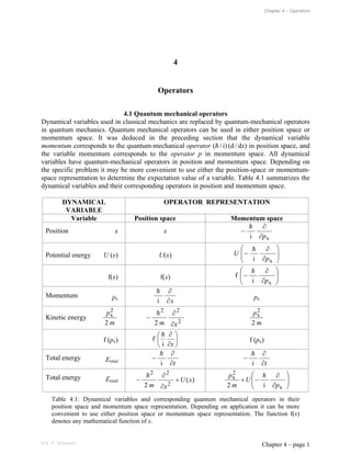
- 1. Chapter 4 – Operators © E. F. Schubert Chapter 4 – page 1 4 Operators 4.1 Quantum mechanical operators Dynamical variables used in classical mechanics are replaced by quantum-mechanical operators in quantum mechanics. Quantum mechanical operators can be used in either position space or momentum space. It was deduced in the preceding section that the dynamical variable momentum corresponds to the quantum-mechanical operator (ƫ / i) (d / dx) in position space, and the variable momentum corresponds to the operator p in momentum space. All dynamical variables have quantum-mechanical operators in position and momentum space. Depending on the specific problem it may be more convenient to use either the position-space or momentum- space representation to determine the expectation value of a variable. Table 4.1 summarizes the dynamical variables and their corresponding operators in position and momentum space. DYNAMICAL VARIABLE OPERATOR REPRESENTATION Variable Position space Momentum space Position x x x i p w w ! Potential energy U (x) U(x) ¸ ¸ ¹ · ¨ ¨ © § w w x i p U ! f(x) f(x) ¸ ¸ ¹ · ¨ ¨ © § w w x i f p ! Momentum px x w w i ! px Kinetic energy m p 2 2 x 2 2 2 2 x m w w ! m p 2 2 x f (px) ¸ ¹ · ¨ © § w w x i f ! f (px) Total energy Etotal t w w i ! t w w i ! Total energy Etotal ) ( 2 2 2 2 x U x m w w ! ¸ ¸ ¹ · ¨ ¨ © § w w x 2 x i 2 p U m p ! Table 4.1: Dynamical variables and corresponding quantum mechanical operators in their position space and momentum space representation. Depending on application it can be more convenient to use either position space or momentum space representation. The function f(x) denotes any mathematical function of x.
- 2. Chapter 4 – Operators © E. F. Schubert Chapter 4 – page 2 Two operator representations for the total energy are given in Table 4.1: The first one, – (ƫ / i) (w / wt), follows from the 4th Postulate. The second one, px 2 / (2 m) + U(x), is the sum of kinetic and potential energy. The specific application determines which of the four operators is most convenient to calculate the total energy. The total energy operator is an important operator. In analogy to the hamiltonian function in classical mechanics, the hamiltonian operator is used in quantum mechanics. The hamiltonian operator thus represents the total energy of the particle represented by the wave function (x) ) ( ) ( ) ( d d 2 ) ( 2 2 2 x x U x x m x H ! (4.1) or equivalently, ) ( ) d d i ( ) ( 2 ) ( 2 p p U p m p p H ) ) ) ! . (4.2) The hamiltonian operator is of great importance because many problems of quantum mechanics are solved by minimizing the total energy of a particle or a system of particles. 4.2 Eigenfunctions and eigenvalues Any mathematical rule which changes one function into some other function is called an operation. Such an operation requires an operator, which provides the mathematical rule for the operation, and an operand which is the initial function that will be changed under the operation. Quantum mechanical operators act on the wave function (x, t). Thus, the wave function (x, t) is the operand. Examples for operators are the differential operator (d / dx) or the integral operator ³ … dx. In the following sections we shall use the symbol [op for an operator and the symbol f(x) for an operand. The definition of the eigenfunction and the eigenvalue of an operator is as follows: If the effect of an operator [op operating on a function f(x) is that the function f(x) is modified only by the multiplication with a scalar, then the function f(x) is called the eigenfunction of the operator [op, that is ) ( f ) ( f s op x x O [ (4.3) where Os is a scalar (constant). Os is called the eigenvalue of the eigenfunction. For example, the eigenfunctions of the differential operator are exponential functions, because x x x s s e e d d s O O O (4.4) where Os is the eigenvalue of the exponential function and the differential operator. 4.3 Linear operators Virtually all operators in quantum mechanics are linear operators. An operator is a linear operator if
- 3. Chapter 4 – Operators © E. F. Schubert Chapter 4 – page 3 ) ( ) ( op op x c x c [ [ (4.5) where c is a constant. For example d / dx is a linear operator, since the constant c can be exchanged with the operator d / dx. On the other hand, the logarithmic operator (log) is not a linear operator, as can be easily verified. In classical mechanics, dynamical variables obey the commutation law. For example, the product of the two variables position and momentum commutes, that is x p p x . (4.6) However, in quantum mechanics the two linear operators, which correspond to x and p, do not commute, as can be easily shown. One obtains ) ( d d i ) ( x x x x p x ¸ ¸ ¹ · ¨ ¨ © § ! (4.7) and alternatively ) ( d d i ) ( i ) ( d d i ) ( x x x x x x x x x p ! ! ! . (4.8) Linear operators do not commute, since the result of Eqs. (4.7) and (4.8) are different. 4.4 Hermitian operators In addition to linearity, most of the operators in quantum mechanics possess a property which is known as hermiticity. Such operators are hermitian operators, which will be defined in this section. The expectation value of a dynamical variable is given by the 5th Postulate according to x x x d ) ( ) ( op * [ [ ³ f f . (4.9) The expectation value ¢[² is now assumed to be a physically observable quantity such as position or momentum. Thus, the dynamical variable [ is real, and [ is identical to its complex conjugate. * * and [ [ [ [ . (4.10) It is important to note that [op z [op*. To determine the complex conjugate form of Eq. (4.9) one has to replace each factor of the integrand with its complex conjugate. x x x d ) ( ) ( * * op * [ [ ³ f f . (4.11) With Eq. (4.10) one obtains x x x x x x d ) ( ) ( d ) ( ) ( * * op op * [ [ ³ ³ f f f f . (4.12) Operators which satisfy Eq. (4.12) are called hermitian operators.
- 4. Chapter 4 – Operators © E. F. Schubert Chapter 4 – page 4 The definition of an hermitian operator is in fact more general than given above. In general, hermitian operators satisfy the condition x x x x x x d ) ( ) ( d ) ( ) ( * 1 * op 2 2 op * 1 [ [ ³ ³ f f f f (4.13) where 1(x) and 2(x) may be different functions. If 1(x) and 2(x) are identical, Eq. (4.13) simplifies into Eq. (4.12). As an example, we consider the observable variable momentum. It is easily shown that the momentum operator is an hermitian operator. The momentum expectation value is given by x x x x p d ) ( d d i ) ( * ³ f f ! . (4.14) Integration by part (recall: x v u v u x v u b a b a b a d d ³ ³ c c ) and using (x o f) = 0 yields x x x x p d ) ( d d i ) ( * ¸ ¸ ¹ · ¨ ¨ © § ³ f f ! (4.15) which proves that p is an hermitian operator. There are a number of consequences and characteristics resulting from the hermiticity of an operator. Two more characteristics of hermitian operators will explicitly mentioned: First, eigenvalues of hermitian operators are real. To prove this, suppose [op is an hermitian operator with eigenfunction (x) and eigenvalue O. Then x x x d ) ( ) ( op * [ ³ f f x x x d ) ( ) ( * O ³ f f (4.16) x x x d ) ( ) ( * O ³ f f (4.17) and also due to hermiticity of the operator x x x d ) ( ) ( * * op [ ³ f f x x x d ) ( ) ( * * O ³ f f (4.18) x x x d ) ( ) ( * * O ³ f f (4.19) Since Eqs. (4.17) and (4.19) are identical, therefore O = O* , which is only true if O is real. Thus, eigenvalues of hermitian operators are real. Second, eigenfunctions corresponding to two unequal eigenvalues of an hermitian operator are orthogonal to each other. This is, if [op is an hermitian operator and 1(x) and 2(x) are eigenfunctions of this operator and O1 and O2 are eigenvalues of this operator then
- 5. Chapter 4 – Operators © E. F. Schubert Chapter 4 – page 5 0 d ) ( ) ( 2 * 1 ³ f f x x x . (4.20) The two eigenfunctions 1(x) and 2(x) are orthogonal if they satisfy Eq. (4.20). The statement can be proven by using the hermiticity of the operator [op. This yields x x x x x x d ) ( ) ( d ) ( ) ( * 1 * op 2 2 op * 1 [ [ ³ ³ f f f f . (4.21) Employing that O1 and O2 are the eigenvalues of 1(x) and 2(x) yields x x x x x x d ) ( ) ( d ) ( ) ( 2 * 1 1 2 * 1 2 O O ³ ³ f f f f . (4.22) Since O1 and O2 are unequal, Eq. (4.22) can only be true if 1(x) and 2(x) are orthogonal functions as defined in Eq. (4.20). 4.5 The Dirac bracket notation A notation which offers the advantage of great convenience was introduced by Dirac (1926). As shown in the proceeding section, wave functions can be represented in position space and, with the identical physical content, in momentum space. Dirac’s notation provides a notation which is independent of the representation, that is, a notation valid for the position-space and momentum- space representation. Let (x, t) be a wave function and let [op be an operator; then the following integration is written with the Dirac bracket notation as x t x t x d ) , ( ) , ( op * op [ [ ³ f f (4.23) and equivalently in momentum space p t p t p d ) , ( ) , ( op * op ) [ ) [ ³ f f . (4.24) It is important to note the following two points. First, because Dirac’s notation is valid for the position- and momentum-space representation, the dependences of the wave function on x, t, or p can be left out. Thus, only and not (x, t) or (p, t) may be used in the Dirac notation. However, if desirable, the explicit dependence of on x, t, or p can be included, for example ¢(x) | [op | (x)². Second, the left-hand-side wave function in the bracket is by definition the complex conjugate of the right-hand-side wave function of the bracket. The integral notation still provides the explicit notation for the complex conjugate wave function, as shown by the asterisk (*). If the operator equals the unit-operator [op = 1, then [ 1 op . (4.25) For convenience the unit operator can be left out
- 6. Chapter 4 – Operators © E. F. Schubert Chapter 4 – page 6 1 1 . (4.26) The normalization condition, given in the 2nd Postulate can then be written as 1 d ) , ( ) , ( * – ³ f f x t x t x . (4.27) The Dirac notation can also be used to express expectation values. Writing the 5th Postulate in the Dirac’s notation, one obtains the expectation value ¢[² of a dynamical variable [, which corresponds to the operator [op, by [ [ op . (4.28) Again, either position-space or momentum space representation of the wave function can be used. In the Dirac notation, the operator acts on the function on the right hand side of the bracket. To visualize this fact one can write 2 op 1 2 op 1 [ [ . (4.29) If it is required that the operator acts on the first, complex conjugate function, the following notation is used x x x d ) ( ) ( * 1 * op 2 – 2 1 op [ [ ³ f f . (4.30) Using this notation, the definition for hermiticity of operators reads 2 1 op 2 op 1 [ [ (4.31) or equivalently * 1 op 2 2 op 1 [ [ . (4.32) This equation is equivalent to the definition of hermitian operators in Eq. (4.13). 4.6 The Dirac delta function A valuable function frequently used in quantum mechanics and other fields is the Dirac delta function. The delta function of the variable x is defined as f G ) ( 0 x x (x = x0) (4.33) 0 ) ( 0 G x x (x z x0) . (4.34) The integral over the delta (G) function remains finite and the integral has the unit value
- 7. Chapter 4 – Operators © E. F. Schubert Chapter 4 – page 7 1 d ) ( 0 – G ³ f f x x x . (4.35) The G function can be understood as the limit of a gaussian distribution with an infinitesimally small standard deviation, that is » » ¼ º « « ¬ ª ¸ ¹ · ¨ © § V S V G o V 2 0 0 0 2 1 exp 2 1 lim ) ( x x x x . (4.36) Gaussian functions with different standard deviations but the same area under the curve are shown in Fig. 4.1. The G function can also be represented by its Fourier integral y x x y x x d e 2 1 ) ( ) ( i – 0 0 f f ³ S G . (4.37) The following equations summarize frequently used properties of the G function ) ( ) ( x x G G (4.38) ) ( 1 ) ( x x G D D G (4.39) ) ( ) ( f ) ( ) ( f 0 0 0 x x x x x x G G (4.40) ) ( f d ) ( ) ( f 0 0 – x x x x x G ³ f f (4.41) 0 ) f( d d d ) ( d d ) ( f 0 – x x x x x x x x x f f G ³ (4.42)
- 8. Chapter 4 – Operators © E. F. Schubert Chapter 4 – page 8 References Dirac P. A. M. “On the theory of quantum mechanics” Proceedings of the Royal Society A109, 642 (1926)
- 9. Chapter 5 – The Heisenberg uncertainty principle © E. F. Schubert Chapter 5 – page 1 5 The Heisenberg uncertainty principle 5.1 Definition of uncertainty Quantum mechanical systems do not allow predictions of their future state with arbitrary accuracy. For example, the outcome of a diffraction experiment such as the Davisson and Germer experiment can be predicted only in terms of a probability distribution. It is impossible to predict or calculate the exact trajectory of an individual quantum mechanical particle. The Heisenberg uncertainty principle (Heisenberg, 1927) allows us to quantify the uncertainty associated with quantum mechanical particles. The uncertainty of a dynamical variable, '[, is defined as
- 11. . 2 2 [ [ [ ' (5.1) Thus, '[ is the mean deviation of a variable [ from its expectation value ¢[². The mean deviation can be understood as the most probable deviation. Using the fact that the expectation value of a sum of variables is identical to the sum of the expectation values of these variables, that is ¦ ¦ [ [ i i i i (5.2) one obtains by squaring out Eq. (5.1)
- 12. . 2 2 2 [ [ [ ' (5.3) Having defined the meaning of uncertainty, we proceed to quantify the uncertainty. 5.2 Position–momentum uncertainty In order to quantify the uncertainty associated with a quantum mechanical system, consider a wave function of gaussian shape as shown in Fig. 5.1. The position space wave function is given by the gaussian function 2 2 1 e 2 ) ( ¸ ¸ ¹ · ¨ ¨ © § V S V x x x x A x . (5.4) The constant Ax is used to normalize the wave function using ¢°² = 1, which yields
- 13. Chapter 5 – The Heisenberg uncertainty principle © E. F. Schubert Chapter 5 – page 2
- 14. x x A V S 4 / 1 4 . (5.5) This wave function may represent a particle localized in a potential well. If the barriers of the well are sufficiently high the particle cannot escape from the well. That is, the wave function is stationary, i. e. (x) does not depend on time. The momentum distribution which corresponds to the gaussian wave function can be obtained by the Fourier integral . d e ) ( 2 1 ) ( / i x x p px ! ! f f S ) ³ (5.6) Inserting the wave function, given by Eq. (5.4), into the Fourier integral yields
- 16. 2 / 2 1 4 / 1 e / 2 1 4 ) ( ¸ ¸ ¹ · ¨ ¨ © § V V S V S ) x p x x p ! ! ! . (5.7) This function represents a gaussian function with a prefactor. Thus, the Fourier transform of a gaussian function is also a gaussian function. The gaussian function in Eq. (5.7) has a standard deviation of ƫ / Vx which has the dimension of momentum. Therefore, we introduce the standard deviation in momentum space x p V V / ! . (5.8) In analogy to Eq. (5.5), we define the normalization constant Ap as
- 17. p p A V S 4 / 1 4 . (5.9) Equation (5.7) can be rewritten using the normalization constant Ap. 2 2 1 e 2 ) ( ¸ ¸ ¹ · ¨ ¨ © § V V S ) p p p p A p . (5.10) This equation is formally identical to the position-space representation of the wave function given by Eq. (5.4). It can be easily verified that the momentum space representation of the state function is normalized as well ¢)(p)°)(p)² = 1. The position and momentum representations of the wave function are shown in Fig. 5.1. The position space and momentum space representation of a gaussian wave function allows us to form the product of the position and momentum uncertainty using Eq. (5.8) ! V V p x . (5.11) Thus, the product of position uncertainty and momentum uncertainty is a constant. Hence a small position uncertainty results in a large momentum uncertainty and vice versa. The uncertainty of the position 'x, as defined by Eq. (5.1) is, in the case of a gaussian function, identical to the
- 18. Chapter 5 – The Heisenberg uncertainty principle © E. F. Schubert Chapter 5 – page 3 standard deviation Vx of that gaussian function. Thus, Eq. (5.11) can be rewritten in its more popular form ! ' ' p x . (5.12) This relation was derived for gaussian wave functions and it applies, in a strict sense, only a gaussian wave functions. If the above calculation is performed for wave functions other than a gaussian (e. g. square-shaped or sinusoidal), then the uncertainty associated with 'x and 'p is larger. Hence, the general formulation of the position–momentum form of the Heisenberg uncertainty relation is given by ! t ' ' p x (5.13) The uncertainty principle shows that an accurate determination of both, position and momentum, cannot be achieved. If a particle is localized on the x axis with a small position uncertainty 'x, then this localization is achieved at the expense of a large momentum uncertainty 'p. 5.3 Energy–time uncertainty The uncertainty relation between position and momentum will now be modified using the group velocity relation, the de Broglie relation, and the Planck relation to obtain a second uncertainty relation between time and energy. The starting point for this modification is a wave packet that propagates with the group velocity Qgr = 'x / 't = 'Z/ 'k. Inserting this relation and the de Broglie relation 'p = ƫ 'k into the position-momentum uncertainty relation of Eq. (5.13) yields 1 t Z ' 't . (5.14) It is now straightforward to obtain a second uncertainty relation by employing the Planck relation 'E = ƫ 'Z, which yields ! t ' ' t E (5.15) which is the energy–time form of the Heisenberg uncertainty relation. This relation states that the energy of a quantum mechanical state can be obtained with highest precision (small 'E), if
- 19. Chapter 5 – The Heisenberg uncertainty principle © E. F. Schubert Chapter 5 – page 4 the uncertainty in time is large, i. e. for long observation times for quantum-mechanical transitions with a long lifetimes. The uncertainty relations are valid between the variables x and p (Eq. 5.13) as well as E and t (Eq. 5.15). These pairs of variables are called canonically conjugated variables. A small uncertainty of one variable implies a large uncertainty of the other variable of the same pair. On the other hand, the two pairs of variables x, p and E, t are independent. For example a large uncertainty in the momentum does not allow any statement about the uncertainty in energy. The uncertainty principle requires that the deterministic nature of classical mechanics be revised. If an uncertainty of momentum or position exists, it is impossible to determine the future trajectory of a particle. On the other hand, the correspondence principle requires that quantum mechanics merges into classical mechanics in the classical limit. Therefore, the uncertainty of 'x or 'p should be insignificantly small in classical physics. Exercise 1: Significance of the uncertainty principle in the macroscopic domain. To see the insignificance of the uncertainty principle in the macroscopic physical world, a body with mass m = 1 kg and velocity v = 1 m / s is considered. The body moves along the x axis and the position of its centroid is assumed to be known to an accuracy of 'x0 = 1 Å. Calculate the position uncertainty after a time of 10 000 seconds. Solution: The initial momentum uncertainty is given by 'p0 | ƫ / 'x0 | 1024 kg m / s. After 10,000 seconds with no forces acting on the body, the position uncertainty is given by 'x = 'x0 + ('p0 / m) t | 1 Å + 10 10 Å . (5.16) This exercise elucidates that the uncertainty principle does not contribute a significant uncertainty in classical mechanics. Thus, even though the trajectory of a macroscopic body cannot be determined in a strict sense, the associated uncertainty is insignificantly small. Even after a time of 1018 s (which is 30 u 109 years, i. e. approximately the age of the universe) the position uncertainty would be just 1 Pm, which is still very small. Exercise 2: The natural linewidth of optical transitions. Consider a quantum mechanical transition from an excited atomic state to a ground state. Assume that the spontaneous emission lifetime of the transition is W. The uncertainty relation gives the spectral width of the emission as 'E = ƫ / W . (5.17) This linewidth is referred to as the natural linewidth of a homogeneously broadened emission line. Problem: Assume that the transition probability follows an exponential distribution, as shown in Fig. 5.2. Calculate the spectral shape of the emission line. What is the natural linewidth of a single quantum transition with lifetime 10 ns? Why is the spectral width of a light-emitting diode (LED), typically 50–100 meV at 300 K, much broader than the natural emission linewidth?