SlideShare a Scribd company logo
1 of 318
Download to read offline
Software, Training & Consulting: Statistics Made Easy® Rev. 5/2/14
Getting started with v9 of Design-Expert software  1
Design-Expert®
Software: WhyVersion 9 is MightyFine!
What’s in it for You
Stat-Ease, Inc. welcomes you to version 9 (v9) of Design-Expert software (DX9) for design of
experiments (DOE). Use this Windows®-based program to optimize your product or process. It
provides many powerful statistical tools, such as:
 Two-level factorial screening designs: Identify the vital factors that affect your process or
product so you can make breakthrough improvements.
 General factorial studies: Discover the best combination of categorical factors, such as
source versus type of raw material supply.
 Response surface methods (RSM): Find the optimal process settings to achieve peak
performance.
 Mixture design techniques: Discover the ideal recipe for your product formulation.
 Combinations of process factors, mixture components, and categorical factors: Mix your
cake (with different ingredients) and bake it too!
Your Design-Expert program offers rotatable 3D plots to easily view response surfaces from all
angles. Use your mouse to set flags and explore the contours on interactive 2D graphs. Our
numerical optimization function finds maximum desirability for dozens of responses
simultaneously!
You’ll find a wealth of statistical details within the program itself via various Help screens. Take
advantage of this information gold-mine that is literally at your fingertips. Also, do not overlook
the helpful annotations provided on all reports.
For a helpful collection of checklists and ‘cheat sheets,’ see the Handbook for Experimenters. It’s
free to all registered users. Furthermore, for quick primers on the principles of design and
analysis, we recommend you read the following two soft-cover books from Stat-Ease Principals
Mark Anderson and Pat Whitcomb —published by Productivity Press of New York city:
 DOE Simplified: Practical Tools for Effective Experimentation,
 RSM Simplified: Optimizing Processes Using Response Surface Methods for Design of
Experiments.
Anderson and Whitcomb have also written a Primer on Mixture Design. It’s posted free for all to
read via the “I’m a Formulator” link on the Stat-Ease home page.
Go to http://www.statease.com/prodbook.html for details and ordering information on the
books listed above.
What’s New
Those of you who’ve used previous versions of Design-Expert software will be impressed with
the many improvements in Version 9. Here are the highlights:
Hard-to-change factors handled via split plots
 Two-level, general and optimal factorial split-plot designs: Make it far easier as a practical
matter to experiment when some factors cannot be easily
randomized.
Software, Training & Consulting: Statistics Made Easy® Rev. 5/2/14
Getting started with v9 of Design-Expert software  2
 Half-normal selection of effects from split-plot experiments with test matrices that are
balanced and orthogonal: The vital effects, both whole-
plot (created for the hard-to-change factors) and sub-
plot (factors that can be run in random order), become
apparent at a glance!
 Effects from split plots assessed via REML* and
Kenward-Roger’s approximate F test: See the familiar
p-values that tell you what’s statistically significant.
*(Restricted maximum likelihood)
 Design resolution provided for two-level factorial split plots: Assess from the start whether
your choice suffices for screening main effects (Res
IV) or characterizing interactions (Res V).
 Power calculated for split plots versus the alternative of complete randomization: See how
accommodation of hard-to-
change factors degrades the
ability to detect certain effects.
 Check designs with restricted randomization for REML/OLS* equivalence: Keep things
simple statistically (KISS) in the ANOVA.
*(Ordinary least squares)
Other new design capabilities
 Definitive screening designs: If you want to cull out the vital few from many numeric process
factors, this fractional three-level DOE choice resolves main effects
clear of any two-factor interactions and squared terms (see screen
shot of correlation matrix—more on that later).
 On the Factorial tab select a simple-sample design for mean-model only: Take advantage of
powerful features in Design-Expert software for data characterization,
diagnostics and graphics—for example with raw outputs from a process
being run at steady-state.
Software, Training & Consulting: Statistics Made Easy® Rev. 5/2/14
Getting started with v9 of Design-Expert software  3
Much-improved capabilities to confirm or verify model predictions
 New Post Analysis Node (at bottom of the handy tree structuring of Design, Analysis and
Optimization) contains Point Prediction, Confirmation and
Coefficients Table reports: Old and new features gathered in logical
place at the end of the natural progression from design through
analysis.
 Entry fields for confirmation data and calculation of mean results: Makes it really easy to see
if follow-up runs fall within the sample-size-adjusted prediction intervals.
 Enter verification runs embedded within blocks as controls or appended to your completed
design: Lend veracity to your ultimate model by
these internal checks.
 Verification points displayed on model graphs and raw residual diagnostics: See how closely
these agree to what’s predicted by your model.
New and more-informative graphics
 Adjustably-tuned LOESS fit line for Graph Columns: Draw a curve through a non-linear set of
points as you see fit.
*(Locally weighted scatterplot smoothing.)
Software, Training & Consulting: Statistics Made Easy® Rev. 5/2/14
Getting started with v9 of Design-Expert software  4
 Color-coded correlation grid for graph columns: Identify at a glance any factors that are not
controlled independently of each other, that is, orthogonally; also
useful for seeing how one response correlates to another.*
*(Data shown in screen shot comes from historical data detailed in RSM
Simplified on NFL sacks versus attributes of defensive linemen.)
 Jump to run added to Factors Tool for model graphs:
For multidimensional experimental regions, find the
slice of interest (containing the point you want to see) at
the press of a button.
 When jumping to a run, the range expands to include the design point: Use this feature to
check how well your model fits—comparing the
actual result versus what is predicted via the
surface graph (in this case very well—the circled
red point is barely beneath the surface!).
 Ignored (and missing) runs can be shown on graphs: Good to be reminded that the original
design called for this, but for one reason or another, you ignored the
outcome (or the response could not be collected, or it was skipped).
 Choice to do diagnostic graphs with externally-studentized residuals (now the default): This
deletion-diagnostic (vs internally-studentized) provides a more sensitive
view of potential abnormalities.
B: Trip (mm)
D: Fast Shot (mm)
390 395 400 405
Defects(Fraction)
0.00
0.20
0.40
0.60
0.80
1.00
D-
D+
Interaction
Software, Training & Consulting: Statistics Made Easy® Rev. 5/2/14
Getting started with v9 of Design-Expert software  5
0.00 5.11 10.22 15.33 20.44
0.0
10.0
20.0
30.0
50.0
70.0
80.0
90.0
95.0
Half-Normal Plot
|Normal Effect|
Half-Normal%Probability
A-Homework
 Many new icons, such as ones for Clear Points and Pop-Out View on the Diagnostics Tool:
Jump to features used frequently more quickly via these handy markers (also they look good!).
 Three-component contour graphs in reals: Get a better view of the restrictions placed on your
mixture space by the constraints you enter on each
component and the total.
 Half-normal plot for one-factor categorical experiments with replicates: See at a glance if
anything significant emerges.
Greater flexibility in data display and export
 Descending sort of all individual design layout columns via right-click menu (shown) or
double-click on header (toggles with ascending sort—previously the
only option): Helpful, for example, when minimum response is desired.
 Identify via “Build Type” the predetermined Model, Lack of Fit, Center, and Replicate points
in your design layout: Dissect the matrix laid out for optimal (I, D, etc) experiments.
 Switch directly between continuous and discrete point type: Sometimes the settings for a
factor cannot be easily changed (for example, diameter of molded
part)—then it pays to recognize them as discrete, thus enabling
the numeric optimizer being set so it will not stray away from
specific values.
 Ignorable block and/or factor columns: Handy for “what-if” analysis, such as what would
have happened if you had not blocked your experiment.
A: Water (%)
5.000
B: Alcohol (%)
4.000
C: Urea (%)
4.000
2.000 2.000
3.000
Viscosity (mPa-sec)
40
60
60
80
80
100
120
2
2 2
2
Software, Training & Consulting: Statistics Made Easy® Rev. 5/2/14
Getting started with v9 of Design-Expert software  6
 Journal feature to export data directly to Microsoft Word or Powerpoint: Fast and formatted
for you to quickly generate a presentable report on your
experimental results.
 Improved copy/paste of Final Equation from the analysis of variance (ANOVA) report to
Microsoft Excel: This not only saves tedious transcription of
coefficients but it also sets up a calculator for you to ‘plug and
chug’, that is, enter into the spreadsheet cells what values for the
inputs you’d like to evaluate and see what the model predicts for
your response.
 From Evaluation and ANOVA screens, the X matrix can be viewed and exported: This is
helpful, for example, for copy and paste to R or Matlab
where statisticians can do further manipulations for
research purposes.
 Display full precision of F-test: If just presenting p<0.0001 is not precise enough, show all the
decimals.
 New XML* script commands for exporting point predictions: Helpful for situations where one
wants to automate the transfer of vital outputs from Design-Expert to other programs.
*(Extensible Markup Language)
More powerful tools for modeling
 Design model included in Fit Summary: This can be very helpful for combined designs such as
response surface optimizations that
include categorical factors (in this case
recommending a model that included
some cross-product terms of 3rd order,
which provided a better fit of the data).
Software, Training & Consulting: Statistics Made Easy® Rev. 5/2/14
Getting started with v9 of Design-Expert software  7
 All-hierarchical model (AHM) selection: Sort through all possible models up to the one you
designed the experiment for, but all the while maintain
hierarchy of terms so you do not end up with something ill-
formulated.
(PS. The alpha out is enforced after AHM is completed by doing a final sweep
using backward selection, after which hierarchy is again corrected by the
program.)
 Non-linear equations involving trigonometric, exponential and other functions allowed for
creating deterministic responses
(for example—costs) or
simulations: This will be
especially helpful for setting up
more realistic scenarios for
students to solve during hands-on
workshops for teaching DOE.
(PS. Simulator now provides an entry field for ratio of variance between whole and sub plots so trainers can set up
split-plot exercises.)
 Special quartic Scheffé polynomial included in automatic selection for mixture modeling:
Sometimes this added degree (4th!) of
non-linear blending helps to better
shape the response surface—making it
better for predictive purposes.
More choices when custom-designing your experiment
 Required model points set aside from optional additional ones that may be needed for
adequate sizing of the design: Prevents setting
up an experiment with too few points to fit the
chosen model.
 Enter a single factor constraint for response surface designs: Creates a ‘hard’ limit on inputs
that cannot go beyond a certain
point (such as zero time) physically
or operationally.
Software, Training & Consulting: Statistics Made Easy® Rev. 5/2/14
Getting started with v9 of Design-Expert software  8
 Greater flexibility in setting up models: For example you can now create an optimal model for
experiment on mixtures with varying categorical ingredients, some of which can go to zero.*
*(See presentation of “Categoric Mixture Components Proportion Going to Zero” by Pat Whitcomb, ENBIS-12,
Ljubljana, Slovenia. Slides available on request to stathelp@statease.com.)
 Save candidate sets in actuals: More flexibility for customizing your experiment design.
More capability for numerical optimization
 Include Cpk* as a goal: Meet quality goals explicitly.
*(A process capability index widely used for Six Sigma and Design
for Six Sigma programs.)
Enhanced design evaluation
 Random model generator provided to generate a realistic response via a quadratic
polynomial with coefficients picked by chance: Use this to play around with how the software
presents the analysis—better than just generating random numbers that only fit a mean
model.
 One-sided option added to FDS* graph: Size your design properly for a verification
experiment done to create a QBD** design space.
*(Fraction of design space)
**(Quality by Design—a protocol promoted by the US Food & Drug
Administration (FDA).)
Many things made nicer, easier, more configurable and faster
 Components that do not vary in a mixture experiment can now be included in the design
build—see them highlighted with gray in the layout:
Provide a recipe sheet that encompasses the entire
formulation, not just what will be manipulated in
your study.
 Automatically re-sort by run order after re-randomizing: A little feature that saves users a
bother.
 Diagnostics report now can be sorted by any of the statistics listed: This enables a more
informative ordering than by run number (the default).
 Faster display of graphs: Great for dazzling your audience with 3D graphs in high resolution.
Software, Training & Consulting: Statistics Made Easy® Rev. 5/2/14
Getting started with v9 of Design-Expert software  9
 Pop-out views numbered: Makes it easier to distinguish and find the associated view-Tool
when re-arranging on your
desktop.
 Graph state stored with file: Restores setting to the way you liked them.
 Improved graphics on Transformation screen: Looks more elegant—better to show off your
results via live presentations or webinars.
 Fonts on analysis tabs now configurable under Edit Preferences (Dialog Control): Go ahead
and make them Comic Sans if you
would like to lighten things up. ; )
Safety net expanded—more mistakes caught and ‘heads-ups’ given
 Warning when largest effect not selected on half-normal plot: This would not make sense, but
it might happen due to, for example, not lassoing
points correctly.
 Hover Help added to select fields: When your mouse goes over an entry place, the program
fills you in with a bit more information on what’s
entailed in the feature you are specifying.
0.00 0.10 0.20 0.30 0.40 0.50
0
10
20
30
50
70
80
90
95
99
Half-Normal Plot
|Standardized Effect|
Half-Normal%Probability
B-Flow
D-Mud
Warning! Largest effect not selected.
Software, Training & Consulting: Statistics Made Easy® Rev. 5/2/14
Getting started with v9 of Design-Expert software  10
Niceties that only statisticians might truly appreciate
 Mean correction for transformation bias when responses displayed in original scale: All you
need to know is that our statisticians figured out how to eliminate a tricky, little-known bias!
 Propagation of error (POE) carried out to the second derivative: Makes POE more accurate.
 Display confidence bands with or without POE added: Easier to match output with other
programs that do not offer POE features like this.
 Add unblocked results to evaluation of blocked experiments: Aids in comparing designs on
the basis of matrix measures.
 Scale to largest estimable effect those normal effects that cannot be otherwise estimated:
This can happen when effects become too large compared to the error estimated by chi-
square.
 Preference now available to display p values to full precision: Previously the program
restricted p values to four decimals, which in some cases did not go far enough.
Technical stuff only those adept at programming will ‘get’
 Automatically generate DTD* files: Now these will always be up to date.
*(Document Type Definition)
 New command to export runs of a specific type: Particularly useful for verification points.
Good news for network administrators
 New more flexible and easier-to-use license manager with greater power to serve
enterprise users: For example, network ‘seats’ can be checked out to individual laptops and
multiple opening of the program on a specific computer will only use one seat.
New Designs and Name Changes in V9 of Design-Expert® Software
There have been many improvements in Design-Expert (DX9) version 9, notably split-plot designs, which
accommodate hard-to-change factors by restricting their randomization into groups. These new designs
can be seen at the bottom of the factorial design builder in DX9 (see the box in the screenshot, below
right). Randomized designs remain available, but some feature new, more descriptive names, and they
have been resorted for easier access. As always in Stat-Ease software, the most commonly used designs
get top priority, that is, they are listed in order of usefulness.
For a quick overview of the changes, compare the screenshots below.
Design-Expert V8 Software – Old Design-Expert V9 Software – New!
New Design
New Designs
Z:ManualDX9DX9-02-1-Simple-Sample-FT.docx5/2/2014 9:18:00 AM
Design-Expert® software version 9: Simple Sample Design
Version 9 of Design-Expert (DX9) features a “simple sample design” that facilitates a straight-forward
analysis of raw data, making it easy to calculate the mean
and other statistics that characterize measurements.
To illustrate the simple sample tools of DX9, let’s
characterize the performance of a motor-shaft supplier.
The data, shown below, is a measure of the endplay:
61, 61, 57, 56, 60, 52, 62, 59, 62, 67, 55, 56, 52, 60, 59, 59,
60, 59, 49, 42, 55, 67, 53, 66, 60. The purchaser needs the
mean, standard deviation, and 95% confidence interval of
this vital attribute.
Off the Factorial tab select Simple Sample and, as shown in
the screen shot, enter the Response Name “Endplay” and
Rows 25 for the number of observations. Then click
Continue. The program then presents a blank data entry
sheet—a “design layout.”
Either type in the data now or open the file “Simple Sample-Motor Shaft.dxpx” that has it pre-entered.
Now proceed with
the analysis by going
to the R1: Endplay
node and pressing
forward to the
ANOVA tab. Design-
Expert then presents
the needed statistics
as seen here.
Check out the graphs
under Diagnostics
(run 20 bears
watching as you will see by changing to the Externally Studentized scale for the Resid vs Run chart) as
well as the 95%-confidence-
banded model graph copied out to
the right. Also, take a look at the
tool under the Post Analysis node
for Point Prediction, in particular
the tolerance interval, a very
useful statistic for a purchaser who
needs to establish incoming
specifications.
This concludes our feature tour of
simple sample tools in DX9. Feel
free to explore other tools. If you
need more information at any
time, press for Tips, Screen Tips off
the main menu or push the light bulb icon.
Design-Expert® Software
Endplay
Design Points
95% CI Bands
Std # 20 Run # 20
Y = Endplay = 42
CI = (55.6418, 60.2782)
Run Number
1 2 3 4 5 6 7 8 9 10 11 12 13 14 15 16 17 18 19 20 21 22 23 24 25
Endplay
40
45
50
55
60
65
70
Simple Sample
DX9-02-2-Gen1Factor.docx Rev. 5/2/14
Design-Expert 9 User’s Guide General One-Factor Multilevel-Categoric Tutorial  1
General Multilevel-Categoric One-Factor
Tutorial
Part 1 – The Basics
Introduction
In this tutorial you will build a general one-factor multilevel-categoric design using
Design-Expert® software. This type of design is very useful for simple comparisons of
categorical treatments, such as:
 Who will be the best supplier,
 Which type of raw material should be selected,
 What happens when you change procedures for processing paperwork.
If you are in a hurry, skip the boxed bits—these are sidebars for those who want to spend
more time and explore things.
 Explore response surface methods: If you wish to experiment on a continuous factor, such as time, which can be
adjusted to any numerical level, consider using response surface methods (RSM) instead. This is covered in a series of
tutorials presented later in the Design-Expert User’s Guide.
The data for this example come from the Stat-Ease bowling league. Three bowlers (Pat,
Mark, and Shari) are competing for the last team position. They each bowl six games in
random order – ideal for proper experimentation protocol. Results are:
Game Pat Mark Shari
1 160 165 166
2 150 180 158
3 140 170 145
4 167 185 161
5 157 195 151
6 148 175 156
Mean 153.7 178.3 156.2
Bowling scores
Being a good experimenter, the team captain knows better than to simply pick the bowler
with the highest mean score. The captain needs to know if the average scores are
significantly different, given the variability in individual games. Maybe it’s a fluke that
Mark’s score is highest.
This one-factor case study provides a good introduction to the power of simple comparative
design of experiments (DOE). It exercises many handy features found in Design-Expert
software.
 Explore other resources: We won’t explain all features displayed in this current exercise because most will be
covered in later tutorials. Many other features and outputs are detailed only in the help system, which you can access by
clicking Help in the main menu, or in most places via a right click, or by pressing the F1 key (context sensitive).
2  General Multilevel-Categoric One-Factor Tutorial Design-Expert 9 User’s Guide
Design the Experiment
We will assume that you are familiar with your computer’s graphical user interface and
your mouse. Start the program by double clicking the Design-Expert icon. You will then see
the main menu and icon bar.
Click on File in the main menu. Unavailable items are dimmed. (If you prefer using your
keyboard, press the Alt key and underlined letter simultaneously, in this case Alt F.)
File menu
Select the New Design item with your mouse.
 Explore optional ways to select a new design: The blank-sheet icon  on the left of the toolbar is a quicker path to
this screen. To try this, press Cancel to re-activate the tool bar.
Opening a new design with the blank sheet icon
Using either path, you now see four yellow tabs on the left of your screen. The Factorial
tab comes up by default. Select Multilevel Categoric for this design. (If your factor is
numerical, such as temperature, then you would use the One Factor option under the
Response Surface tab.)
 Explore what the program tells you in its annotations: Note the helpful description: “Design, also known as
“General Factorial”, for 1 to 12 factors where each factor may have a different number of levels.”
P.S. If any of your factors are quite hard to control, that is, not easily run at random levels, then consider using the Split-
Plot Multilevel Categoric design. However, restricting randomization creates big repercussion on the power of your
experiment, so do your best to allow all factors to vary run-by-run as chance dictates. (Design-Expert by default will lay
out your design in a randomized run order.)
DX9-02-2-Gen1Factor.docx Rev. 5/2/14
Design-Expert 9 User’s Guide General One-Factor Multilevel-Categoric Tutorial  3
Multilevel Categoric design
Enter the Design Parameters
Leave the number of factors at its default level of 1 but click the entry format Vertical
(easier than Horizontal for multiple levels). Enter Bowler as the name of the factor. Tab
down to the Units field and enter Person. Next tab to Type. Leaving Type at its default of
Nominal, tab down to the Levels field and enter 3. Now tab to L(1) (level one) and enter
Pat. Type Mark, and Shari for the other two levels (L2 and L3).
Multilevel Categoric design-builder dialog box – completed
 Explore screen tips: For details on the options for factor type, click the light bulb icon ( ) in the toolbar to access our
context-sensitive screen tips.
Screen tips on factor Type
Press Continue to specify the remaining design options. In the Replicates field, which
becomes active by default, type 6 (each bowler rolls six games). Tab to the “Assign one
block per replicate” field but leave it unchecked. Design-Expert now recalculates the
number of runs for this experiment: 18.
4  General Multilevel-Categoric One-Factor Tutorial Design-Expert 9 User’s Guide
Design options entered
Press Continue. Let’s do the easy things first. Leave the number of Responses at the
default of 1. Now click on the Name box and enter Score. Tab to the Units field and enter
Pins.
Response name dialog box – completed
At this stage you can skip the remainder of the fields and continue on. However, it is good
to gain an assessment of the power of your planned experiment. In this case, as shown in
the fields below, enter the value 20 because the bowling captain does not care if averages
differ by fewer than 20 pins. Then enter the value 10 for standard deviation (derived from
league records as the variability of a typical bowler). Design-Expert then compute a signal-
to-noise ratio of 2 (10 divided by 5).
Optional power calculator – necessary inputs entered
Press Continue to view the happy outcome – power that exceeds 80 percent probability of
seeing the desired difference.
Results of power calculation
Click on Finish for Design-Expert to create the design and take you to the design layout
window.
DX9-02-2-Gen1Factor.docx Rev. 5/2/14
Design-Expert 9 User’s Guide General One-Factor Multilevel-Categoric Tutorial  5
 Explore the program interface: Before moving on, take a look at the unique branching interface provided by Design-
Expert for the design and analysis of experiments and resulting optimization.
Design-Expert software’s easy-to-use branching interface
You will explore some branches in this series of tutorials and others if you progress to more advanced features, such as
response surface methods for process optimization.
Save the Design
When you complete the design setup, save it to a file by selecting File, Save As. Type in the
name of your choice (for this tutorial, we suggest Bowling) for your data file, which is
saved as a *.dxpx type.
Save As dialog box
Click on Save. Now you’re protected in case of a system crash.
Create a Data Entry Form
In the floating Design Tool click Run Sheet (or go to the View menu and select Run Sheet)
to produce a recipe sheet for your experiment with your runs in randomized order. A
printout provides space to write down the responses. (Note: this view of the data does not
6  General Multilevel-Categoric One-Factor Tutorial Design-Expert 9 User’s Guide
allow response entry. To type results into the program you must switch back to the home
base – the Design Layout view.)
Run Sheet view (your run order may differ)
 Explore printing features: It’s not necessary for this tutorial, but if you have a printer connected, you can select File,
Print, and OK (or click the printer icon) to make a hard copy. (You can do the same from the basic design layout if you
like that format better.)
Enter the Response Data
When performing your own experiments, you will need to go out and collect the data.
Simulate this by clicking File, Exit. Click on Yes if you are prompted to Save. Now re-start
Design-Expert and use File, Open Design or click the open file icon on the toolbar)) to
open your data file (Bowling.dxpx). You should now see your data tabulated in the
randomized layout. For this example, you must enter your data in the proper order to
match the correct bowlers. To do this, right-click the Factor 1 (A: Bowler) column header
and choose Sort Ascending.
Sort runs by standard (std) order
Now enter the responses from the table on page one, or use the following screen. Except for
run order, your design layout window must look like that shown below.
DX9-02-2-Gen1Factor.docx Rev. 5/2/14
Design-Expert 9 User’s Guide General One-Factor Multilevel-Categoric Tutorial  7
Design Layout in standard order with response data entered
When you conduct your own experiment, be sure to do the runs and enter the response(s)
in randomized order. Standard order should only be used as a convenience for entering
pre-existing design data.
 Explore advantages of being accurate on the actual run order: If you are a real stickler, replace (type over) your run
numbers with the ones shown above, thus preserving the actual bowlers’ game sequence. Bowling six games is taxing
but manageable for any serious bowler. However, short and random breaks while bowling six games protects against
time-related effects such as learning curve (getting better as you go) and/or fatigue (tiring over time).
Save your data by selecting File, Save from the menu (or via the save icon  on the
toolbar). Now you’re backed up in case you mess up your data. This backup is good
because now we’ll demonstrate many beneficial procedures Design-Expert features in its
design layout.
For example, right click the Select button. This allows you to control what
Design-Expert displays. For this exercise, choose Comments.
8  General Multilevel-Categoric One-Factor Tutorial Design-Expert 9 User’s Guide
Select button for choosing what you wish to display in the design layout
In the comments column above we added a notation that after run 8, the bowling alley
proprietor re-oiled the lane – for what that was worth. Seeing Pat’s scores, the effect
evidently was negligible. ; )
 Explore entering comments: Try this if you like. If comments exceed allotted space, move the cursor to the right
border of the column header until it turns into a double-headed arrow (shown below). Then, just double-click for
automatic column re-sizing.
Adjusting column size
Now, to better grasp the bowling results, order them from low-to-high as shown below by
right-clicking the Response column header and selecting Sort Ascending.
Sorting a response column (also works in the factor column)
You’ll find sorting a very useful feature. It works on factors as well as responses. In this
example, you quickly see that Mark bowled almost all the highest games.
DX9-02-2-Gen1Factor.docx Rev. 5/2/14
Design-Expert 9 User’s Guide General One-Factor Multilevel-Categoric Tutorial  9
Analyze the Results
Now we’ll begin data analysis. Under the Analysis branch of the program (on the left side
of your screen), click the Score node. Transform options appear in the main window of
Design-Expert on a progressive tool bar. You’ll click these buttons from left to right and
perform the complete analysis. It’s a very easy process. The Transform screen gives you
the opportunity to select a transformation for the response. This may improve the analysis’
statistical properties.
Transformation button – the starting point for the statistical analysis
 Explore details on transformations: If you need some background on transformations, first try Tips. For complete
details, go to the Help command on the main menu. Click the Search tab and enter “transformations.”
As shown at the bottom of the Transform screen above, the program provides data-
sensitive advice, so press ahead with the default of None by clicking the Effects tab.
Examine the Analysis
By necessity, the tutorial now turns a bit statistical. If this becomes intimidating, we
recommend you attend a basic class on regression, or better yet, a DOE workshop such as
Stat-Ease’s computer-intensive Experiment Design Made Easy.
Design-Expert now pops up a very specialized plot that highlights factor A—the bowlers—
as an emergent effect relative to the statistical error, that is, normal variation, shown by the
line of green triangles.
10  General Multilevel-Categoric One-Factor Tutorial Design-Expert 9 User’s Guide
Initial view of the effect of Bowler
That is good! It supports what was obvious from the raw results—who bowls does matter.
 Explore half-normal plots: If you want to learn more about half-normal plots of effects, work through the Two-Level
Factorial Tutorial.
To get the statistical details, press the ANOVA (Analysis of Variance) tab. Notice to the far
right side of your screen that Design-Expert verifies that the results are significant.
ANOVA results (annotated), with context-sensitive Help enabled via right-click menu
 Explore the ANOVA report: Now select View, Annotated ANOVA from the menu atop the screen and uncheck ()
this option. Note that the blue textual hints and explanations disappear so you can make a clean printout for statistically
savvy clients. Re-select View, Annotated ANOVA to ‘toggle’ back all the helpful hints. Before moving on, try the first
hint shown in blue: “Use your mouse to right click on individual cells for definitions.” For example, perform this tip on
the p-value of 0.0006 as shown above (select Help at the bottom of the pop-up menu). There’s a wealth of information
to be brought up from within the program with a few simple keystrokes: Take advantage!
DX9-02-2-Gen1Factor.docx Rev. 5/2/14
Design-Expert 9 User’s Guide General One-Factor Multilevel-Categoric Tutorial  11
Now click the ‘floating’ (moveable) R-squared Bookmark button (or press the scroll-down
arrow at the bottom right screen) to see various summary statistics.
Summary statistics
 Explore the post-ANOVA statistics: The annotations reveal the gist of what you need to know, but don’t be shy about
clicking on a value and getting online Help via a right-click (or try the F1 key). In most cases you will access helpful
advice about the particular statistic.
Now click the Coefficients Bookmark button to view the output illustrated below.
Coefficient estimates
Here you see statistical details such as coefficient estimates for each model terms and their
confidence intervals (“CI”). The intercept in this simple one-factor comparative experiment
is simply the overall mean score of the three bowlers. You may wonder why only two
terms, A1 and A2, are provided for a predictive model on three bowlers. It turns out that
the last model term, A3, is superfluous because it can be inferred once you know the mean
plus the averages of the other two bowlers.
Now let’s move on to the next section within this screen: “Treatment Means.”
Treatment means
Here are the averages for each of the three bowlers. As you can see below, these are
compared via pair-wise t-tests in the following part of the ANOVA report.
12  General Multilevel-Categoric One-Factor Tutorial Design-Expert 9 User’s Guide
Treatment means
You can conclude from the treatment comparisons that:
 Pat differs significantly (24.67 pins worse!) when compared with Mark (1 vs 2)
 The 2.5 pins mean difference between Pat and Shari (1 vs 3) is not significant (nor
is it considered important by the bowling team’s captain – recall in the design
specification for power that a 10-pin difference was the minimum of interest)
 Mark differs significantly (22.17 pins better!) when compared with Shari (2 vs 3).
 Explore the Top feature: Before moving ahead, press Top on the floating Bookmark. This is a very handy way of
moving through long reports, so it’s worth getting in the habit of using it.
Back to the top
Analyze Residuals
Click the Diagnostics tab to bring up the normal plot of residuals. Ideally this will be a
straight line, indicating no outlying abnormalities.
 Explore the ‘pencil test’: If you have a pencil handy (or anything straight), hold it up to the graph. Does it loosely
cover up all the points? The answer is “Yes” in this example – it passes the “pencil test” for normality. You can
reposition the thin red line by dragging it (place the mouse pointer on the line, hold down the left button, and move the
mouse) or its “pivot point” (the round circle in the middle). However, we don’t recommend you bother doing this – the
program generally places the line in the ideal location automatically. If you need to re-set the line, simply double-click
your left mouse button over the graph.
Notice that the points are coded by color to the level of response they represent – going
from cool blue for lowest values to hot red for the highest. In this example, the red point is
Mark’s outstanding 195 game. Pat and Shari think Mark’s 195 game should be thrown out
because it’s too high. Is this fair? Click this point so it will be highlighted on this and all the
other residual graphs available via the Diagnostics Tool (the ‘floating’ palette on your
screen).
DX9-02-2-Gen1Factor.docx Rev. 5/2/14
Design-Expert 9 User’s Guide General One-Factor Multilevel-Categoric Tutorial  13
Normal probability plot of residuals (195 game highlighted)
 Explore the Top feature: Notice on the Diagnostics Tool that they are “studentized” by default. This converts raw
residuals, reported in original units (‘pins’ of bowling in this example), to dimensionless numbers based on standard
deviations, which come out in plus or minus scale. More details on studentization reside in Help. Raw residuals can be
displayed by choosing it off the down-list on the Diagnostics Tool shown below. Check it out!
Other ways to display residuals
In any case, when runs have greater leverage (another statistical term to look up in Help), only the Studentized form of
residuals produces valid diagnostic graphs. For example, if Pat and Shari succeed in getting Mark’s high game thrown
out (don’t worry – they won’t!), then each of Mark’s remaining five games will exhibit a leverage of 0.2 (1/5) versus
0.167 (1/6) for each of the others’ six games. Due to potential imbalances of this sort, we advise that you always leave
the Studentized feature checked (as done by default). So if you are on Residuals now, go back to the original choice that
came up by default (externally* studentized).
*P.S. Another aspect of how Design-Expert displays residuals by default is them being done “externally”. This is
explored in the Two-Level Factorial Tutorial. For now, suffice it to say that the program chooses this form of residual to
provide greater sensitivity to statistical outliers. This makes it even more compelling not to throw out Mark’s high game.
On the Diagnostics Tool, select Resid. vs. Pred. to generate a plot of residuals for each
individual game versus what is predicted by the response model.
 Explore an apocryphal story: Supposedly, “residuals” were originally termed “error” by statisticians, but the
management people got upset at so many mistakes being made!
Let’s make it easier to see which residual goes with which bowler by pressing the down-list
arrow for the Color by option in the Diagnostics Tool and selecting A:Bowler.
14  General Multilevel-Categoric One-Factor Tutorial Design-Expert 9 User’s Guide
Residuals versus predicted values, colored by bowler
The size of the studentized residual should be independent of its predicted value. In other
words, the vertical spread of the studentized residuals should be approximately the same
for each bowler. In this case the plot looks OK. Don’t be alarmed that Mark’s games stand
out as a whole. The spread from bottom-to-top is not out of line with his competitors,
despite their protestations about the highest score (still highlighted).
Bring up the next graph on the Diagnostics Tool list – Resid. vs Run (residuals versus run
number). (Note: your graph may differ due to randomization.)
Residuals versus run chart (Note: your graph may differ due to randomization)
Here you might see trends due to changing alley conditions (the lane re-oiling, for example),
bowler fatigue, or other time-related lurking variables.
 Explore repercussion of possible trends: In this example things look relatively normal. However, even if you see a
pronounced upward, downward, or shift change, it will probably not bias the outcome because the runs are completely
randomized. To ensure against your experiment being sabotaged by uncontrolled variables, always randomize!
More importantly in this case, all points fall within the limits (calculated at the 95 percent
confidence level). In other words, Mark’s high game does not exhibit anything more than
common-cause variability, so it should not be disqualified.
Design-Expert® Software
Score
Color points by level of
Bowler:
Pat
Mark
Shari
Std # 11 Run # 14
X: 14
Y: 2.175
Run Number
ExternallyStudentizedResiduals
Residuals vs. Run
-4.00
-2.00
0.00
2.00
4.00
1 3 5 7 9 11 13 15 17
DX9-02-2-Gen1Factor.docx Rev. 5/2/14
Design-Expert 9 User’s Guide General One-Factor Multilevel-Categoric Tutorial  15
View the Means and Data Plot
Select the Model Graphs tab from the progressive tool bar to display a plot containing all
the response data and the average value at each level of the treatment (factor). This plot
gives an excellent overview of the data and the effect of the factor levels on the mean and
spread of the response. Note how conveniently Design-Expert scaled the Y axis from 140 to
200 pins in increments of 10.
One-factor effects graph with Mark’s predicted score (mean) highlighted
The squares in this effects plot represent predicted responses for each factor level (bowler).
Click the square representing Mark’s mean score as shown above. Notice that Design-
Expert displays the prediction for this treatment level (reverting to DOE jargon) on the
legend at the left of the graph. Vertical ‘I-beam-shaped’ bars represent the 95% least
significant difference (LSD) intervals for each treatment. Mark’s LSD bars don’t overlap
horizontally with Pat’s or Shari’s, so with at least 95% confidence, Mark’s mean is
significantly higher than the means of the other two bowlers.
 Explore other points on the model graph: Oh, by the way, maybe you noticed that the numerical value for the height
of the LSD bar appeared when you clicked Mark’s square. You can also click on any round point to see the actual
scores. Check it out!
Pat and Shari’s LSD bars overlap horizontally, so we can’t say which of them bowls better. It
seems they must spend a year in a minor bowling league and see if a year’s worth of games
reveals a significant difference in ability. Meanwhile, Mark will be trying to live up to the
high average he exhibited in the tryouts and thus justify being chosen for the Stat-Ease
bowling team.
That’s it for now. Save your results by going to File, Save. You can now Exit
Design-Expert if you like, or keep it open and go on to the next tutorial – part two for
general one-factor design and analysis. It delves into advanced features via further
adventures in bowling.
16  General Multilevel-Categoric One-Factor Tutorial Design-Expert 9 User’s Guide
General One-Factor Tutorial
(Part 2 – Advanced Features)
Digging Deeper Into Diagnostics
(Caution: Only the more daring new users should press ahead from here—those who like to
turn over every rock to see what’s underneath, that is—the types who are curious to know
everything there is to know. If that’s not you, skip the rest and go on to another tutorial if it
offers feature you need for your particular experiment.)
If your bowling data is active in Design-Expert® software from Part 1 of this tutorial,
continue on. If you exited the program, re-start it and use File, Open Design to open data
file (Bowling.dxpx). Otherwise, set up this data file as instructed above in our General
One-Factor Tutorial (Part 1 – The Basics). Then, under the Analysis branch (you may
already be here) click the Score node and press the Diagnostics tab.
We’re now going to look at a new graph in the Diagnostics Tool. Click the Influence
option on the Diagnostics Tool palette. Then click on DFFITS. This statistic, which stands
for difference in fits, measures the change in each predicted value that occurs when that
response is deleted. The larger the absolute value of DFFITS, the more it influences the
fitted model. (For more details on this statistic and the related deletion diagnostic,
DFBETAS, see our program Help or refer to Raymond Myers’ Classical and Modern
Regression with Applications, 2nd Edition (PWS Pub. Co., 1990).)
DFFITS graph (your graph may differ due to random runs)
Notice that one point lies above the rest. (The pattern on your graph may differ from what
we show here due to randomized run order, but this isn’t a concern in this discussion.) The
top-most point is Mark’s high game, which earlier created controversy, particularly among
competitors Pat and Shari. Mark’s point falls far below a relatively conservative high
benchmark of plus-or-minus two for the DFFITS. So, taking all other diagnostics into
consideration, we don’t advise that this particular run be investigated further.
DX9-02-2-Gen1Factor.docx Rev. 5/2/14
Design-Expert 9 User’s Guide General One-Factor Multilevel-Categoric Tutorial  17
Nevertheless, for purposes of learning how to use new Design-Expert software features,
right-click Mark’s top point with your mouse and select Highlight Point as shown below.
Highlighting a point
Myers demonstrates mathematically that the DFFITS statistic is really the externally
studentized residual multiplied by high leverage points. Click the Leverage button and
you’ll see that all runs exhibit equal leverage here because an equal number of runs were
made at each treatment level (all three bowlers rolled six games each).
Leverages
Therefore, this DFFITS exhibits a pattern identical to that shown on the externally
studentized residual graph, which you studied in the preceding tutorial. The reason we’re
reviewing this is to set the stage for what you’ll do later in this tutorial – unbalance the
leverages to make this session more significant for diagnostic purposes.
 Explore the Pop-Out View feature: Now is a good time to go back to the DFFITS plot and press the Pop-Out View
button the very bottom of the Diagnostics Tool.
Pop-Out View button
Next go back via the Diagnostics button to the Resid. vs Run plot and verify the statement above that in this case these
two plots (DFFITs and residuals versus run) exhibit the same pattern. (You may need to press Alt-Tab to get the
windows you want on the same screen.)
18  General Multilevel-Categoric One-Factor Tutorial Design-Expert 9 User’s Guide
Demonstration of pop-out view to see two plots side by side
You’d best now close out the pop-out view by pressing the X at the upper right corner. Otherwise your screen will get
too messy.
Here’s one final Design-Expert software feature for you before we leave the Diagnostics
Tool: Click the Report button to get a table of statistics case-by-case in standard order for
the entire experiment. For those of you who prefer numbers over pictures (statisticians for
sure!), this should satisfy your appetite. Notice that Mark’s high 195 game is highlighted in
blue text as shown below.
Report with case statistics used for preceding diagnostics graphs
Remember, you can right-click any value in reports of this nature within
Design-Expert software to view context-sensitive Help with statistical details.
Modifying the Design Layout
Design-Expert offers great flexibility when modifying data in its design layout. We’ll see in
this bowling scenario how our software allows you to modify an existing design with added
blocks and factor levels.
The outcome of the bowling match appears to be definitive, especially from Mark’s
perspective. But Pat and Shari demand one more chance to prove themselves worthy of the
DX9-02-2-Gen1Factor.docx Rev. 5/2/14
Design-Expert 9 User’s Guide General One-Factor Multilevel-Categoric Tutorial  19
team. They still think Mark’s high 195 game was a fluke, even though this isn’t supported
by the diagnostic analysis. Mark objects and a dispute ensues.
Attempting compromise, the team captain decides to toss out the highest and lowest games
for each of the three bowlers and replace them with two new scores each. But Ben, a newly
hired programmer and avid bowler, arrives at the alley and is allowed to participate in this
second block of runs. (Yes, this makes little sense, but it will add some interest to this tour
of Design-Expert’s flexibility for design and analysis of experiments – no matter how
convoluted they become in actuality.)
It quickly becomes apparent that this new kid does things differently. He’s a lefty with a
huge hook that’s hard to control. To aggravate this variability, Ben does
something very different from other bowlers – he does not put his thumb in
the ball’s hole made for that purpose. When Ben’s odd approach works, the
pins go flying. But as likely as not, that ball slides off into the left gutter or
careens over the edge on the right.
The results for Ben and the three original bowling team candidates are below.
Block Game Pat Mark Shari Ben
1 1 160 165 166 NA
1 2 150 180 158 NA
1 3 140 170 145 NA
1 4 167 185 161 NA
1 5 157 195 151 NA
1 6 148 175 156 NA
2 1 162 175 163 200
2 2 153 180 166 130
Bowling scores with high and low games replaced by two new games (plus a new guy)
To enter this new data (and ignore some of the old), click the Design node near the upper
left of your screen. You should now see the bowling data from the first tutorial. Mark’s high
195 game remains highlighted in blue text (assuming you clicked on it as instructed on page
2 of this tutorial while performing the diagnostics).
Right click the Select column header and click Block. This design attribute is now needed
to accommodate the new bowler’s (Ben’s) incoming score data.
20  General Multilevel-Categoric One-Factor Tutorial Design-Expert 9 User’s Guide
Selecting block to display it as a column in the design layout
Right click the Response column header and choose Sort Ascending. You did this before
in Part 1 so you now have this feature mastered…we hope. ; )
Mark’s best game now drops to the very bottom. Let’s single him out first to placate Pat and
Shari. Right-click the square button at the left of the last row (Mark’s 195 score). Click Set
Row Status, then Ignore as shown below.
Ignoring Mark’s high game
By the way, it’s OK to change your mind when modifying your design layout: You can ‘un-
ignore’ a row by clicking Set Row Status, Normal.
Now let’s really get Pat’s and Shari’s hopes high by excluding their low games from
consideration. Click the square button (in the Select column) to the left of the top row (Pat’s
low 140 game) and, while pressing down the Shift key, also click the button in the Select
column’s second row (Shari’s low 145 game). Release the Shift key. Keep your mouse
within the Select column’s first or second row, right-click and choose Set Row Status,
Ignore for these two low games, as shown below.
DX9-02-2-Gen1Factor.docx Rev. 5/2/14
Design-Expert 9 User’s Guide General One-Factor Multilevel-Categoric Tutorial  21
Ignoring the low games for Pat and Shari
Now move down a few rows and click the square button in the Select column’s row showing
Mark’s low 165 game.
Notice the two rows below Mark’s low 165 game – the high games for Shari (166) and Pat
(167). It’s now time for Shari and Pat to pay the price for complaining. While first pressing
and holding down the Shift key, click the following two square buttons in the Select
column’s row: Shari’s high 166 game and Pat’s high 167 game. Release the Shift key. Three
rows should now be highlighted in light blue as shown below. Keep your mouse within the
Select column’s highlighted three rows, right-click and choose Set Row Status, Ignore.
Ignoring Mark’s low game and the high games for Shari and Pat
Now let’s restore the original layout order. Right-click the Factor 1 (A: Bowler) column
header, then choose Sort Ascending. Compare your screen with what we show below. If
there are differences, fix them now to match this screenshot. However, remember that the
run number is random, so you don’t need to fix that.
22  General Multilevel-Categoric One-Factor Tutorial Design-Expert 9 User’s Guide
Back to standard order after low and high games ignored for each bowler
Now create a new block (needed for the second round of bowling) by right-clicking the
Block column header and choosing Edit Info as shown below.
Creating a new block
You’ll see a form allowing you to assign names to the block(s). Don’t bother doing this now.
As shown below, change Number of Blocks at the top to 2. Press the Tab key to see the
change take effect. (If the name field truncates, click and move the right border of the
column header to re-size it.)
DX9-02-2-Gen1Factor.docx Rev. 5/2/14
Design-Expert 9 User’s Guide General One-Factor Multilevel-Categoric Tutorial  23
Adding a second block of runs
Click OK. It seems that nothing changed, but actually the program now knows that you will
be conducting another block of runs.
Now you are ready to begin adding and/or duplicating rows. This can be accomplished in
different ways, depending on your ingenuity. We’ll follow routes revealing as many of the
editing features as possible, although they may not demonstrate the most elegant
approaches. As shown below, right click the Select column’s square button at the left of the
first row (Pat’s 160 game) to bring up the editing menu. Click the first selection, Insert
Row.
Inserting a new row
You now see a new row containing blanks for the bowler and the score. (Don’t worry if it’s
being ignored – crossed out, that is – for the moment.) Click the first row’s block cell
directly below the block field header, then click the list arrow. Select Block 2 as shown
below.
Changing the block number
Click the blank field for bowler and press the list arrow (). Select Pat. (We’re using
categorical factors here, but if this were a numerical field, you’d enter a value.)
24  General Multilevel-Categoric One-Factor Tutorial Design-Expert 9 User’s Guide
Entering a categorical value for factor
Again, right-click the Select column’s square button at the left of the first row to bring up the
editing menu as shown below. Click Duplicate.
Duplicating a row
Design-Expert may pop up a warning like the one shown below.
Warning about categoric contrasts
The program is recognizing a potential problem here and is alerting you that only one
bowler is in the second block. You need not worry at this stage because you will be adding
others. Click the check option Do not show this warning again. This will save you
aggravation later. Don’t worry – you will not be unprotected indefinitely. This warning will
be re-enabled the next time you start the program.
Turning off a warning (it will come back the next time you run the program)
Press OK to proceed.
Right-click the Block column header and choose Sort Ascending.
Two new rows are now seen at the bottom of your design layout. We need two new rows
apiece for Shari and Mark. Let’s simply duplicate Pat’s two new rows and update the
names. Do this by first clicking the Select column’s square button at the left of Pat’s first
new row, so it is highlighted. Then while holding down the Shift key, click the Select
column’s square button at the left of Pat’s second new row. Both rows should now be
highlighted. (This is a bit tricky, but it saves time.)
DX9-02-2-Gen1Factor.docx Rev. 5/2/14
Design-Expert 9 User’s Guide General One-Factor Multilevel-Categoric Tutorial  25
Now right-click any Select column’s square button at the left of the highlighted block and
select Duplicate. (If the warning screen pops up again, click OK.)
Duplicating a block of rows
In the first duplicated row, click the field for Bowler and select Mark.
Changing name of bowler
Do the same for the last row. You now should have two new rows for both Pat and Mark.
Click the Select column’s square button at the left of Mark’s first new row, so it is
highlighted. Then while holding down the Shift key, click the Select column’s square button
at the left of Mark’s second new row. Both rows should now be highlighted. As before,
right-click any Select column’s square button at the left of the highlighted block and select
Duplicate.
Duplicating two more rows
In the first duplicated row, click the field for Bowler and select Shari. Do the same for the
last row.
26  General Multilevel-Categoric One-Factor Tutorial Design-Expert 9 User’s Guide
Completing lineup for block 2 – the second round of bowling
But what about the new kid – Ben? We need to identify him as a new competitor in this
bowling contest. Do this by right-clicking the header for Bowler and selecting Edit Info.
Getting ready to add a new level for the factor
Change Number of Levels to 4 (see below left).
Adding another bowler
Press Tab once. Click the field intersecting at Name column and row 4 (below right). Type
the name Ben.
Entering the new bowler
Press OK. Now duplicate two more rows by clicking the Select column’s square button at
the left of the first of Shari’s two new games at the bottom of the list. While holding down
the Shift key, click the Select column’s square button at the left of the last run. Finally,
right-click any Select column’s square button at the left of the highlighted block and select
Duplicate.
In both of these new duplicated rows, click the fields for Bowler and select Ben.
DX9-02-2-Gen1Factor.docx Rev. 5/2/14
Design-Expert 9 User’s Guide General One-Factor Multilevel-Categoric Tutorial  27
Ben now on the list as a bowler
An important aside: Always randomize your run orders for actual experiments. For
purposes of this tutorial, this will just be a bother, so do this only if you wish to try it out,
but it’s very easy to do – simply right-click the Run column-header and do this for Block 2
as shown.
How to randomize the run order in the second block
To make it easier to enter the results, right-click the Factor 1 (A: Bowler) column header
and Sort Ascending. Then right-click the Block column header and Sort Ascending.
Now enter the eight new scores as shown below.
Data entered for second block of games
Go ahead now and re-analyze your data by clicking the Score node under Analysis. Move
through Transform and click on the Effects tab. A warning pops up that the design is not
“orthogonal.”
28  General Multilevel-Categoric One-Factor Tutorial Design-Expert 9 User’s Guide
Warning about design now being non-orthogonal
This is a mathematical artifact of our ad hoc addition of runs in a second block. It will not
create any material impact on the outcome so just press on via OK and click the square
appearing at the end of the green triangles (error estimates) on the half-normal plot of
effects. This puts A-Bowler in your model.
Bowler picked on half-normal plot of effects
Proceed to ANOVA (overlooking this model being not significant) and then to
Diagnostics. As you will see, something is abnormal about this data. Do you notice that
the residuals now line up very poorly, especially at the extreme points as shown below? On
the floating Diagnostics Tool change Color by to A: Bowler.
DX9-02-2-Gen1Factor.docx Rev. 5/2/14
Design-Expert 9 User’s Guide General One-Factor Multilevel-Categoric Tutorial  29
Diagnostics for bowling results – part two: Normal plot with poorly aligned residuals
Now (referring to the color key at the left of the plot) you see that the results from Ben do
not fit with the others (his games are the two outliers – low and high). Considering his odd,
unstable style of bowling, this should be no surprise. Click the Resid. vs Run button to
bring up the externally studentized residuals – a good tool for detecting outliers. Drag your
mouse over Ben’s residuals at the far right.
Ben’s games highlighted for being outliers
Both points should now be highlighted. We must ignore or delete them. (Sorry Ben, odd
behavior by programmers is considered normal at Stat-Ease, but not when it comes to
bowling!)
Click the Design node (upper left) to get back to the home base of the design layout. Notice
that Ben’s games are conveniently highlighted in blue text so they can easily be deleted.
 Explore an option for ignoring data: It provides no advantage in this case, which features only one response
measure, but you can ignore a specific result by right-clicking that cell and setting Set Cell Status to Ignore as shown
below.
30  General Multilevel-Categoric One-Factor Tutorial Design-Expert 9 User’s Guide
Ignoring a single cell – an option that’s not recommended for this case
In this case you could ignore his entire runs (we explained how to do this earlier). Better
yet, simply delete them altogether. No offense to Ben, but given that he only bowled two
games and his unorthodox style creates such abnormal variability, it is best now to click the
Select column’s square button at the left of his first score of 200 (making him feel really bad
), shift-click the button below it for the second game of 130 (not so sorry to see this
gone!), then without moving your mouse, right-click and select Delete Row(s).
Deleting Ben’s games
Click Yes on the warning that pops up about deleting rows (a safety precaution) and OK
when asked to re-sequence the runs to fill the gap. Then go ahead and re-analyze the
results.
It turns out that the added games cause no change in the overall conclusions as to who’s the
better bowler. Mark remains on top. It would now be appropriate to recover the low and
high games for each bowler from block 1. Because this data was not deleted, only ignored,
getting it back is simply a matter of right-clicking to the left of each of the six suspect rows
and changing Set Row Status to Normal. (Or, if you’re adept at manipulating lines of text or
data with your mouse, do all rows at once using a click and shift-click.) Give this a try! Then
re-analyze one last time.
By working through this exercise, you now see how easy it is to manipulate
Design-Expert’s design layout.
P.S. Still feeling bad about deleting Ben’s scores? Don’t worry – he gets to bowl with Pat and
Shari in a lesser league. After bowling for an entire year (roughly 100 games), it will
become clear whether Ben’s crazy way of bowling will pay off by achieving
a good average overall. After all, his 2 game average of 165 wasn’t so bad,
just inconsistent (high variability). With more data, his true ability will
become more apparent.
DX9-02-3-Gen2Factor.docx Rev. 5/2/14
Design-Expert 9 User’s Guide General Multilevel-Categoric Factorial Tutorial  1
General Multilevel-Categoric Factorial Tutorial
Part 1 – Categoric Treatment
Introduction – A Case Study on Battery Life
Design-Expert® software version 9 offers a “Multilevel Categoric” option, also known as a
“general factorial” on the “Factorial” design tab. If you have completed the General One-
Factor Multilevel-Categoric Tutorial (recommended), you’ve seen how this option handles
one multilevel, categorical factor. In this two-part tutorial you will learn how to set up a
design for multiple categorical factors. Part 2 shows you how to convert truly continuous
factors, such as temperature, from categorical to numerical. With this you can generate
response surface graphs that provide a better perspective of your system.
If you are in a hurry, skip the boxed bits—these are sidebars for those who want to spend
more time and explore things.
The experiment in this case, which comes from Montgomery’s Design and Analysis of
Experiments, seeks consistently long life in a battery that will be subjected to extremes in
ambient conditions. It evaluates three materials (factor A) at three levels of temperature
(factor B). Four batteries are tested at each of the nine two-factor combinations in a
completely randomized design. The responses from the resulting 36 runs are shown below.
Material
Type
Temperature (deg F)
15 70 125
A1 130 155 34 40 20 70
74 180 80 75 82 58
A2 150 188 136 122 25 70
159 126 106 115 58 45
A3 138 110 174 120 96 104
168 160 150 139 82 60
General factorial design on battery life (data in units of hours)
The following questions must be answered:
• How does material type and temperature affect battery life?
• Do any materials provide uniformly long life regardless of temperature?
The big payoff comes if the battery can be made more tolerant to temperature variations in
the field.
This case study provides a good example of applying statistical DOE for robust product
design. Let’s get started on it!
Design the Experiment
To build the design, choose File, New Design as shown below (or to save strokes, simply
click the blank-sheet icon () on the toolbar).
2  General Multilevel-Categoric Factorial Tutorial Design-Expert 9 User’s Guide
Starting a new design via menu (option: click blank-sheet icon () on the toolbar)
Then from the default Factorial tab, click Multilevel Categoric. Choose 2 as the number
of factors. If you are in Horizontal entry mode, change it to Vertical. (Design-Expert will
remember this the next time you set up a design.)
Selecting number of factors for multilevel-categoric general-factorial design
Enter Material for factor name A (Categoric). Key in the word Type as your Units. Enter
the value 3 for the number of levels. Change the treatment names to A1, A2 and A3. Notice
that Type in the far left column defaults to Nominal (named) as opposed to ordinal
(ordered). This difference in the nature of factors affects how Design-Expert codes the
categorical levels, which changes the model coefficients reported under ANOVA in the
subsequent response analysis. Your design should now appear as that shown below.
Entering material as a nominal factor
 Explore details in Help on general factorial designs: Tutorials such as this one on general factorials will quickly get
you up to speed on how to use Design-Expert software, but it does not serve as a statistical primer for design and
analysis of experiments. If you crave such details, Help is at your fingertips! For example, go to Help, Contents and
work your way down the tree structure through the factorial branches to General (Multi-Level) Factorial Design. Note
the details on the distinction in categoric contrasts (Nominal vs Ordinal).
DX9-02-3-Gen2Factor.docx Rev. 5/2/14
Design-Expert 9 User’s Guide General Multilevel-Categoric Factorial Tutorial  3
Help on general factorial design
Close Help by pressing X on its window.
Now enter factor B data by keying in Temperature for factor name B (Categoric), deg F for
units, 3 for the number of levels, and 15, 70 and 125 for the levels. Press Nominal, click the
arrow on the drop list, then choose Ordinal as shown below. This change from Nominal to
Ordinal indicates that although this factor is being treated categorically (for example, due
to controls offering only the three levels), temperature is really a continuous factor. Click
Continue at the screen’s far lower right.
Entering information on factor B
Enter 4 for replicates. The number of runs (36) won’t be updated until you press the Tab
key or move from the cell. Leave the blocks option alone because these experiments are
completely randomized.
4  General Multilevel-Categoric Factorial Tutorial Design-Expert 9 User’s Guide
Entering the number of replicates
Click Continue to move on to the entry screen for responses. Leave the default responses
at 1. Enter name as Life and units as hours.
Now we will walk you through a calculation of power – the ability of your experiment to
detect meaningful differences in treatments. If you do too few runs and under-power your
experiment, an important change in response (the “signal”) will become obscured by
normal system/test variation (the “noise”). That would be a waste of time and materials.
Design-Expert makes the calculation of power easy and puts it in upfront in the design-
building process so you have a chance to bolster your experiment, if necessary. Let’s
assume that battery life must improve by at least 50 hours to be of any interest and that
quality control records produce a standard deviation of 30. Enter these values as shown
below, Tab (or click) out of 30, and Design-Expert then calculates the signal to noise ratio.
Response entry screen
Press Continue to see the power of this design for the difference that the engineers hope to
detect, at a minimum. It is calculated to be 94.5 % probability of seeing a difference (delta)
as small as 50 hours. This exceeds the rule-of-thumb for power of 80 % at a minimum, thus
it can be concluded that the planned design will suffice.
Power calculation
Click Continue to complete the design specification process. Design-Expert now displays
the 36 runs (in random order) from the replicated 3x3 factorial design.
Analyze the Results
To save time, simulate the experimental results by right-clicking the response header and
selecting Simulate.
 Explore simulation tools: A heads-up for statistics educators: You can build your own simulations via the Design
Tools. Feel free to bring up the controls for this and press Help for details on using it.
DX9-02-3-Gen2Factor.docx Rev. 5/2/14
Design-Expert 9 User’s Guide General Multilevel-Categoric Factorial Tutorial  5
Choosing a simulation
Then choose Load an existing simulation. Finally, click the file named Battery.simx and
Open it. If this file does not appear, e-mail support@statease.com for help. You should
now see data from the experiment . This is a good time to preserve your work: Select File
and Save As. Change the file name to Battery.dxpx and Save.
Now go to the Analysis branch of the program and click the node labeled R1:Life. This
brings up options for applying response transformations.
First step in the analysis – transformation options
Leave the transformation at the default of “None” and go ahead and click the Effects button
displayed next in the toolbar for response analysis. Design-Expert now provides an initial
effect selection and displays it graphically on a specialized statistical plot called a “half-
normal.”
6  General Multilevel-Categoric Factorial Tutorial Design-Expert 9 User’s Guide
Initial effect selection
 Explore details on how the half-normal plot is constructed for general factorial designs: The program displays the
absolute value of all effects (plotted as squares) on the bottom axis. The procedure is detailed in a presentation by
Patrick Whitcomb on “Graphical Selection of Effects in General Factorials” (2007 Fall Technical Conference co-
sponsored by the American Society for Quality and the American Statistical Association) – contact Stat-Ease for a copy.
Design-Expert pre-selected two outstanding effects – the main effects of factors A and B.
You can, and in this case should, modify the default effect selection. Move your mouse
cursor over the unlabeled square and click it. (Note that this goes both ways, that is, you
can deselect chosen effects with a simple mouse click.)
Another effect chosen
Interaction AB is now identified. Notice that Design-Expert adjusts the line to exclude the
chosen effects. You will gain more practice on the use of half-normal plots for picking
effects in the Two-Level Factorial Tutorial. It’s best to now press ahead in this case.
 Explore the Effects List: For statistical details, press the Effects List bar on the floating Effects Tool.
Effects list
DX9-02-3-Gen2Factor.docx Rev. 5/2/14
Design-Expert 9 User’s Guide General Multilevel-Categoric Factorial Tutorial  7
Notice the designation “M” for the selected model terms A, B and AB and the “e” next to the pure error line in this
statistical spreadsheet. You may be wondering why there are so many estimates of pure error. (If not, skip ahead!)
Each subgroup of 4 replications provides 3 degrees of freedom (“df”) of pure error. This was done for all 9 factor
combinations (3x3) which yields 27 df (= 3*9) in total for estimating pure error.
This screen provides many features for model selection, which will be covered in tutorials on response surface methods
(RSM).
Click the ANOVA tab to see the analysis of variance for this chosen model. If you do not see
annotations in blue text as shown below, select View, Annotated ANOVA.
Annotated ANOVA Report
 Explore the other details provided under the ANOVA tab: Scroll down or press bookmarks on the floating tool to see
post-ANOVA statistics such as R-Squared. As you can conclude for yourself by reading the annotations, the results look
good. Further down the report are details of the model based on nominal contrasts. We provide a breakdown on this in
the Experiment Design Made Easy workshop. To keep this tutorial moving, it’s best not to get bogged down in the
mathematics of modeling categorical factors, so press ahead
Open the Diagnostics tab and examine the residual graphs. By default you see the normal
plot of residuals, which ideally fall more-or-less in line. The pattern here is a bit askew but
not badly abnormal, so do not worry.
8  General Multilevel-Categoric Factorial Tutorial Design-Expert 9 User’s Guide
Normal plot of residuals – looks OK
 Explore all the other diagnostic plots: Take some time now to click your way down the floating tool and then over to
the Influence side for viewing every one of the diagnostics plots and the final report.
The tedious, but necessary, model-fitting and statistical validation is now completed, so you
are free and clear to finally assess the outcome of the experiment and decide whether any
materials provide uniformly long battery-life regardless of temperature.
Present the Experimental Findings
Click the Model Graphs to view the long-awaited results. Design-Expert automatically
presents the AB interaction plot – identified by the Term window on the floating Factors
Tool.
Default model graph – interaction plot with A on bottom (X1) axis
DX9-02-3-Gen2Factor.docx Rev. 5/2/14
Design-Expert 9 User’s Guide General Multilevel-Categoric Factorial Tutorial  9
 Explore an over-simplified factor plot: Choose the One Factor plot view via the View menu, or by simply pressing
the appropriate button on the floating Graphs Tool. Another way to bring up a one-factor plot (the main effect of A or B,
in this case) is by clicking the down-list arrow () for the Term selection on the Factors Tool. Try all these approaches
if you like, but expect to be warned about presenting main effects of factors that interact. This can be very misleading.
In this case it will be a mistake to look at either material or temperature effects alone, because one factor depends on the
other. However, while you are at this, explore options on the Factors Tool for B: Temperature. Press the three buttons
from left to right and notice how much the effects change due to the interaction. The press avg.
Viewing each Temperature and then its average for the effect plot of Material
Notice how the least significant difference (LSD) bars contract after the averaging. But nevertheless, this is not helpful
because it obscures the interaction. On the Graphs Tool press the Interaction plot to bring back the true picture.
Graphs tool – interaction plot selected
Right click the Temperature factor on the floating Factors Tool and change it to the X1
Axis, thus producing an interaction graph with the ordinal factor displayed in a continuous
manner and the nominal factor (material) laid out discretely as separate lines. This makes
it easier to interpret your results.
Effect graph with temperature on bottom axis
10  General Multilevel-Categoric Factorial Tutorial Design-Expert 9 User’s Guide
 Explore how the software identifies points: Click the highest point (green) at the upper left of the graph.
Point highlighted for identification
Note how to the left of the plot the software identifies the point by:
 Standard order number (2) and run number (randomized)
 Actual response “Y” (188)
 Factor levels “X” (temperature of 15 with material A2).
The actual results are represented by various-colored circles. If there are multiples, the program displays a number; in
this case quite a few labeled “2”. Click these points multiple times to see details on each and every one of them. You
can also click on the non-circular symbols (square, triangle or diamond) to display the predicted outcome and least
significant difference (LSD). Try this!
To produce a cleaner looking plot, go to View and deselect Show Legend. Now let’s do
some more clean-up for report purposes: Right-click over the graph and select Graph
Preferences.
Right-click menu selection for graph preferences
Now click the All Graphs tab and turn off (uncheck) the Show design points on graph
option, as shown below.
Turning off design points
Press OK.
 Explore copy/past to Microsoft Word (or the like): This is an optional sidetrack on this tutorial: To have your graph
look like that shown below for reporting purposes, do the following: Edit, Copy from Design-Expert, then Paste into
Microsoft Word.
DX9-02-3-Gen2Factor.docx Rev. 5/2/14
Design-Expert 9 User’s Guide General Multilevel-Categoric Factorial Tutorial  11
Clean-looking interaction graph
From this graph you can see that all three materials work very well at the low temperature
(15 degrees). Based on the overlapping LSD bars, it would be fair to say that no material
stands out at this low temperature end of the scale. However, the A1 material clearly falls
off at the 70 degree temperature, which would be encountered most often, so it must be
rejected. None of the materials perform very well at the highest temperature (125 degrees),
but the upper end of the LSD bar for A2 barely overlaps the bottom end of the LSD bar for
A3. Therefore, with respect to temperature sensitivity, material A3 may be the most robust
material for making batteries.
Finally, if you do have an opportunity to present graphics in color, here’s a dazzling new and
easy way to display general factorial effects with Design-Expert: Click 3D Surface on the
floating Graphs Tool.
Now place your mouse cursor on the graph – notice that it changes to a hand (). While
pressing the left mouse button, spin the graph so the temperature axis is at the bottom.
(Alternatively, to match our graph most precisely, select View, Show Rotation and enter
coordinates of h (horizontal) 20 and v (vertical) 80.)
B: Temperature (deg F)
A: Material (Type)
15 70 125
Life(hours)
0
50
100
150
200
A1
A2
A3
Interaction
12  General Multilevel-Categoric Factorial Tutorial Design-Expert 9 User’s Guide
3D surface plot – rotated slightly for a better view
The 3D view presents a different perspective of the general factorial effects – more on a
macro level of the overall experimental landscape. Now the inferiority of material A1 (red
bars) becomes obvious: The other two materials tower over it at the mid-temperature of 70
degrees F. Clearly the next step is to eliminate material A1 from contention and perhaps do
some further investigations on A2 and A3.
A1
A2
A3
15
70
125
0
50
100
150
200
Life(hours)
B: Temperature (deg F)
A: Material (Type)
DX9-02-3-Gen2Factor.docx Rev. 5/2/14
Design-Expert 9 User’s Guide General Multilevel-Categoric Factorial Tutorial  13
General Factorial Tutorial
(Part 2 – Making Factors Numeric)
Continued – A Case Study on Battery Life
In the preceding, General Factorial Tutorial – Part 1, you treated all factors categorically.
The main purpose of Part 2 of this tutorial is to illustrate some of the functions built into
Design-Expert that can be used to make effects graphs better fit the type of data we’re
dealing with, in addition to making the results easier to interpret and understand. (We’ve
already said that Montgomery’s classic battery experiment could have been handled by
using the Response Surface tab in Design-Expert software and constructing a one-factor
design on temperature, with the addition of one categorical factor at three levels for the
material type. Never fear, we’ll cover response surface methods like this from the ground
up later in the Response Surface Tutorials.) But to demonstrate the flexibility of
Design-Expert, let’s see how you can make the shift from categoric to numeric after-the-fact,
even within the context of a general factorial design.
To get started, re-open the file named Battery.dxpx saved earlier. If the file is already open,
then click the Design node.
Changing a Factor from Categoric to Numeric
Place your cursor on the B:Temperature factor column heading, right click, and move your
cursor to Make Numeric and then Continuous Numeric. (The “discrete” option could
also work in this case. It works well for numeric factors that for convenience-sake must be
set at specific levels. For example, imagine that the testing chamber for the batteries has
only three settings – 15, 70 and 125.)
Options for editing a factor
The software pops up a warning not to do this if the factor really is categorical. To
acknowledge it and move on, click the OK button below the message.
Re-Analyzing the Results
To re-analyze your data, click the analysis node labeled Life. Then click the Model tab.
When you designated a factor being numeric, Design-Expert automatically shifted to fitting
a polynomial, such as those used for response surface methods. To model non-linear
14  General Multilevel-Categoric Factorial Tutorial Design-Expert 9 User’s Guide
response to temperature (factor B), double-click the AB2
term, or via a right click add it to
the Model as shown below. (Squared terms capture curvature.)
Model selection screen
Click the ANOVA tab. You will get a warning about hierarchy.
Hierarchy warning
This warning arises because you chose a higher order term without support by parent
terms, in this case: AB and B2. Click Yes and move on.
 Explore statistical reasons for maintaining model hierarchy: For details, search out the topic on “Model Hierarchy
Check” in the Help System.
The ANOVA report now displays in the view (annotated or not) that you used last. By
comparing this output with the ANOVA done in Part One, observe that the lines for the
model and residual come out the same, but the terms involving B differ. In Part One we
treated factor B (temperature) categorically, although in an ordinal manner. Now that this
factor is recognized explicitly as numeric, what was the effect of B is now broken down to
two model terms – B and B2, and AB becomes AB plus AB2.
ANOVA output
DX9-02-3-Gen2Factor.docx Rev. 5/2/14
Design-Expert 9 User’s Guide General Multilevel-Categoric Factorial Tutorial  15
The whole purpose of this exercise is to make a better looking effects graph. Let’s see what
this looks like by clicking the Model Graphs tab. Go to the floating Factors Tool, right-
click B (Temperature) and change it to the X1 Axis.
Viewing the interaction with temperature on X-axis
You now have a plot characterizing the data from Part One of this ongoing case study,
except that the above lines are now continuous with temperature, whereas in Part One they
were displayed as discrete (categorical) segments. Notice that the curves by temperature
(modeled by B2) depend on the type of material (A). This provides graphical verification of
the significance of the AB2 term in the model.
The dotted lines are the confidence bands, which in this case cause more trouble than
they’re worth for conveying the uncertainty in fitting, so let’s change Graph Preferences to
take these off. First, right-click over the graph and select Graph Preferences. Now click
the XY Graphs tab and in the Polynomial Graphs section click the None option as shown
below.
Turning off confidence bands
16  General Multilevel-Categoric Factorial Tutorial Design-Expert 9 User’s Guide
Press OK. That cleans up the picture, but perhaps too much! Let’s put the points back on
for perspective. Again, right-click over the graph and select Graph Preferences. Now click
the All Graphs tab and turn on (check) the Show design points on graph option. Your
plot should now look like that copied out below.
Presentation of battery life made of various materials versus temperature on continuous scale
The conclusions remain the same as before: Material A3 will maximize battery life with
minimum variation in ambient temperature. However, by treating temperature
numerically, predictions can be made at values between those tested. Of course, these
findings are subject to confirmation tests.
Postscript: Demo of “Pop out” View
Before exiting Design-Expert, give this a try: Press the Pop out View on the floating
Graphs Tool (or go to the View menu and select Pop out View).
Pop out View
This pushes the current graph out of its fixed Windows pane into a ‘clone’ that floats around
on your screen. Now on the original Factors Tool right click on A (Material) and return it
to the X1 Axis. Then do an Alt-Tab to bring back the clone of the previous view back on
your current window.
B: Temperature (deg F)
A: Material (Type)
15.00 37.00 59.00 81.00 103.00 125.00
Life(hours)
0
50
100
150
200
22
2
2
2
A1
A2
A3
Interaction
DX9-02-3-Gen2Factor.docx Rev. 5/2/14
Design-Expert 9 User’s Guide General Multilevel-Categoric Factorial Tutorial  17
Two ways of viewing the battery life results
You can present Design-Expert outputs both ways for your audience:
 Curves for each material as a function of temperature on the X1 axis, or
 Two temperature lines connected to the three discrete materials as X1.
Another way to capture alternative graphs is to copy and paste them into a word-processor,
spreadsheet, or presentation program. Then you can add annotations and explanations for
reporting purposes.
DX9-03-1-TwoLevel.docx Rev.5/2/14
Design-Expert 9 User’s Guide Two-Level Factorial Tutorial  1
Two-Level Factorial Tutorial
Introduction
This tutorial demonstrates the use of Design-Expert®
software for two-level factorial
designs. These designs will help you screen many factors to discover the vital few, and
perhaps how they interact. If you are in a hurry, skip the boxed bits—these are sidebars for
those who want to spend more time and explore things.
 Explore fundamental features of the program: Before going any further with this tutorial, go back and do the one on
a General One-Factor experiment. Features demonstrated there will not be detailed here.
The data you will now analyze comes from Douglas Montgomery’s textbook, Design and
Analysis of Experiments, published by John Wiley and Sons, New York. A wafer-board
manufacturer must immediately reduce the concentration of formaldehyde used as a
processing aid for a filtration operation. Otherwise they will be shut down by regulatory
officials. To systematically explore their options, process engineers set up a full-factorial
two-level design on the key factors, including concentration at its current level and an
acceptably low one.
Factor Units Low Level (–) High Level (+)
A. Temperature deg C 24 35
B. Pressure psig 10 15
C. Concentration percent 2 4
D. Stir Rate rpm 15 30
Factors and levels for full-factorial design example
At each combination of these process settings, the experimenters recorded the filtration
rate. The goal is to maximize the filtration rate and also try to find conditions that allow a
reduction in the concentration of formaldehyde, Factor C. This case study exercises many of
the two-level design features offered by Design-Expert. It should get you well down the
road to being a power user. Let’s get going!
 Explore what to do if a factor like temperature is hard to change: Ideally the run order of your experiment will be
completely randomized, which is what Design-Expert will lay out for you by default. If you really cannot accomplish
this due to one or more factors being too hard to change that quickly, choose the Split-Plot design. However, keep in
mind that you will pay a price in reduced statistical power for the factors that become restricted in randomization.
Before embarking on a split plot, take the “Feature Tour” to get an orientation on how Design-Expert designs such an
experiment and what to watch out for in the selection of effects, etc.
Design the Experiment
Start the program by finding and double-clicking the Design-Expert icon. Select File, New
Design.
2  Two-Level Factorial Tutorial Design-Expert 9 User’s Guide
 Explore other options for selecting a new design: Click the blank-sheet icon  on the left of the toolbar, or click New
Design as shown in red below.
Start-up page – New Design option highlighted in red
You now see four tabs to the left of your screen. Stay with the Factorial choice, which comes
up by default. You’ll be using the default selection: Randomized Regular Two-Factorial.
Two-level factorial design builder
 Explore the design builder: Design-Expert’s design builder offers full and fractional two-level factorials for 2 to 21
factors in powers of two (4, 8, 16…) for up to 512 runs. The choices appear in color on your screen. White squares
symbolize full factorials requiring 2k
runs for k (the number of factors) from 2 to 9. The other choices are colored like a
stoplight: green for go, yellow for proceed with caution, and red for stop, which represent varying degrees of resolution:
≥ V, IV, and III, respectively. For a quick overview of these color codes, press the screen tips button (or select Tips,
Screen Tips) and click topic 1: “What type of information do you want?”
Screen tips for factorial design builder
Close the Screen Help by pressing X at the upper right of the pop-up window. You now see that the notation shown on
the non-white boxes is “2k-p
,” where p designates the fraction of the design. For example, here’s the anatomy of a 25-1
design:
5 factors will be tested each at two levels.
A 2-1
or one-half (1/2) fraction, with the optimal resolution, will be selected from the original 25
(32) combinations,
thus this option appears in the 16-run row (one-half of 32).
For complete details on fractional factorials, and the concept of resolution, refer to the Montgomery textbook or see
Chapter 5 in DOE Simplified, 2nd
Edition (Anderson, Whitcomb, Productivity Press, NY, NY, 2007). To gain a working
knowledge of two-level designs, attend Stat-Ease’s computer-intensive workshop on Experiment Design Made Easy.
DX9-03-1-TwoLevel.docx Rev.5/2/14
Design-Expert 9 User’s Guide Two-Level Factorial Tutorial  3
Let’s get on with the case at hand – a full-factorial design. Click the white square labeled 24
in column 4 (number of factors) in the Runs row labeled 16. It turns black once it is
selected, as shown below.
Selecting a full, two-level design on four factors which produces 16 runs
 Explore other elements of design: At the bottom of the screen you see options to select the number of Replicates of
the design, the number of Blocks, and the Center points per block. Leave them at their defaults of 1, 1 and 0;
respectively.
Click the Continue button. You can now enter the names, units of measure, and levels for
your experimental factors. Use the arrow keys, tab key, or mouse to move from one space
to the next. The Tab (or Shift Tab) key moves the cursor forward (or backward) between
entry fields. Enter for each factor (A, B, C and D) the Name, Units, Low and High levels
shown on the screen shot below.
Factors – after entering name, units, and levels (plus a peek at options for “Type”)
 Explore how to enter alphanumeric levels: Factors can be of two distinct types – “Numeric” or “Categoric.”
Numeric data characterizes a continuous scale such as temperature or pressure. Categoric data, such as catalyst type or
automobile model, occurs in distinct levels. Design-Expert permits characters (for example, words like “Low” or
“High”) for the levels of categorical factors. You change the type of factor by clicking on cells in the Type column and
choosing “Categoric” from the drop down list, or by typing “C” (or “N” for numeric). Give this a try – back and forth!
Leave the default as “Numeric” for all factors in this case.
Now click Continue to bring up the Responses dialog box. With the list arrow you can
enter up to 999 responses (more than that can be added later if you like). In this case we
only need to enter a single response name (Filtration Rate) and units (gallons/hour) as
shown below.
4  Two-Level Factorial Tutorial Design-Expert 9 User’s Guide
Response values entered
It is good to now assess the power of your experiment design. In this case, management
does not care if averages differ by less than 10 gallons per hour (there’s no value in
improvements smaller than this). Engineering records provide the standard deviation of 5
(the process variability). Enter these values as shown below. Design-Expert then computes
the signal to noise ratio (10/5=2).
Power wizard – necessary inputs entered
Press Continue to view the positive outcome – power that exceeds 80 percent probability
of seeing the desired difference.
Results of power calculation
Click Finish to accept these inputs and generate the design layout window.
You’ve now completed the first phase of DOE – the design. Notice that this is one of four
main features (branches) offered by Design-Expert software, the others being Analysis,
Optimization and Post Analysis (prediction, confirmation, etc.).
DX9-03-1-TwoLevel.docx Rev.5/2/14
Design-Expert 9 User’s Guide Two-Level Factorial Tutorial  5
 Explore how to identify your experiment: Click the Notes node to take a look at what’s written there by default. Add
your own comments if you like.
Notes on data file
Exit the notes page by clicking the Design node. (Notice the node appears as Design (Actual) – meaning your factors are
displayed in actual levels, as opposed to coded form).
You’ve put in some work at this point so it is a good time to save it. The quickest way of
doing this is to press the standard save icon .
Explore another way to save your data: You can also go to the File menu and select Save As. Type in the name of
your choice (such as Factorial) for your data file. Note the default Save as type being *.dxpx — the format peculiar to
this version of Design-Expert. Then click Save.
Saving the design
Enter the Response Data
At this stage you normally would print the run sheet, perform the experiments, and record
the responses. The software automatically lists the runs in randomized order, protecting
against any lurking factors such as time, temperature, humidity, or the like. To avoid the
tedium of typing numbers, yet preserve a real-life flavor for this exercise, simulate the data
by right-clicking the Response column header to bring up a new menu. Select Simulate
and then Finish to Load and existing simulation (the default).
6  Two-Level Factorial Tutorial Design-Expert 9 User’s Guide
Simulating the response
You will now see a list of simulation files. Double-click Filtrate.simx (or press Open). The
filtration process simulation now generates the response data. Right click the Std column
header (on the gray square labeled Std) and select Sort Ascending as shown below.
Sorting by standard (Std) order
Your data should now match the screen shot shown below except for a different random run
order. (When doing your own experiments, always do them in random order. Otherwise,
lurking factors that change with time will bias your results.)
Design layout in standard order – response data entered (via simulation)
 Explore how to adjust column widths: Note that the Column Header for Factor 3 is truncated (ie. Concentrat…
percent). To automatically re-size the column, move the cursor to the right border of the column header until it turns
into a double-headed arrow ( ). Double-click and the column will be resized to fit the Column Header.
DX9-03-1-TwoLevel.docx Rev.5/2/14
Design-Expert 9 User’s Guide Two-Level Factorial Tutorial  7
Now that you’ve got responses recorded, it’s another opportune time to save the updated
file by clicking the Save icon .
 Explore how to change number formats: The response data came in under a general format. In some cases you will
get cleaner outputs if you change this to a fixed format. Place your mouse over the Response column heading (top of
the response column), right click and select Edit Info...
Selecting Edit Info option
Click the Format arrow and choose 0.0 from the drop list. Press OK.
Changing the format
Using the same Edit Info feature, you can also change input factors’ format, names, or levels. Try this by right clicking
any other column headings.
Design-Expert provides two methods of displaying the levels of the factors in a design:
 Actual levels of the factors.
 Coded as -1 for low levels and +1 for high levels.
The default design layout is actual factor levels in run order.
 Explore how to view factors in coded format: To view the design in coded values, click Display Options on the
menu bar and select Process Factors - Coded. Your screen should now look like the one shown below.
Design layout - coded factor levels (your run order may differ)
Notice that the Design node now displays “coded” in parentheses – Design (Coded). This can be helpful to see at a
glance whether anyone changed any factor levels from their design points.
Now convert the factors back to their original values by clicking on Display Options from the menu bar and selecting
Process Factors - Actual.
8  Two-Level Factorial Tutorial Design-Expert 9 User’s Guide
Pre-Analysis of Effects via Data Sorts and Simple Scatter Plots
Design-Expert provides various ways for you to get an overall sense of your data before
moving on to an in-depth analysis. For example, via the same right-click menu used to Edit
Info, you can sort by any column.
To see this, move your mouse to the top of column Factor 1 (A: Temperature) and right-
click. Then select Sort Ascending.
Sorting the design on a factor
You will now see more clearly the impact of temperature on the response. Better yet, you
can make a plot of the response versus factor A by selecting the Graph Columns node that
branches from the design ‘root’ at the upper left of your screen. You should now see a
scatter plot with (by default) factor A:Temperature on the X-axis and the response of
Filtration Rate on the Y-axis.
Observe by looking at the graph how temperature makes a big impact on the response. This
leads to the high correlation reported on the legend.
Legend for default graph columns on filtration data
Another indicator the strong connection of temperature to filtration rate is the red color in
the correlation grid at the intersection of these two variables.
Design expert 9 tutorials 2015

More Related Content

What's hot

What's hot (20)

Optimization techniques in formulation Development Response surface methodol...
Optimization techniques in formulation Development  Response surface methodol...Optimization techniques in formulation Development  Response surface methodol...
Optimization techniques in formulation Development Response surface methodol...
 
Design of experiments
Design of experimentsDesign of experiments
Design of experiments
 
Factorial design \Optimization Techniques
Factorial design \Optimization TechniquesFactorial design \Optimization Techniques
Factorial design \Optimization Techniques
 
Design of experiments-Box behnken design
Design of experiments-Box behnken designDesign of experiments-Box behnken design
Design of experiments-Box behnken design
 
introduction to design of experiments
introduction to design of experimentsintroduction to design of experiments
introduction to design of experiments
 
Fractional Factorial Designs
Fractional Factorial DesignsFractional Factorial Designs
Fractional Factorial Designs
 
RESPONSE SURFACE METHODOLOGY.pptx
RESPONSE SURFACE METHODOLOGY.pptxRESPONSE SURFACE METHODOLOGY.pptx
RESPONSE SURFACE METHODOLOGY.pptx
 
Design of experiments
Design of experiments Design of experiments
Design of experiments
 
Applications of sas and minitab in data analysis
Applications of sas and minitab in data analysisApplications of sas and minitab in data analysis
Applications of sas and minitab in data analysis
 
Optimization techniques in formulation Development- Plackett Burmann Design a...
Optimization techniques in formulation Development- Plackett Burmann Design a...Optimization techniques in formulation Development- Plackett Burmann Design a...
Optimization techniques in formulation Development- Plackett Burmann Design a...
 
Factorial Design.pptx
Factorial Design.pptxFactorial Design.pptx
Factorial Design.pptx
 
QbD in Pharmaceutical development
QbD in Pharmaceutical development QbD in Pharmaceutical development
QbD in Pharmaceutical development
 
factorial design
factorial designfactorial design
factorial design
 
Optimization techniques
Optimization techniquesOptimization techniques
Optimization techniques
 
Design of Experiments
Design of ExperimentsDesign of Experiments
Design of Experiments
 
Concept of optimization, optimization parameters and factorial design
Concept of optimization, optimization parameters and factorial designConcept of optimization, optimization parameters and factorial design
Concept of optimization, optimization parameters and factorial design
 
Doe10 factorial2k blocking
Doe10 factorial2k blockingDoe10 factorial2k blocking
Doe10 factorial2k blocking
 
DOE in Pharmaceutical and Analytical QbD.
DOE in  Pharmaceutical and Analytical QbD.DOE in  Pharmaceutical and Analytical QbD.
DOE in Pharmaceutical and Analytical QbD.
 
Formulation data analysis by softwares [autosaved]
Formulation data analysis by softwares [autosaved]Formulation data analysis by softwares [autosaved]
Formulation data analysis by softwares [autosaved]
 
Pharmaceutical Design of Experiments for Beginners
Pharmaceutical Design of Experiments for Beginners  Pharmaceutical Design of Experiments for Beginners
Pharmaceutical Design of Experiments for Beginners
 

Viewers also liked

S4 - Process/product optimization using design of experiments and response su...
S4 - Process/product optimization using design of experiments and response su...S4 - Process/product optimization using design of experiments and response su...
S4 - Process/product optimization using design of experiments and response su...
CAChemE
 
Astha Kumari Resume2
Astha Kumari Resume2Astha Kumari Resume2
Astha Kumari Resume2
Astha Singh
 
Optimizing Powder Coating Usage
Optimizing Powder Coating UsageOptimizing Powder Coating Usage
Optimizing Powder Coating Usage
Diego Barrios
 

Viewers also liked (19)

Application of Design of Experiments (DOE) using Dr.Taguchi -Orthogonal Array...
Application of Design of Experiments (DOE) using Dr.Taguchi -Orthogonal Array...Application of Design of Experiments (DOE) using Dr.Taguchi -Orthogonal Array...
Application of Design of Experiments (DOE) using Dr.Taguchi -Orthogonal Array...
 
Introduction to Design of Experiments by Teck Nam Ang (University of Malaya)
Introduction to Design of Experiments by Teck Nam Ang (University of Malaya)Introduction to Design of Experiments by Teck Nam Ang (University of Malaya)
Introduction to Design of Experiments by Teck Nam Ang (University of Malaya)
 
Design of Experiment (DOE): Taguchi Method and Full Factorial Design in Surfa...
Design of Experiment (DOE): Taguchi Method and Full Factorial Design in Surfa...Design of Experiment (DOE): Taguchi Method and Full Factorial Design in Surfa...
Design of Experiment (DOE): Taguchi Method and Full Factorial Design in Surfa...
 
S4 - Process/product optimization using design of experiments and response su...
S4 - Process/product optimization using design of experiments and response su...S4 - Process/product optimization using design of experiments and response su...
S4 - Process/product optimization using design of experiments and response su...
 
S1 - Process product optimization using design experiments and response surfa...
S1 - Process product optimization using design experiments and response surfa...S1 - Process product optimization using design experiments and response surfa...
S1 - Process product optimization using design experiments and response surfa...
 
Selecting experimental variables for response surface modeling
Selecting experimental variables for response surface modelingSelecting experimental variables for response surface modeling
Selecting experimental variables for response surface modeling
 
Design of experiment methodology
Design of experiment methodologyDesign of experiment methodology
Design of experiment methodology
 
Response surface method
Response surface methodResponse surface method
Response surface method
 
Risk Assessment for Control of Elemental Impurities.
Risk Assessment for Control of Elemental Impurities.Risk Assessment for Control of Elemental Impurities.
Risk Assessment for Control of Elemental Impurities.
 
tarun_resume
tarun_resumetarun_resume
tarun_resume
 
Quality by Design
Quality by DesignQuality by Design
Quality by Design
 
Applicant FAQs
Applicant FAQsApplicant FAQs
Applicant FAQs
 
Resume Vaibhav Patwardhan Updt
Resume Vaibhav Patwardhan UpdtResume Vaibhav Patwardhan Updt
Resume Vaibhav Patwardhan Updt
 
Astha Kumari Resume2
Astha Kumari Resume2Astha Kumari Resume2
Astha Kumari Resume2
 
AppleOne - Sample Resumes
AppleOne - Sample ResumesAppleOne - Sample Resumes
AppleOne - Sample Resumes
 
Quality by Design : Quality Target Product Profile & Critical Quality Attrib...
Quality by Design : Quality Target Product  Profile & Critical Quality Attrib...Quality by Design : Quality Target Product  Profile & Critical Quality Attrib...
Quality by Design : Quality Target Product Profile & Critical Quality Attrib...
 
What's new in Design-Expert version 9?
 What's new in  Design-Expert version 9? What's new in  Design-Expert version 9?
What's new in Design-Expert version 9?
 
How to Become a Thought Leader in Your Niche
How to Become a Thought Leader in Your NicheHow to Become a Thought Leader in Your Niche
How to Become a Thought Leader in Your Niche
 
Optimizing Powder Coating Usage
Optimizing Powder Coating UsageOptimizing Powder Coating Usage
Optimizing Powder Coating Usage
 

Similar to Design expert 9 tutorials 2015

dxDOE design of experiment for students.ppt
dxDOE design of experiment for students.pptdxDOE design of experiment for students.ppt
dxDOE design of experiment for students.ppt
tenadrementees
 
Documents.pub sigmaplot 13-smit-principal-components-analysis-principal-compo...
Documents.pub sigmaplot 13-smit-principal-components-analysis-principal-compo...Documents.pub sigmaplot 13-smit-principal-components-analysis-principal-compo...
Documents.pub sigmaplot 13-smit-principal-components-analysis-principal-compo...
Martin Magu
 
Pmo slides jun2010
Pmo slides jun2010Pmo slides jun2010
Pmo slides jun2010
Steve Turner
 
Automation Framework Design
Automation Framework DesignAutomation Framework Design
Automation Framework Design
Kunal Saxena
 
En dassault-systems generative-assembly_structural_analysis
En dassault-systems generative-assembly_structural_analysisEn dassault-systems generative-assembly_structural_analysis
En dassault-systems generative-assembly_structural_analysis
do anh
 
IBM SPSS Custom Tables create custom tabls inn no time.pdf
IBM  SPSS Custom Tables create custom tabls inn no time.pdfIBM  SPSS Custom Tables create custom tabls inn no time.pdf
IBM SPSS Custom Tables create custom tabls inn no time.pdf
ahmedmaths03
 
Basic-Project-Estimation-1999
Basic-Project-Estimation-1999Basic-Project-Estimation-1999
Basic-Project-Estimation-1999
Michael Wigley
 
Measure phase lean six sigma tollgate template
Measure phase   lean six sigma tollgate templateMeasure phase   lean six sigma tollgate template
Measure phase lean six sigma tollgate template
Steven Bonacorsi
 
Measure phase lean six sigma tollgate template
Measure phase   lean six sigma tollgate templateMeasure phase   lean six sigma tollgate template
Measure phase lean six sigma tollgate template
Steven Bonacorsi
 

Similar to Design expert 9 tutorials 2015 (20)

dxDOE design of experiment for students.ppt
dxDOE design of experiment for students.pptdxDOE design of experiment for students.ppt
dxDOE design of experiment for students.ppt
 
Factors affecting Design of Experiment (DOE) and softwares of DOE
Factors affecting Design of Experiment (DOE) and softwares of DOEFactors affecting Design of Experiment (DOE) and softwares of DOE
Factors affecting Design of Experiment (DOE) and softwares of DOE
 
Documents.pub sigmaplot 13-smit-principal-components-analysis-principal-compo...
Documents.pub sigmaplot 13-smit-principal-components-analysis-principal-compo...Documents.pub sigmaplot 13-smit-principal-components-analysis-principal-compo...
Documents.pub sigmaplot 13-smit-principal-components-analysis-principal-compo...
 
Rnd
RndRnd
Rnd
 
Pmo slides jun2010
Pmo slides jun2010Pmo slides jun2010
Pmo slides jun2010
 
Star net6036demotour
Star net6036demotourStar net6036demotour
Star net6036demotour
 
DFSS short
DFSS shortDFSS short
DFSS short
 
Prodev Solutions Intro
Prodev Solutions IntroProdev Solutions Intro
Prodev Solutions Intro
 
Automation Framework Design
Automation Framework DesignAutomation Framework Design
Automation Framework Design
 
Pruebas de rendimiento de Microsoft Dynamics NAV Whitepaper
Pruebas de rendimiento de Microsoft Dynamics NAV WhitepaperPruebas de rendimiento de Microsoft Dynamics NAV Whitepaper
Pruebas de rendimiento de Microsoft Dynamics NAV Whitepaper
 
En dassault-systems generative-assembly_structural_analysis
En dassault-systems generative-assembly_structural_analysisEn dassault-systems generative-assembly_structural_analysis
En dassault-systems generative-assembly_structural_analysis
 
IBM SPSS Custom Tables create custom tabls inn no time.pdf
IBM  SPSS Custom Tables create custom tabls inn no time.pdfIBM  SPSS Custom Tables create custom tabls inn no time.pdf
IBM SPSS Custom Tables create custom tabls inn no time.pdf
 
Unit 5
Unit   5Unit   5
Unit 5
 
Software design.edited (1)
Software design.edited (1)Software design.edited (1)
Software design.edited (1)
 
Basic-Project-Estimation-1999
Basic-Project-Estimation-1999Basic-Project-Estimation-1999
Basic-Project-Estimation-1999
 
X-Analysis Professional
X-Analysis ProfessionalX-Analysis Professional
X-Analysis Professional
 
Measure phase lean six sigma tollgate template
Measure phase   lean six sigma tollgate templateMeasure phase   lean six sigma tollgate template
Measure phase lean six sigma tollgate template
 
Measure phase lean six sigma tollgate template
Measure phase   lean six sigma tollgate templateMeasure phase   lean six sigma tollgate template
Measure phase lean six sigma tollgate template
 
New 7QC tools for the quality person during RCa
New 7QC tools for the quality person during RCaNew 7QC tools for the quality person during RCa
New 7QC tools for the quality person during RCa
 
PG2 Creating Effective Dashboards In Cognos 8
PG2 Creating Effective Dashboards In Cognos 8PG2 Creating Effective Dashboards In Cognos 8
PG2 Creating Effective Dashboards In Cognos 8
 

More from Cheer Chain Enterprise Co., Ltd.

Atlas.ti 8 質性分析軟體新功能介紹_祺荃企業有限公司
Atlas.ti 8 質性分析軟體新功能介紹_祺荃企業有限公司Atlas.ti 8 質性分析軟體新功能介紹_祺荃企業有限公司
Atlas.ti 8 質性分析軟體新功能介紹_祺荃企業有限公司
Cheer Chain Enterprise Co., Ltd.
 

More from Cheer Chain Enterprise Co., Ltd. (20)

MAXQDA-24-Features-EN.pdf
MAXQDA-24-Features-EN.pdfMAXQDA-24-Features-EN.pdf
MAXQDA-24-Features-EN.pdf
 
Newsletter 20.pdf
Newsletter 20.pdfNewsletter 20.pdf
Newsletter 20.pdf
 
Paessler_Sales_Presentation_EN.pptx
Paessler_Sales_Presentation_EN.pptxPaessler_Sales_Presentation_EN.pptx
Paessler_Sales_Presentation_EN.pptx
 
A General Method for Estimating a Linear Structural Equation System
 A General Method for Estimating a Linear Structural Equation System A General Method for Estimating a Linear Structural Equation System
A General Method for Estimating a Linear Structural Equation System
 
Focused Analysis of #Qualitative #Interviews with #MAXQDA Step by Step - #免費 ...
Focused Analysis of #Qualitative #Interviews with #MAXQDA Step by Step - #免費 ...Focused Analysis of #Qualitative #Interviews with #MAXQDA Step by Step - #免費 ...
Focused Analysis of #Qualitative #Interviews with #MAXQDA Step by Step - #免費 ...
 
Maxqda 2020 質性分析及混合研究理論應用軟體完整使用手冊(英文版)
Maxqda 2020 質性分析及混合研究理論應用軟體完整使用手冊(英文版)Maxqda 2020 質性分析及混合研究理論應用軟體完整使用手冊(英文版)
Maxqda 2020 質性分析及混合研究理論應用軟體完整使用手冊(英文版)
 
#Acunetix #product #presentation
#Acunetix #product #presentation#Acunetix #product #presentation
#Acunetix #product #presentation
 
DEA SolverPro Newsletter19
DEA SolverPro Newsletter19DEA SolverPro Newsletter19
DEA SolverPro Newsletter19
 
#Riverflow2 d gpu tests 2019
#Riverflow2 d gpu tests 2019#Riverflow2 d gpu tests 2019
#Riverflow2 d gpu tests 2019
 
DEA-Solver-Pro Version 14d- Newsletter17
DEA-Solver-Pro Version 14d- Newsletter17DEA-Solver-Pro Version 14d- Newsletter17
DEA-Solver-Pro Version 14d- Newsletter17
 
Doctor web Company profile 防毒軟體公司簡介
Doctor web Company profile 防毒軟體公司簡介Doctor web Company profile 防毒軟體公司簡介
Doctor web Company profile 防毒軟體公司簡介
 
Getting started-guide-maxqda2018 MAXQDA 2018 質性分析軟體 中英文快速入門手冊
Getting started-guide-maxqda2018 MAXQDA 2018 質性分析軟體 中英文快速入門手冊Getting started-guide-maxqda2018 MAXQDA 2018 質性分析軟體 中英文快速入門手冊
Getting started-guide-maxqda2018 MAXQDA 2018 質性分析軟體 中英文快速入門手冊
 
NativeJ screenshot - NativeJ is a powerful Java EXE maker!
NativeJ screenshot - NativeJ is a powerful Java EXE maker!NativeJ screenshot - NativeJ is a powerful Java EXE maker!
NativeJ screenshot - NativeJ is a powerful Java EXE maker!
 
Edraw Max Pro 使用者手冊 - All-In-One Diagram Software!!
Edraw Max Pro  使用者手冊 - All-In-One Diagram Software!!Edraw Max Pro  使用者手冊 - All-In-One Diagram Software!!
Edraw Max Pro 使用者手冊 - All-In-One Diagram Software!!
 
Nvidia gpu-application-catalog TESLA K80 GPU應用程式型錄
Nvidia gpu-application-catalog TESLA K80 GPU應用程式型錄Nvidia gpu-application-catalog TESLA K80 GPU應用程式型錄
Nvidia gpu-application-catalog TESLA K80 GPU應用程式型錄
 
Atlas.ti 8 質性分析軟體新功能介紹_祺荃企業有限公司
Atlas.ti 8 質性分析軟體新功能介紹_祺荃企業有限公司Atlas.ti 8 質性分析軟體新功能介紹_祺荃企業有限公司
Atlas.ti 8 質性分析軟體新功能介紹_祺荃企業有限公司
 
Maxqda12 features -detailed feature comparison for more information about eac...
Maxqda12 features -detailed feature comparison for more information about eac...Maxqda12 features -detailed feature comparison for more information about eac...
Maxqda12 features -detailed feature comparison for more information about eac...
 
CABRI® 3D V2 - 革命性的數學工具(中文操作手冊)
CABRI® 3D V2 - 革命性的數學工具(中文操作手冊)CABRI® 3D V2 - 革命性的數學工具(中文操作手冊)
CABRI® 3D V2 - 革命性的數學工具(中文操作手冊)
 
MAXQDA 12 質性(定性)分析軟體中文入門指南
MAXQDA 12 質性(定性)分析軟體中文入門指南MAXQDA 12 質性(定性)分析軟體中文入門指南
MAXQDA 12 質性(定性)分析軟體中文入門指南
 
全新 Veeam Availability Suite v9包括 Veeam Backup & Replication 和 Veeam ONE 備份解決方...
全新 Veeam Availability Suite v9包括 Veeam Backup & Replication 和 Veeam ONE 備份解決方...全新 Veeam Availability Suite v9包括 Veeam Backup & Replication 和 Veeam ONE 備份解決方...
全新 Veeam Availability Suite v9包括 Veeam Backup & Replication 和 Veeam ONE 備份解決方...
 

Recently uploaded

PODOCARPUS...........................pptx
PODOCARPUS...........................pptxPODOCARPUS...........................pptx
PODOCARPUS...........................pptx
Cherry
 
LUNULARIA -features, morphology, anatomy ,reproduction etc.
LUNULARIA -features, morphology, anatomy ,reproduction etc.LUNULARIA -features, morphology, anatomy ,reproduction etc.
LUNULARIA -features, morphology, anatomy ,reproduction etc.
Cherry
 
Biogenic Sulfur Gases as Biosignatures on Temperate Sub-Neptune Waterworlds
Biogenic Sulfur Gases as Biosignatures on Temperate Sub-Neptune WaterworldsBiogenic Sulfur Gases as Biosignatures on Temperate Sub-Neptune Waterworlds
Biogenic Sulfur Gases as Biosignatures on Temperate Sub-Neptune Waterworlds
Sérgio Sacani
 
POGONATUM : morphology, anatomy, reproduction etc.
POGONATUM : morphology, anatomy, reproduction etc.POGONATUM : morphology, anatomy, reproduction etc.
POGONATUM : morphology, anatomy, reproduction etc.
Cherry
 
Module for Grade 9 for Asynchronous/Distance learning
Module for Grade 9 for Asynchronous/Distance learningModule for Grade 9 for Asynchronous/Distance learning
Module for Grade 9 for Asynchronous/Distance learning
levieagacer
 
Digital Dentistry.Digital Dentistryvv.pptx
Digital Dentistry.Digital Dentistryvv.pptxDigital Dentistry.Digital Dentistryvv.pptx
Digital Dentistry.Digital Dentistryvv.pptx
MohamedFarag457087
 
Pteris : features, anatomy, morphology and lifecycle
Pteris : features, anatomy, morphology and lifecyclePteris : features, anatomy, morphology and lifecycle
Pteris : features, anatomy, morphology and lifecycle
Cherry
 
Reboulia: features, anatomy, morphology etc.
Reboulia: features, anatomy, morphology etc.Reboulia: features, anatomy, morphology etc.
Reboulia: features, anatomy, morphology etc.
Cherry
 

Recently uploaded (20)

Clean In Place(CIP).pptx .
Clean In Place(CIP).pptx                 .Clean In Place(CIP).pptx                 .
Clean In Place(CIP).pptx .
 
Factory Acceptance Test( FAT).pptx .
Factory Acceptance Test( FAT).pptx       .Factory Acceptance Test( FAT).pptx       .
Factory Acceptance Test( FAT).pptx .
 
PODOCARPUS...........................pptx
PODOCARPUS...........................pptxPODOCARPUS...........................pptx
PODOCARPUS...........................pptx
 
Efficient spin-up of Earth System Models usingsequence acceleration
Efficient spin-up of Earth System Models usingsequence accelerationEfficient spin-up of Earth System Models usingsequence acceleration
Efficient spin-up of Earth System Models usingsequence acceleration
 
Gwalior ❤CALL GIRL 84099*07087 ❤CALL GIRLS IN Gwalior ESCORT SERVICE❤CALL GIRL
Gwalior ❤CALL GIRL 84099*07087 ❤CALL GIRLS IN Gwalior ESCORT SERVICE❤CALL GIRLGwalior ❤CALL GIRL 84099*07087 ❤CALL GIRLS IN Gwalior ESCORT SERVICE❤CALL GIRL
Gwalior ❤CALL GIRL 84099*07087 ❤CALL GIRLS IN Gwalior ESCORT SERVICE❤CALL GIRL
 
CURRENT SCENARIO OF POULTRY PRODUCTION IN INDIA
CURRENT SCENARIO OF POULTRY PRODUCTION IN INDIACURRENT SCENARIO OF POULTRY PRODUCTION IN INDIA
CURRENT SCENARIO OF POULTRY PRODUCTION IN INDIA
 
LUNULARIA -features, morphology, anatomy ,reproduction etc.
LUNULARIA -features, morphology, anatomy ,reproduction etc.LUNULARIA -features, morphology, anatomy ,reproduction etc.
LUNULARIA -features, morphology, anatomy ,reproduction etc.
 
Thyroid Physiology_Dr.E. Muralinath_ Associate Professor
Thyroid Physiology_Dr.E. Muralinath_ Associate ProfessorThyroid Physiology_Dr.E. Muralinath_ Associate Professor
Thyroid Physiology_Dr.E. Muralinath_ Associate Professor
 
Biogenic Sulfur Gases as Biosignatures on Temperate Sub-Neptune Waterworlds
Biogenic Sulfur Gases as Biosignatures on Temperate Sub-Neptune WaterworldsBiogenic Sulfur Gases as Biosignatures on Temperate Sub-Neptune Waterworlds
Biogenic Sulfur Gases as Biosignatures on Temperate Sub-Neptune Waterworlds
 
Dr. E. Muralinath_ Blood indices_clinical aspects
Dr. E. Muralinath_ Blood indices_clinical  aspectsDr. E. Muralinath_ Blood indices_clinical  aspects
Dr. E. Muralinath_ Blood indices_clinical aspects
 
POGONATUM : morphology, anatomy, reproduction etc.
POGONATUM : morphology, anatomy, reproduction etc.POGONATUM : morphology, anatomy, reproduction etc.
POGONATUM : morphology, anatomy, reproduction etc.
 
Human & Veterinary Respiratory Physilogy_DR.E.Muralinath_Associate Professor....
Human & Veterinary Respiratory Physilogy_DR.E.Muralinath_Associate Professor....Human & Veterinary Respiratory Physilogy_DR.E.Muralinath_Associate Professor....
Human & Veterinary Respiratory Physilogy_DR.E.Muralinath_Associate Professor....
 
Terpineol and it's characterization pptx
Terpineol and it's characterization pptxTerpineol and it's characterization pptx
Terpineol and it's characterization pptx
 
Module for Grade 9 for Asynchronous/Distance learning
Module for Grade 9 for Asynchronous/Distance learningModule for Grade 9 for Asynchronous/Distance learning
Module for Grade 9 for Asynchronous/Distance learning
 
Call Girls Ahmedabad +917728919243 call me Independent Escort Service
Call Girls Ahmedabad +917728919243 call me Independent Escort ServiceCall Girls Ahmedabad +917728919243 call me Independent Escort Service
Call Girls Ahmedabad +917728919243 call me Independent Escort Service
 
Bhiwandi Bhiwandi ❤CALL GIRL 7870993772 ❤CALL GIRLS ESCORT SERVICE In Bhiwan...
Bhiwandi Bhiwandi ❤CALL GIRL 7870993772 ❤CALL GIRLS  ESCORT SERVICE In Bhiwan...Bhiwandi Bhiwandi ❤CALL GIRL 7870993772 ❤CALL GIRLS  ESCORT SERVICE In Bhiwan...
Bhiwandi Bhiwandi ❤CALL GIRL 7870993772 ❤CALL GIRLS ESCORT SERVICE In Bhiwan...
 
Digital Dentistry.Digital Dentistryvv.pptx
Digital Dentistry.Digital Dentistryvv.pptxDigital Dentistry.Digital Dentistryvv.pptx
Digital Dentistry.Digital Dentistryvv.pptx
 
Pteris : features, anatomy, morphology and lifecycle
Pteris : features, anatomy, morphology and lifecyclePteris : features, anatomy, morphology and lifecycle
Pteris : features, anatomy, morphology and lifecycle
 
Cyanide resistant respiration pathway.pptx
Cyanide resistant respiration pathway.pptxCyanide resistant respiration pathway.pptx
Cyanide resistant respiration pathway.pptx
 
Reboulia: features, anatomy, morphology etc.
Reboulia: features, anatomy, morphology etc.Reboulia: features, anatomy, morphology etc.
Reboulia: features, anatomy, morphology etc.
 

Design expert 9 tutorials 2015

  • 1. Software, Training & Consulting: Statistics Made Easy® Rev. 5/2/14 Getting started with v9 of Design-Expert software  1 Design-Expert® Software: WhyVersion 9 is MightyFine! What’s in it for You Stat-Ease, Inc. welcomes you to version 9 (v9) of Design-Expert software (DX9) for design of experiments (DOE). Use this Windows®-based program to optimize your product or process. It provides many powerful statistical tools, such as:  Two-level factorial screening designs: Identify the vital factors that affect your process or product so you can make breakthrough improvements.  General factorial studies: Discover the best combination of categorical factors, such as source versus type of raw material supply.  Response surface methods (RSM): Find the optimal process settings to achieve peak performance.  Mixture design techniques: Discover the ideal recipe for your product formulation.  Combinations of process factors, mixture components, and categorical factors: Mix your cake (with different ingredients) and bake it too! Your Design-Expert program offers rotatable 3D plots to easily view response surfaces from all angles. Use your mouse to set flags and explore the contours on interactive 2D graphs. Our numerical optimization function finds maximum desirability for dozens of responses simultaneously! You’ll find a wealth of statistical details within the program itself via various Help screens. Take advantage of this information gold-mine that is literally at your fingertips. Also, do not overlook the helpful annotations provided on all reports. For a helpful collection of checklists and ‘cheat sheets,’ see the Handbook for Experimenters. It’s free to all registered users. Furthermore, for quick primers on the principles of design and analysis, we recommend you read the following two soft-cover books from Stat-Ease Principals Mark Anderson and Pat Whitcomb —published by Productivity Press of New York city:  DOE Simplified: Practical Tools for Effective Experimentation,  RSM Simplified: Optimizing Processes Using Response Surface Methods for Design of Experiments. Anderson and Whitcomb have also written a Primer on Mixture Design. It’s posted free for all to read via the “I’m a Formulator” link on the Stat-Ease home page. Go to http://www.statease.com/prodbook.html for details and ordering information on the books listed above. What’s New Those of you who’ve used previous versions of Design-Expert software will be impressed with the many improvements in Version 9. Here are the highlights: Hard-to-change factors handled via split plots  Two-level, general and optimal factorial split-plot designs: Make it far easier as a practical matter to experiment when some factors cannot be easily randomized.
  • 2. Software, Training & Consulting: Statistics Made Easy® Rev. 5/2/14 Getting started with v9 of Design-Expert software  2  Half-normal selection of effects from split-plot experiments with test matrices that are balanced and orthogonal: The vital effects, both whole- plot (created for the hard-to-change factors) and sub- plot (factors that can be run in random order), become apparent at a glance!  Effects from split plots assessed via REML* and Kenward-Roger’s approximate F test: See the familiar p-values that tell you what’s statistically significant. *(Restricted maximum likelihood)  Design resolution provided for two-level factorial split plots: Assess from the start whether your choice suffices for screening main effects (Res IV) or characterizing interactions (Res V).  Power calculated for split plots versus the alternative of complete randomization: See how accommodation of hard-to- change factors degrades the ability to detect certain effects.  Check designs with restricted randomization for REML/OLS* equivalence: Keep things simple statistically (KISS) in the ANOVA. *(Ordinary least squares) Other new design capabilities  Definitive screening designs: If you want to cull out the vital few from many numeric process factors, this fractional three-level DOE choice resolves main effects clear of any two-factor interactions and squared terms (see screen shot of correlation matrix—more on that later).  On the Factorial tab select a simple-sample design for mean-model only: Take advantage of powerful features in Design-Expert software for data characterization, diagnostics and graphics—for example with raw outputs from a process being run at steady-state.
  • 3. Software, Training & Consulting: Statistics Made Easy® Rev. 5/2/14 Getting started with v9 of Design-Expert software  3 Much-improved capabilities to confirm or verify model predictions  New Post Analysis Node (at bottom of the handy tree structuring of Design, Analysis and Optimization) contains Point Prediction, Confirmation and Coefficients Table reports: Old and new features gathered in logical place at the end of the natural progression from design through analysis.  Entry fields for confirmation data and calculation of mean results: Makes it really easy to see if follow-up runs fall within the sample-size-adjusted prediction intervals.  Enter verification runs embedded within blocks as controls or appended to your completed design: Lend veracity to your ultimate model by these internal checks.  Verification points displayed on model graphs and raw residual diagnostics: See how closely these agree to what’s predicted by your model. New and more-informative graphics  Adjustably-tuned LOESS fit line for Graph Columns: Draw a curve through a non-linear set of points as you see fit. *(Locally weighted scatterplot smoothing.)
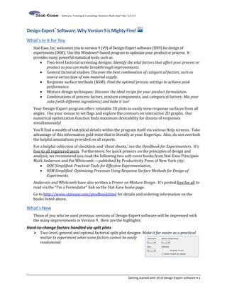
  • 4. Software, Training & Consulting: Statistics Made Easy® Rev. 5/2/14 Getting started with v9 of Design-Expert software  4  Color-coded correlation grid for graph columns: Identify at a glance any factors that are not controlled independently of each other, that is, orthogonally; also useful for seeing how one response correlates to another.* *(Data shown in screen shot comes from historical data detailed in RSM Simplified on NFL sacks versus attributes of defensive linemen.)  Jump to run added to Factors Tool for model graphs: For multidimensional experimental regions, find the slice of interest (containing the point you want to see) at the press of a button.  When jumping to a run, the range expands to include the design point: Use this feature to check how well your model fits—comparing the actual result versus what is predicted via the surface graph (in this case very well—the circled red point is barely beneath the surface!).  Ignored (and missing) runs can be shown on graphs: Good to be reminded that the original design called for this, but for one reason or another, you ignored the outcome (or the response could not be collected, or it was skipped).  Choice to do diagnostic graphs with externally-studentized residuals (now the default): This deletion-diagnostic (vs internally-studentized) provides a more sensitive view of potential abnormalities. B: Trip (mm) D: Fast Shot (mm) 390 395 400 405 Defects(Fraction) 0.00 0.20 0.40 0.60 0.80 1.00 D- D+ Interaction
  • 5. Software, Training & Consulting: Statistics Made Easy® Rev. 5/2/14 Getting started with v9 of Design-Expert software  5 0.00 5.11 10.22 15.33 20.44 0.0 10.0 20.0 30.0 50.0 70.0 80.0 90.0 95.0 Half-Normal Plot |Normal Effect| Half-Normal%Probability A-Homework  Many new icons, such as ones for Clear Points and Pop-Out View on the Diagnostics Tool: Jump to features used frequently more quickly via these handy markers (also they look good!).  Three-component contour graphs in reals: Get a better view of the restrictions placed on your mixture space by the constraints you enter on each component and the total.  Half-normal plot for one-factor categorical experiments with replicates: See at a glance if anything significant emerges. Greater flexibility in data display and export  Descending sort of all individual design layout columns via right-click menu (shown) or double-click on header (toggles with ascending sort—previously the only option): Helpful, for example, when minimum response is desired.  Identify via “Build Type” the predetermined Model, Lack of Fit, Center, and Replicate points in your design layout: Dissect the matrix laid out for optimal (I, D, etc) experiments.  Switch directly between continuous and discrete point type: Sometimes the settings for a factor cannot be easily changed (for example, diameter of molded part)—then it pays to recognize them as discrete, thus enabling the numeric optimizer being set so it will not stray away from specific values.  Ignorable block and/or factor columns: Handy for “what-if” analysis, such as what would have happened if you had not blocked your experiment. A: Water (%) 5.000 B: Alcohol (%) 4.000 C: Urea (%) 4.000 2.000 2.000 3.000 Viscosity (mPa-sec) 40 60 60 80 80 100 120 2 2 2 2
  • 6. Software, Training & Consulting: Statistics Made Easy® Rev. 5/2/14 Getting started with v9 of Design-Expert software  6  Journal feature to export data directly to Microsoft Word or Powerpoint: Fast and formatted for you to quickly generate a presentable report on your experimental results.  Improved copy/paste of Final Equation from the analysis of variance (ANOVA) report to Microsoft Excel: This not only saves tedious transcription of coefficients but it also sets up a calculator for you to ‘plug and chug’, that is, enter into the spreadsheet cells what values for the inputs you’d like to evaluate and see what the model predicts for your response.  From Evaluation and ANOVA screens, the X matrix can be viewed and exported: This is helpful, for example, for copy and paste to R or Matlab where statisticians can do further manipulations for research purposes.  Display full precision of F-test: If just presenting p<0.0001 is not precise enough, show all the decimals.  New XML* script commands for exporting point predictions: Helpful for situations where one wants to automate the transfer of vital outputs from Design-Expert to other programs. *(Extensible Markup Language) More powerful tools for modeling  Design model included in Fit Summary: This can be very helpful for combined designs such as response surface optimizations that include categorical factors (in this case recommending a model that included some cross-product terms of 3rd order, which provided a better fit of the data).
  • 7. Software, Training & Consulting: Statistics Made Easy® Rev. 5/2/14 Getting started with v9 of Design-Expert software  7  All-hierarchical model (AHM) selection: Sort through all possible models up to the one you designed the experiment for, but all the while maintain hierarchy of terms so you do not end up with something ill- formulated. (PS. The alpha out is enforced after AHM is completed by doing a final sweep using backward selection, after which hierarchy is again corrected by the program.)  Non-linear equations involving trigonometric, exponential and other functions allowed for creating deterministic responses (for example—costs) or simulations: This will be especially helpful for setting up more realistic scenarios for students to solve during hands-on workshops for teaching DOE. (PS. Simulator now provides an entry field for ratio of variance between whole and sub plots so trainers can set up split-plot exercises.)  Special quartic Scheffé polynomial included in automatic selection for mixture modeling: Sometimes this added degree (4th!) of non-linear blending helps to better shape the response surface—making it better for predictive purposes. More choices when custom-designing your experiment  Required model points set aside from optional additional ones that may be needed for adequate sizing of the design: Prevents setting up an experiment with too few points to fit the chosen model.  Enter a single factor constraint for response surface designs: Creates a ‘hard’ limit on inputs that cannot go beyond a certain point (such as zero time) physically or operationally.
  • 8. Software, Training & Consulting: Statistics Made Easy® Rev. 5/2/14 Getting started with v9 of Design-Expert software  8  Greater flexibility in setting up models: For example you can now create an optimal model for experiment on mixtures with varying categorical ingredients, some of which can go to zero.* *(See presentation of “Categoric Mixture Components Proportion Going to Zero” by Pat Whitcomb, ENBIS-12, Ljubljana, Slovenia. Slides available on request to stathelp@statease.com.)  Save candidate sets in actuals: More flexibility for customizing your experiment design. More capability for numerical optimization  Include Cpk* as a goal: Meet quality goals explicitly. *(A process capability index widely used for Six Sigma and Design for Six Sigma programs.) Enhanced design evaluation  Random model generator provided to generate a realistic response via a quadratic polynomial with coefficients picked by chance: Use this to play around with how the software presents the analysis—better than just generating random numbers that only fit a mean model.  One-sided option added to FDS* graph: Size your design properly for a verification experiment done to create a QBD** design space. *(Fraction of design space) **(Quality by Design—a protocol promoted by the US Food & Drug Administration (FDA).) Many things made nicer, easier, more configurable and faster  Components that do not vary in a mixture experiment can now be included in the design build—see them highlighted with gray in the layout: Provide a recipe sheet that encompasses the entire formulation, not just what will be manipulated in your study.  Automatically re-sort by run order after re-randomizing: A little feature that saves users a bother.  Diagnostics report now can be sorted by any of the statistics listed: This enables a more informative ordering than by run number (the default).  Faster display of graphs: Great for dazzling your audience with 3D graphs in high resolution.
  • 9. Software, Training & Consulting: Statistics Made Easy® Rev. 5/2/14 Getting started with v9 of Design-Expert software  9  Pop-out views numbered: Makes it easier to distinguish and find the associated view-Tool when re-arranging on your desktop.  Graph state stored with file: Restores setting to the way you liked them.  Improved graphics on Transformation screen: Looks more elegant—better to show off your results via live presentations or webinars.  Fonts on analysis tabs now configurable under Edit Preferences (Dialog Control): Go ahead and make them Comic Sans if you would like to lighten things up. ; ) Safety net expanded—more mistakes caught and ‘heads-ups’ given  Warning when largest effect not selected on half-normal plot: This would not make sense, but it might happen due to, for example, not lassoing points correctly.  Hover Help added to select fields: When your mouse goes over an entry place, the program fills you in with a bit more information on what’s entailed in the feature you are specifying. 0.00 0.10 0.20 0.30 0.40 0.50 0 10 20 30 50 70 80 90 95 99 Half-Normal Plot |Standardized Effect| Half-Normal%Probability B-Flow D-Mud Warning! Largest effect not selected.
  • 10. Software, Training & Consulting: Statistics Made Easy® Rev. 5/2/14 Getting started with v9 of Design-Expert software  10 Niceties that only statisticians might truly appreciate  Mean correction for transformation bias when responses displayed in original scale: All you need to know is that our statisticians figured out how to eliminate a tricky, little-known bias!  Propagation of error (POE) carried out to the second derivative: Makes POE more accurate.  Display confidence bands with or without POE added: Easier to match output with other programs that do not offer POE features like this.  Add unblocked results to evaluation of blocked experiments: Aids in comparing designs on the basis of matrix measures.  Scale to largest estimable effect those normal effects that cannot be otherwise estimated: This can happen when effects become too large compared to the error estimated by chi- square.  Preference now available to display p values to full precision: Previously the program restricted p values to four decimals, which in some cases did not go far enough. Technical stuff only those adept at programming will ‘get’  Automatically generate DTD* files: Now these will always be up to date. *(Document Type Definition)  New command to export runs of a specific type: Particularly useful for verification points. Good news for network administrators  New more flexible and easier-to-use license manager with greater power to serve enterprise users: For example, network ‘seats’ can be checked out to individual laptops and multiple opening of the program on a specific computer will only use one seat.
  • 11. New Designs and Name Changes in V9 of Design-Expert® Software There have been many improvements in Design-Expert (DX9) version 9, notably split-plot designs, which accommodate hard-to-change factors by restricting their randomization into groups. These new designs can be seen at the bottom of the factorial design builder in DX9 (see the box in the screenshot, below right). Randomized designs remain available, but some feature new, more descriptive names, and they have been resorted for easier access. As always in Stat-Ease software, the most commonly used designs get top priority, that is, they are listed in order of usefulness. For a quick overview of the changes, compare the screenshots below. Design-Expert V8 Software – Old Design-Expert V9 Software – New! New Design New Designs
  • 12. Z:ManualDX9DX9-02-1-Simple-Sample-FT.docx5/2/2014 9:18:00 AM Design-Expert® software version 9: Simple Sample Design Version 9 of Design-Expert (DX9) features a “simple sample design” that facilitates a straight-forward analysis of raw data, making it easy to calculate the mean and other statistics that characterize measurements. To illustrate the simple sample tools of DX9, let’s characterize the performance of a motor-shaft supplier. The data, shown below, is a measure of the endplay: 61, 61, 57, 56, 60, 52, 62, 59, 62, 67, 55, 56, 52, 60, 59, 59, 60, 59, 49, 42, 55, 67, 53, 66, 60. The purchaser needs the mean, standard deviation, and 95% confidence interval of this vital attribute. Off the Factorial tab select Simple Sample and, as shown in the screen shot, enter the Response Name “Endplay” and Rows 25 for the number of observations. Then click Continue. The program then presents a blank data entry sheet—a “design layout.” Either type in the data now or open the file “Simple Sample-Motor Shaft.dxpx” that has it pre-entered. Now proceed with the analysis by going to the R1: Endplay node and pressing forward to the ANOVA tab. Design- Expert then presents the needed statistics as seen here. Check out the graphs under Diagnostics (run 20 bears watching as you will see by changing to the Externally Studentized scale for the Resid vs Run chart) as well as the 95%-confidence- banded model graph copied out to the right. Also, take a look at the tool under the Post Analysis node for Point Prediction, in particular the tolerance interval, a very useful statistic for a purchaser who needs to establish incoming specifications. This concludes our feature tour of simple sample tools in DX9. Feel free to explore other tools. If you need more information at any time, press for Tips, Screen Tips off the main menu or push the light bulb icon. Design-Expert® Software Endplay Design Points 95% CI Bands Std # 20 Run # 20 Y = Endplay = 42 CI = (55.6418, 60.2782) Run Number 1 2 3 4 5 6 7 8 9 10 11 12 13 14 15 16 17 18 19 20 21 22 23 24 25 Endplay 40 45 50 55 60 65 70 Simple Sample
  • 13. DX9-02-2-Gen1Factor.docx Rev. 5/2/14 Design-Expert 9 User’s Guide General One-Factor Multilevel-Categoric Tutorial  1 General Multilevel-Categoric One-Factor Tutorial Part 1 – The Basics Introduction In this tutorial you will build a general one-factor multilevel-categoric design using Design-Expert® software. This type of design is very useful for simple comparisons of categorical treatments, such as:  Who will be the best supplier,  Which type of raw material should be selected,  What happens when you change procedures for processing paperwork. If you are in a hurry, skip the boxed bits—these are sidebars for those who want to spend more time and explore things.  Explore response surface methods: If you wish to experiment on a continuous factor, such as time, which can be adjusted to any numerical level, consider using response surface methods (RSM) instead. This is covered in a series of tutorials presented later in the Design-Expert User’s Guide. The data for this example come from the Stat-Ease bowling league. Three bowlers (Pat, Mark, and Shari) are competing for the last team position. They each bowl six games in random order – ideal for proper experimentation protocol. Results are: Game Pat Mark Shari 1 160 165 166 2 150 180 158 3 140 170 145 4 167 185 161 5 157 195 151 6 148 175 156 Mean 153.7 178.3 156.2 Bowling scores Being a good experimenter, the team captain knows better than to simply pick the bowler with the highest mean score. The captain needs to know if the average scores are significantly different, given the variability in individual games. Maybe it’s a fluke that Mark’s score is highest. This one-factor case study provides a good introduction to the power of simple comparative design of experiments (DOE). It exercises many handy features found in Design-Expert software.  Explore other resources: We won’t explain all features displayed in this current exercise because most will be covered in later tutorials. Many other features and outputs are detailed only in the help system, which you can access by clicking Help in the main menu, or in most places via a right click, or by pressing the F1 key (context sensitive).
  • 14. 2  General Multilevel-Categoric One-Factor Tutorial Design-Expert 9 User’s Guide Design the Experiment We will assume that you are familiar with your computer’s graphical user interface and your mouse. Start the program by double clicking the Design-Expert icon. You will then see the main menu and icon bar. Click on File in the main menu. Unavailable items are dimmed. (If you prefer using your keyboard, press the Alt key and underlined letter simultaneously, in this case Alt F.) File menu Select the New Design item with your mouse.  Explore optional ways to select a new design: The blank-sheet icon  on the left of the toolbar is a quicker path to this screen. To try this, press Cancel to re-activate the tool bar. Opening a new design with the blank sheet icon Using either path, you now see four yellow tabs on the left of your screen. The Factorial tab comes up by default. Select Multilevel Categoric for this design. (If your factor is numerical, such as temperature, then you would use the One Factor option under the Response Surface tab.)  Explore what the program tells you in its annotations: Note the helpful description: “Design, also known as “General Factorial”, for 1 to 12 factors where each factor may have a different number of levels.” P.S. If any of your factors are quite hard to control, that is, not easily run at random levels, then consider using the Split- Plot Multilevel Categoric design. However, restricting randomization creates big repercussion on the power of your experiment, so do your best to allow all factors to vary run-by-run as chance dictates. (Design-Expert by default will lay out your design in a randomized run order.)
  • 15. DX9-02-2-Gen1Factor.docx Rev. 5/2/14 Design-Expert 9 User’s Guide General One-Factor Multilevel-Categoric Tutorial  3 Multilevel Categoric design Enter the Design Parameters Leave the number of factors at its default level of 1 but click the entry format Vertical (easier than Horizontal for multiple levels). Enter Bowler as the name of the factor. Tab down to the Units field and enter Person. Next tab to Type. Leaving Type at its default of Nominal, tab down to the Levels field and enter 3. Now tab to L(1) (level one) and enter Pat. Type Mark, and Shari for the other two levels (L2 and L3). Multilevel Categoric design-builder dialog box – completed  Explore screen tips: For details on the options for factor type, click the light bulb icon ( ) in the toolbar to access our context-sensitive screen tips. Screen tips on factor Type Press Continue to specify the remaining design options. In the Replicates field, which becomes active by default, type 6 (each bowler rolls six games). Tab to the “Assign one block per replicate” field but leave it unchecked. Design-Expert now recalculates the number of runs for this experiment: 18.
  • 16. 4  General Multilevel-Categoric One-Factor Tutorial Design-Expert 9 User’s Guide Design options entered Press Continue. Let’s do the easy things first. Leave the number of Responses at the default of 1. Now click on the Name box and enter Score. Tab to the Units field and enter Pins. Response name dialog box – completed At this stage you can skip the remainder of the fields and continue on. However, it is good to gain an assessment of the power of your planned experiment. In this case, as shown in the fields below, enter the value 20 because the bowling captain does not care if averages differ by fewer than 20 pins. Then enter the value 10 for standard deviation (derived from league records as the variability of a typical bowler). Design-Expert then compute a signal- to-noise ratio of 2 (10 divided by 5). Optional power calculator – necessary inputs entered Press Continue to view the happy outcome – power that exceeds 80 percent probability of seeing the desired difference. Results of power calculation Click on Finish for Design-Expert to create the design and take you to the design layout window.
  • 17. DX9-02-2-Gen1Factor.docx Rev. 5/2/14 Design-Expert 9 User’s Guide General One-Factor Multilevel-Categoric Tutorial  5  Explore the program interface: Before moving on, take a look at the unique branching interface provided by Design- Expert for the design and analysis of experiments and resulting optimization. Design-Expert software’s easy-to-use branching interface You will explore some branches in this series of tutorials and others if you progress to more advanced features, such as response surface methods for process optimization. Save the Design When you complete the design setup, save it to a file by selecting File, Save As. Type in the name of your choice (for this tutorial, we suggest Bowling) for your data file, which is saved as a *.dxpx type. Save As dialog box Click on Save. Now you’re protected in case of a system crash. Create a Data Entry Form In the floating Design Tool click Run Sheet (or go to the View menu and select Run Sheet) to produce a recipe sheet for your experiment with your runs in randomized order. A printout provides space to write down the responses. (Note: this view of the data does not
  • 18. 6  General Multilevel-Categoric One-Factor Tutorial Design-Expert 9 User’s Guide allow response entry. To type results into the program you must switch back to the home base – the Design Layout view.) Run Sheet view (your run order may differ)  Explore printing features: It’s not necessary for this tutorial, but if you have a printer connected, you can select File, Print, and OK (or click the printer icon) to make a hard copy. (You can do the same from the basic design layout if you like that format better.) Enter the Response Data When performing your own experiments, you will need to go out and collect the data. Simulate this by clicking File, Exit. Click on Yes if you are prompted to Save. Now re-start Design-Expert and use File, Open Design or click the open file icon on the toolbar)) to open your data file (Bowling.dxpx). You should now see your data tabulated in the randomized layout. For this example, you must enter your data in the proper order to match the correct bowlers. To do this, right-click the Factor 1 (A: Bowler) column header and choose Sort Ascending. Sort runs by standard (std) order Now enter the responses from the table on page one, or use the following screen. Except for run order, your design layout window must look like that shown below.
  • 19. DX9-02-2-Gen1Factor.docx Rev. 5/2/14 Design-Expert 9 User’s Guide General One-Factor Multilevel-Categoric Tutorial  7 Design Layout in standard order with response data entered When you conduct your own experiment, be sure to do the runs and enter the response(s) in randomized order. Standard order should only be used as a convenience for entering pre-existing design data.  Explore advantages of being accurate on the actual run order: If you are a real stickler, replace (type over) your run numbers with the ones shown above, thus preserving the actual bowlers’ game sequence. Bowling six games is taxing but manageable for any serious bowler. However, short and random breaks while bowling six games protects against time-related effects such as learning curve (getting better as you go) and/or fatigue (tiring over time). Save your data by selecting File, Save from the menu (or via the save icon  on the toolbar). Now you’re backed up in case you mess up your data. This backup is good because now we’ll demonstrate many beneficial procedures Design-Expert features in its design layout. For example, right click the Select button. This allows you to control what Design-Expert displays. For this exercise, choose Comments.
  • 20. 8  General Multilevel-Categoric One-Factor Tutorial Design-Expert 9 User’s Guide Select button for choosing what you wish to display in the design layout In the comments column above we added a notation that after run 8, the bowling alley proprietor re-oiled the lane – for what that was worth. Seeing Pat’s scores, the effect evidently was negligible. ; )  Explore entering comments: Try this if you like. If comments exceed allotted space, move the cursor to the right border of the column header until it turns into a double-headed arrow (shown below). Then, just double-click for automatic column re-sizing. Adjusting column size Now, to better grasp the bowling results, order them from low-to-high as shown below by right-clicking the Response column header and selecting Sort Ascending. Sorting a response column (also works in the factor column) You’ll find sorting a very useful feature. It works on factors as well as responses. In this example, you quickly see that Mark bowled almost all the highest games.
  • 21. DX9-02-2-Gen1Factor.docx Rev. 5/2/14 Design-Expert 9 User’s Guide General One-Factor Multilevel-Categoric Tutorial  9 Analyze the Results Now we’ll begin data analysis. Under the Analysis branch of the program (on the left side of your screen), click the Score node. Transform options appear in the main window of Design-Expert on a progressive tool bar. You’ll click these buttons from left to right and perform the complete analysis. It’s a very easy process. The Transform screen gives you the opportunity to select a transformation for the response. This may improve the analysis’ statistical properties. Transformation button – the starting point for the statistical analysis  Explore details on transformations: If you need some background on transformations, first try Tips. For complete details, go to the Help command on the main menu. Click the Search tab and enter “transformations.” As shown at the bottom of the Transform screen above, the program provides data- sensitive advice, so press ahead with the default of None by clicking the Effects tab. Examine the Analysis By necessity, the tutorial now turns a bit statistical. If this becomes intimidating, we recommend you attend a basic class on regression, or better yet, a DOE workshop such as Stat-Ease’s computer-intensive Experiment Design Made Easy. Design-Expert now pops up a very specialized plot that highlights factor A—the bowlers— as an emergent effect relative to the statistical error, that is, normal variation, shown by the line of green triangles.
  • 22. 10  General Multilevel-Categoric One-Factor Tutorial Design-Expert 9 User’s Guide Initial view of the effect of Bowler That is good! It supports what was obvious from the raw results—who bowls does matter.  Explore half-normal plots: If you want to learn more about half-normal plots of effects, work through the Two-Level Factorial Tutorial. To get the statistical details, press the ANOVA (Analysis of Variance) tab. Notice to the far right side of your screen that Design-Expert verifies that the results are significant. ANOVA results (annotated), with context-sensitive Help enabled via right-click menu  Explore the ANOVA report: Now select View, Annotated ANOVA from the menu atop the screen and uncheck () this option. Note that the blue textual hints and explanations disappear so you can make a clean printout for statistically savvy clients. Re-select View, Annotated ANOVA to ‘toggle’ back all the helpful hints. Before moving on, try the first hint shown in blue: “Use your mouse to right click on individual cells for definitions.” For example, perform this tip on the p-value of 0.0006 as shown above (select Help at the bottom of the pop-up menu). There’s a wealth of information to be brought up from within the program with a few simple keystrokes: Take advantage!
  • 23. DX9-02-2-Gen1Factor.docx Rev. 5/2/14 Design-Expert 9 User’s Guide General One-Factor Multilevel-Categoric Tutorial  11 Now click the ‘floating’ (moveable) R-squared Bookmark button (or press the scroll-down arrow at the bottom right screen) to see various summary statistics. Summary statistics  Explore the post-ANOVA statistics: The annotations reveal the gist of what you need to know, but don’t be shy about clicking on a value and getting online Help via a right-click (or try the F1 key). In most cases you will access helpful advice about the particular statistic. Now click the Coefficients Bookmark button to view the output illustrated below. Coefficient estimates Here you see statistical details such as coefficient estimates for each model terms and their confidence intervals (“CI”). The intercept in this simple one-factor comparative experiment is simply the overall mean score of the three bowlers. You may wonder why only two terms, A1 and A2, are provided for a predictive model on three bowlers. It turns out that the last model term, A3, is superfluous because it can be inferred once you know the mean plus the averages of the other two bowlers. Now let’s move on to the next section within this screen: “Treatment Means.” Treatment means Here are the averages for each of the three bowlers. As you can see below, these are compared via pair-wise t-tests in the following part of the ANOVA report.
  • 24. 12  General Multilevel-Categoric One-Factor Tutorial Design-Expert 9 User’s Guide Treatment means You can conclude from the treatment comparisons that:  Pat differs significantly (24.67 pins worse!) when compared with Mark (1 vs 2)  The 2.5 pins mean difference between Pat and Shari (1 vs 3) is not significant (nor is it considered important by the bowling team’s captain – recall in the design specification for power that a 10-pin difference was the minimum of interest)  Mark differs significantly (22.17 pins better!) when compared with Shari (2 vs 3).  Explore the Top feature: Before moving ahead, press Top on the floating Bookmark. This is a very handy way of moving through long reports, so it’s worth getting in the habit of using it. Back to the top Analyze Residuals Click the Diagnostics tab to bring up the normal plot of residuals. Ideally this will be a straight line, indicating no outlying abnormalities.  Explore the ‘pencil test’: If you have a pencil handy (or anything straight), hold it up to the graph. Does it loosely cover up all the points? The answer is “Yes” in this example – it passes the “pencil test” for normality. You can reposition the thin red line by dragging it (place the mouse pointer on the line, hold down the left button, and move the mouse) or its “pivot point” (the round circle in the middle). However, we don’t recommend you bother doing this – the program generally places the line in the ideal location automatically. If you need to re-set the line, simply double-click your left mouse button over the graph. Notice that the points are coded by color to the level of response they represent – going from cool blue for lowest values to hot red for the highest. In this example, the red point is Mark’s outstanding 195 game. Pat and Shari think Mark’s 195 game should be thrown out because it’s too high. Is this fair? Click this point so it will be highlighted on this and all the other residual graphs available via the Diagnostics Tool (the ‘floating’ palette on your screen).
  • 25. DX9-02-2-Gen1Factor.docx Rev. 5/2/14 Design-Expert 9 User’s Guide General One-Factor Multilevel-Categoric Tutorial  13 Normal probability plot of residuals (195 game highlighted)  Explore the Top feature: Notice on the Diagnostics Tool that they are “studentized” by default. This converts raw residuals, reported in original units (‘pins’ of bowling in this example), to dimensionless numbers based on standard deviations, which come out in plus or minus scale. More details on studentization reside in Help. Raw residuals can be displayed by choosing it off the down-list on the Diagnostics Tool shown below. Check it out! Other ways to display residuals In any case, when runs have greater leverage (another statistical term to look up in Help), only the Studentized form of residuals produces valid diagnostic graphs. For example, if Pat and Shari succeed in getting Mark’s high game thrown out (don’t worry – they won’t!), then each of Mark’s remaining five games will exhibit a leverage of 0.2 (1/5) versus 0.167 (1/6) for each of the others’ six games. Due to potential imbalances of this sort, we advise that you always leave the Studentized feature checked (as done by default). So if you are on Residuals now, go back to the original choice that came up by default (externally* studentized). *P.S. Another aspect of how Design-Expert displays residuals by default is them being done “externally”. This is explored in the Two-Level Factorial Tutorial. For now, suffice it to say that the program chooses this form of residual to provide greater sensitivity to statistical outliers. This makes it even more compelling not to throw out Mark’s high game. On the Diagnostics Tool, select Resid. vs. Pred. to generate a plot of residuals for each individual game versus what is predicted by the response model.  Explore an apocryphal story: Supposedly, “residuals” were originally termed “error” by statisticians, but the management people got upset at so many mistakes being made! Let’s make it easier to see which residual goes with which bowler by pressing the down-list arrow for the Color by option in the Diagnostics Tool and selecting A:Bowler.
  • 26. 14  General Multilevel-Categoric One-Factor Tutorial Design-Expert 9 User’s Guide Residuals versus predicted values, colored by bowler The size of the studentized residual should be independent of its predicted value. In other words, the vertical spread of the studentized residuals should be approximately the same for each bowler. In this case the plot looks OK. Don’t be alarmed that Mark’s games stand out as a whole. The spread from bottom-to-top is not out of line with his competitors, despite their protestations about the highest score (still highlighted). Bring up the next graph on the Diagnostics Tool list – Resid. vs Run (residuals versus run number). (Note: your graph may differ due to randomization.) Residuals versus run chart (Note: your graph may differ due to randomization) Here you might see trends due to changing alley conditions (the lane re-oiling, for example), bowler fatigue, or other time-related lurking variables.  Explore repercussion of possible trends: In this example things look relatively normal. However, even if you see a pronounced upward, downward, or shift change, it will probably not bias the outcome because the runs are completely randomized. To ensure against your experiment being sabotaged by uncontrolled variables, always randomize! More importantly in this case, all points fall within the limits (calculated at the 95 percent confidence level). In other words, Mark’s high game does not exhibit anything more than common-cause variability, so it should not be disqualified. Design-Expert® Software Score Color points by level of Bowler: Pat Mark Shari Std # 11 Run # 14 X: 14 Y: 2.175 Run Number ExternallyStudentizedResiduals Residuals vs. Run -4.00 -2.00 0.00 2.00 4.00 1 3 5 7 9 11 13 15 17
  • 27. DX9-02-2-Gen1Factor.docx Rev. 5/2/14 Design-Expert 9 User’s Guide General One-Factor Multilevel-Categoric Tutorial  15 View the Means and Data Plot Select the Model Graphs tab from the progressive tool bar to display a plot containing all the response data and the average value at each level of the treatment (factor). This plot gives an excellent overview of the data and the effect of the factor levels on the mean and spread of the response. Note how conveniently Design-Expert scaled the Y axis from 140 to 200 pins in increments of 10. One-factor effects graph with Mark’s predicted score (mean) highlighted The squares in this effects plot represent predicted responses for each factor level (bowler). Click the square representing Mark’s mean score as shown above. Notice that Design- Expert displays the prediction for this treatment level (reverting to DOE jargon) on the legend at the left of the graph. Vertical ‘I-beam-shaped’ bars represent the 95% least significant difference (LSD) intervals for each treatment. Mark’s LSD bars don’t overlap horizontally with Pat’s or Shari’s, so with at least 95% confidence, Mark’s mean is significantly higher than the means of the other two bowlers.  Explore other points on the model graph: Oh, by the way, maybe you noticed that the numerical value for the height of the LSD bar appeared when you clicked Mark’s square. You can also click on any round point to see the actual scores. Check it out! Pat and Shari’s LSD bars overlap horizontally, so we can’t say which of them bowls better. It seems they must spend a year in a minor bowling league and see if a year’s worth of games reveals a significant difference in ability. Meanwhile, Mark will be trying to live up to the high average he exhibited in the tryouts and thus justify being chosen for the Stat-Ease bowling team. That’s it for now. Save your results by going to File, Save. You can now Exit Design-Expert if you like, or keep it open and go on to the next tutorial – part two for general one-factor design and analysis. It delves into advanced features via further adventures in bowling.
  • 28. 16  General Multilevel-Categoric One-Factor Tutorial Design-Expert 9 User’s Guide General One-Factor Tutorial (Part 2 – Advanced Features) Digging Deeper Into Diagnostics (Caution: Only the more daring new users should press ahead from here—those who like to turn over every rock to see what’s underneath, that is—the types who are curious to know everything there is to know. If that’s not you, skip the rest and go on to another tutorial if it offers feature you need for your particular experiment.) If your bowling data is active in Design-Expert® software from Part 1 of this tutorial, continue on. If you exited the program, re-start it and use File, Open Design to open data file (Bowling.dxpx). Otherwise, set up this data file as instructed above in our General One-Factor Tutorial (Part 1 – The Basics). Then, under the Analysis branch (you may already be here) click the Score node and press the Diagnostics tab. We’re now going to look at a new graph in the Diagnostics Tool. Click the Influence option on the Diagnostics Tool palette. Then click on DFFITS. This statistic, which stands for difference in fits, measures the change in each predicted value that occurs when that response is deleted. The larger the absolute value of DFFITS, the more it influences the fitted model. (For more details on this statistic and the related deletion diagnostic, DFBETAS, see our program Help or refer to Raymond Myers’ Classical and Modern Regression with Applications, 2nd Edition (PWS Pub. Co., 1990).) DFFITS graph (your graph may differ due to random runs) Notice that one point lies above the rest. (The pattern on your graph may differ from what we show here due to randomized run order, but this isn’t a concern in this discussion.) The top-most point is Mark’s high game, which earlier created controversy, particularly among competitors Pat and Shari. Mark’s point falls far below a relatively conservative high benchmark of plus-or-minus two for the DFFITS. So, taking all other diagnostics into consideration, we don’t advise that this particular run be investigated further.
  • 29. DX9-02-2-Gen1Factor.docx Rev. 5/2/14 Design-Expert 9 User’s Guide General One-Factor Multilevel-Categoric Tutorial  17 Nevertheless, for purposes of learning how to use new Design-Expert software features, right-click Mark’s top point with your mouse and select Highlight Point as shown below. Highlighting a point Myers demonstrates mathematically that the DFFITS statistic is really the externally studentized residual multiplied by high leverage points. Click the Leverage button and you’ll see that all runs exhibit equal leverage here because an equal number of runs were made at each treatment level (all three bowlers rolled six games each). Leverages Therefore, this DFFITS exhibits a pattern identical to that shown on the externally studentized residual graph, which you studied in the preceding tutorial. The reason we’re reviewing this is to set the stage for what you’ll do later in this tutorial – unbalance the leverages to make this session more significant for diagnostic purposes.  Explore the Pop-Out View feature: Now is a good time to go back to the DFFITS plot and press the Pop-Out View button the very bottom of the Diagnostics Tool. Pop-Out View button Next go back via the Diagnostics button to the Resid. vs Run plot and verify the statement above that in this case these two plots (DFFITs and residuals versus run) exhibit the same pattern. (You may need to press Alt-Tab to get the windows you want on the same screen.)
  • 30. 18  General Multilevel-Categoric One-Factor Tutorial Design-Expert 9 User’s Guide Demonstration of pop-out view to see two plots side by side You’d best now close out the pop-out view by pressing the X at the upper right corner. Otherwise your screen will get too messy. Here’s one final Design-Expert software feature for you before we leave the Diagnostics Tool: Click the Report button to get a table of statistics case-by-case in standard order for the entire experiment. For those of you who prefer numbers over pictures (statisticians for sure!), this should satisfy your appetite. Notice that Mark’s high 195 game is highlighted in blue text as shown below. Report with case statistics used for preceding diagnostics graphs Remember, you can right-click any value in reports of this nature within Design-Expert software to view context-sensitive Help with statistical details. Modifying the Design Layout Design-Expert offers great flexibility when modifying data in its design layout. We’ll see in this bowling scenario how our software allows you to modify an existing design with added blocks and factor levels. The outcome of the bowling match appears to be definitive, especially from Mark’s perspective. But Pat and Shari demand one more chance to prove themselves worthy of the
  • 31. DX9-02-2-Gen1Factor.docx Rev. 5/2/14 Design-Expert 9 User’s Guide General One-Factor Multilevel-Categoric Tutorial  19 team. They still think Mark’s high 195 game was a fluke, even though this isn’t supported by the diagnostic analysis. Mark objects and a dispute ensues. Attempting compromise, the team captain decides to toss out the highest and lowest games for each of the three bowlers and replace them with two new scores each. But Ben, a newly hired programmer and avid bowler, arrives at the alley and is allowed to participate in this second block of runs. (Yes, this makes little sense, but it will add some interest to this tour of Design-Expert’s flexibility for design and analysis of experiments – no matter how convoluted they become in actuality.) It quickly becomes apparent that this new kid does things differently. He’s a lefty with a huge hook that’s hard to control. To aggravate this variability, Ben does something very different from other bowlers – he does not put his thumb in the ball’s hole made for that purpose. When Ben’s odd approach works, the pins go flying. But as likely as not, that ball slides off into the left gutter or careens over the edge on the right. The results for Ben and the three original bowling team candidates are below. Block Game Pat Mark Shari Ben 1 1 160 165 166 NA 1 2 150 180 158 NA 1 3 140 170 145 NA 1 4 167 185 161 NA 1 5 157 195 151 NA 1 6 148 175 156 NA 2 1 162 175 163 200 2 2 153 180 166 130 Bowling scores with high and low games replaced by two new games (plus a new guy) To enter this new data (and ignore some of the old), click the Design node near the upper left of your screen. You should now see the bowling data from the first tutorial. Mark’s high 195 game remains highlighted in blue text (assuming you clicked on it as instructed on page 2 of this tutorial while performing the diagnostics). Right click the Select column header and click Block. This design attribute is now needed to accommodate the new bowler’s (Ben’s) incoming score data.
  • 32. 20  General Multilevel-Categoric One-Factor Tutorial Design-Expert 9 User’s Guide Selecting block to display it as a column in the design layout Right click the Response column header and choose Sort Ascending. You did this before in Part 1 so you now have this feature mastered…we hope. ; ) Mark’s best game now drops to the very bottom. Let’s single him out first to placate Pat and Shari. Right-click the square button at the left of the last row (Mark’s 195 score). Click Set Row Status, then Ignore as shown below. Ignoring Mark’s high game By the way, it’s OK to change your mind when modifying your design layout: You can ‘un- ignore’ a row by clicking Set Row Status, Normal. Now let’s really get Pat’s and Shari’s hopes high by excluding their low games from consideration. Click the square button (in the Select column) to the left of the top row (Pat’s low 140 game) and, while pressing down the Shift key, also click the button in the Select column’s second row (Shari’s low 145 game). Release the Shift key. Keep your mouse within the Select column’s first or second row, right-click and choose Set Row Status, Ignore for these two low games, as shown below.
  • 33. DX9-02-2-Gen1Factor.docx Rev. 5/2/14 Design-Expert 9 User’s Guide General One-Factor Multilevel-Categoric Tutorial  21 Ignoring the low games for Pat and Shari Now move down a few rows and click the square button in the Select column’s row showing Mark’s low 165 game. Notice the two rows below Mark’s low 165 game – the high games for Shari (166) and Pat (167). It’s now time for Shari and Pat to pay the price for complaining. While first pressing and holding down the Shift key, click the following two square buttons in the Select column’s row: Shari’s high 166 game and Pat’s high 167 game. Release the Shift key. Three rows should now be highlighted in light blue as shown below. Keep your mouse within the Select column’s highlighted three rows, right-click and choose Set Row Status, Ignore. Ignoring Mark’s low game and the high games for Shari and Pat Now let’s restore the original layout order. Right-click the Factor 1 (A: Bowler) column header, then choose Sort Ascending. Compare your screen with what we show below. If there are differences, fix them now to match this screenshot. However, remember that the run number is random, so you don’t need to fix that.
  • 34. 22  General Multilevel-Categoric One-Factor Tutorial Design-Expert 9 User’s Guide Back to standard order after low and high games ignored for each bowler Now create a new block (needed for the second round of bowling) by right-clicking the Block column header and choosing Edit Info as shown below. Creating a new block You’ll see a form allowing you to assign names to the block(s). Don’t bother doing this now. As shown below, change Number of Blocks at the top to 2. Press the Tab key to see the change take effect. (If the name field truncates, click and move the right border of the column header to re-size it.)
  • 35. DX9-02-2-Gen1Factor.docx Rev. 5/2/14 Design-Expert 9 User’s Guide General One-Factor Multilevel-Categoric Tutorial  23 Adding a second block of runs Click OK. It seems that nothing changed, but actually the program now knows that you will be conducting another block of runs. Now you are ready to begin adding and/or duplicating rows. This can be accomplished in different ways, depending on your ingenuity. We’ll follow routes revealing as many of the editing features as possible, although they may not demonstrate the most elegant approaches. As shown below, right click the Select column’s square button at the left of the first row (Pat’s 160 game) to bring up the editing menu. Click the first selection, Insert Row. Inserting a new row You now see a new row containing blanks for the bowler and the score. (Don’t worry if it’s being ignored – crossed out, that is – for the moment.) Click the first row’s block cell directly below the block field header, then click the list arrow. Select Block 2 as shown below. Changing the block number Click the blank field for bowler and press the list arrow (). Select Pat. (We’re using categorical factors here, but if this were a numerical field, you’d enter a value.)
  • 36. 24  General Multilevel-Categoric One-Factor Tutorial Design-Expert 9 User’s Guide Entering a categorical value for factor Again, right-click the Select column’s square button at the left of the first row to bring up the editing menu as shown below. Click Duplicate. Duplicating a row Design-Expert may pop up a warning like the one shown below. Warning about categoric contrasts The program is recognizing a potential problem here and is alerting you that only one bowler is in the second block. You need not worry at this stage because you will be adding others. Click the check option Do not show this warning again. This will save you aggravation later. Don’t worry – you will not be unprotected indefinitely. This warning will be re-enabled the next time you start the program. Turning off a warning (it will come back the next time you run the program) Press OK to proceed. Right-click the Block column header and choose Sort Ascending. Two new rows are now seen at the bottom of your design layout. We need two new rows apiece for Shari and Mark. Let’s simply duplicate Pat’s two new rows and update the names. Do this by first clicking the Select column’s square button at the left of Pat’s first new row, so it is highlighted. Then while holding down the Shift key, click the Select column’s square button at the left of Pat’s second new row. Both rows should now be highlighted. (This is a bit tricky, but it saves time.)
  • 37. DX9-02-2-Gen1Factor.docx Rev. 5/2/14 Design-Expert 9 User’s Guide General One-Factor Multilevel-Categoric Tutorial  25 Now right-click any Select column’s square button at the left of the highlighted block and select Duplicate. (If the warning screen pops up again, click OK.) Duplicating a block of rows In the first duplicated row, click the field for Bowler and select Mark. Changing name of bowler Do the same for the last row. You now should have two new rows for both Pat and Mark. Click the Select column’s square button at the left of Mark’s first new row, so it is highlighted. Then while holding down the Shift key, click the Select column’s square button at the left of Mark’s second new row. Both rows should now be highlighted. As before, right-click any Select column’s square button at the left of the highlighted block and select Duplicate. Duplicating two more rows In the first duplicated row, click the field for Bowler and select Shari. Do the same for the last row.
  • 38. 26  General Multilevel-Categoric One-Factor Tutorial Design-Expert 9 User’s Guide Completing lineup for block 2 – the second round of bowling But what about the new kid – Ben? We need to identify him as a new competitor in this bowling contest. Do this by right-clicking the header for Bowler and selecting Edit Info. Getting ready to add a new level for the factor Change Number of Levels to 4 (see below left). Adding another bowler Press Tab once. Click the field intersecting at Name column and row 4 (below right). Type the name Ben. Entering the new bowler Press OK. Now duplicate two more rows by clicking the Select column’s square button at the left of the first of Shari’s two new games at the bottom of the list. While holding down the Shift key, click the Select column’s square button at the left of the last run. Finally, right-click any Select column’s square button at the left of the highlighted block and select Duplicate. In both of these new duplicated rows, click the fields for Bowler and select Ben.
  • 39. DX9-02-2-Gen1Factor.docx Rev. 5/2/14 Design-Expert 9 User’s Guide General One-Factor Multilevel-Categoric Tutorial  27 Ben now on the list as a bowler An important aside: Always randomize your run orders for actual experiments. For purposes of this tutorial, this will just be a bother, so do this only if you wish to try it out, but it’s very easy to do – simply right-click the Run column-header and do this for Block 2 as shown. How to randomize the run order in the second block To make it easier to enter the results, right-click the Factor 1 (A: Bowler) column header and Sort Ascending. Then right-click the Block column header and Sort Ascending. Now enter the eight new scores as shown below. Data entered for second block of games Go ahead now and re-analyze your data by clicking the Score node under Analysis. Move through Transform and click on the Effects tab. A warning pops up that the design is not “orthogonal.”
  • 40. 28  General Multilevel-Categoric One-Factor Tutorial Design-Expert 9 User’s Guide Warning about design now being non-orthogonal This is a mathematical artifact of our ad hoc addition of runs in a second block. It will not create any material impact on the outcome so just press on via OK and click the square appearing at the end of the green triangles (error estimates) on the half-normal plot of effects. This puts A-Bowler in your model. Bowler picked on half-normal plot of effects Proceed to ANOVA (overlooking this model being not significant) and then to Diagnostics. As you will see, something is abnormal about this data. Do you notice that the residuals now line up very poorly, especially at the extreme points as shown below? On the floating Diagnostics Tool change Color by to A: Bowler.
  • 41. DX9-02-2-Gen1Factor.docx Rev. 5/2/14 Design-Expert 9 User’s Guide General One-Factor Multilevel-Categoric Tutorial  29 Diagnostics for bowling results – part two: Normal plot with poorly aligned residuals Now (referring to the color key at the left of the plot) you see that the results from Ben do not fit with the others (his games are the two outliers – low and high). Considering his odd, unstable style of bowling, this should be no surprise. Click the Resid. vs Run button to bring up the externally studentized residuals – a good tool for detecting outliers. Drag your mouse over Ben’s residuals at the far right. Ben’s games highlighted for being outliers Both points should now be highlighted. We must ignore or delete them. (Sorry Ben, odd behavior by programmers is considered normal at Stat-Ease, but not when it comes to bowling!) Click the Design node (upper left) to get back to the home base of the design layout. Notice that Ben’s games are conveniently highlighted in blue text so they can easily be deleted.  Explore an option for ignoring data: It provides no advantage in this case, which features only one response measure, but you can ignore a specific result by right-clicking that cell and setting Set Cell Status to Ignore as shown below.
  • 42. 30  General Multilevel-Categoric One-Factor Tutorial Design-Expert 9 User’s Guide Ignoring a single cell – an option that’s not recommended for this case In this case you could ignore his entire runs (we explained how to do this earlier). Better yet, simply delete them altogether. No offense to Ben, but given that he only bowled two games and his unorthodox style creates such abnormal variability, it is best now to click the Select column’s square button at the left of his first score of 200 (making him feel really bad ), shift-click the button below it for the second game of 130 (not so sorry to see this gone!), then without moving your mouse, right-click and select Delete Row(s). Deleting Ben’s games Click Yes on the warning that pops up about deleting rows (a safety precaution) and OK when asked to re-sequence the runs to fill the gap. Then go ahead and re-analyze the results. It turns out that the added games cause no change in the overall conclusions as to who’s the better bowler. Mark remains on top. It would now be appropriate to recover the low and high games for each bowler from block 1. Because this data was not deleted, only ignored, getting it back is simply a matter of right-clicking to the left of each of the six suspect rows and changing Set Row Status to Normal. (Or, if you’re adept at manipulating lines of text or data with your mouse, do all rows at once using a click and shift-click.) Give this a try! Then re-analyze one last time. By working through this exercise, you now see how easy it is to manipulate Design-Expert’s design layout. P.S. Still feeling bad about deleting Ben’s scores? Don’t worry – he gets to bowl with Pat and Shari in a lesser league. After bowling for an entire year (roughly 100 games), it will become clear whether Ben’s crazy way of bowling will pay off by achieving a good average overall. After all, his 2 game average of 165 wasn’t so bad, just inconsistent (high variability). With more data, his true ability will become more apparent.
  • 43. DX9-02-3-Gen2Factor.docx Rev. 5/2/14 Design-Expert 9 User’s Guide General Multilevel-Categoric Factorial Tutorial  1 General Multilevel-Categoric Factorial Tutorial Part 1 – Categoric Treatment Introduction – A Case Study on Battery Life Design-Expert® software version 9 offers a “Multilevel Categoric” option, also known as a “general factorial” on the “Factorial” design tab. If you have completed the General One- Factor Multilevel-Categoric Tutorial (recommended), you’ve seen how this option handles one multilevel, categorical factor. In this two-part tutorial you will learn how to set up a design for multiple categorical factors. Part 2 shows you how to convert truly continuous factors, such as temperature, from categorical to numerical. With this you can generate response surface graphs that provide a better perspective of your system. If you are in a hurry, skip the boxed bits—these are sidebars for those who want to spend more time and explore things. The experiment in this case, which comes from Montgomery’s Design and Analysis of Experiments, seeks consistently long life in a battery that will be subjected to extremes in ambient conditions. It evaluates three materials (factor A) at three levels of temperature (factor B). Four batteries are tested at each of the nine two-factor combinations in a completely randomized design. The responses from the resulting 36 runs are shown below. Material Type Temperature (deg F) 15 70 125 A1 130 155 34 40 20 70 74 180 80 75 82 58 A2 150 188 136 122 25 70 159 126 106 115 58 45 A3 138 110 174 120 96 104 168 160 150 139 82 60 General factorial design on battery life (data in units of hours) The following questions must be answered: • How does material type and temperature affect battery life? • Do any materials provide uniformly long life regardless of temperature? The big payoff comes if the battery can be made more tolerant to temperature variations in the field. This case study provides a good example of applying statistical DOE for robust product design. Let’s get started on it! Design the Experiment To build the design, choose File, New Design as shown below (or to save strokes, simply click the blank-sheet icon () on the toolbar).
  • 44. 2  General Multilevel-Categoric Factorial Tutorial Design-Expert 9 User’s Guide Starting a new design via menu (option: click blank-sheet icon () on the toolbar) Then from the default Factorial tab, click Multilevel Categoric. Choose 2 as the number of factors. If you are in Horizontal entry mode, change it to Vertical. (Design-Expert will remember this the next time you set up a design.) Selecting number of factors for multilevel-categoric general-factorial design Enter Material for factor name A (Categoric). Key in the word Type as your Units. Enter the value 3 for the number of levels. Change the treatment names to A1, A2 and A3. Notice that Type in the far left column defaults to Nominal (named) as opposed to ordinal (ordered). This difference in the nature of factors affects how Design-Expert codes the categorical levels, which changes the model coefficients reported under ANOVA in the subsequent response analysis. Your design should now appear as that shown below. Entering material as a nominal factor  Explore details in Help on general factorial designs: Tutorials such as this one on general factorials will quickly get you up to speed on how to use Design-Expert software, but it does not serve as a statistical primer for design and analysis of experiments. If you crave such details, Help is at your fingertips! For example, go to Help, Contents and work your way down the tree structure through the factorial branches to General (Multi-Level) Factorial Design. Note the details on the distinction in categoric contrasts (Nominal vs Ordinal).
  • 45. DX9-02-3-Gen2Factor.docx Rev. 5/2/14 Design-Expert 9 User’s Guide General Multilevel-Categoric Factorial Tutorial  3 Help on general factorial design Close Help by pressing X on its window. Now enter factor B data by keying in Temperature for factor name B (Categoric), deg F for units, 3 for the number of levels, and 15, 70 and 125 for the levels. Press Nominal, click the arrow on the drop list, then choose Ordinal as shown below. This change from Nominal to Ordinal indicates that although this factor is being treated categorically (for example, due to controls offering only the three levels), temperature is really a continuous factor. Click Continue at the screen’s far lower right. Entering information on factor B Enter 4 for replicates. The number of runs (36) won’t be updated until you press the Tab key or move from the cell. Leave the blocks option alone because these experiments are completely randomized.
  • 46. 4  General Multilevel-Categoric Factorial Tutorial Design-Expert 9 User’s Guide Entering the number of replicates Click Continue to move on to the entry screen for responses. Leave the default responses at 1. Enter name as Life and units as hours. Now we will walk you through a calculation of power – the ability of your experiment to detect meaningful differences in treatments. If you do too few runs and under-power your experiment, an important change in response (the “signal”) will become obscured by normal system/test variation (the “noise”). That would be a waste of time and materials. Design-Expert makes the calculation of power easy and puts it in upfront in the design- building process so you have a chance to bolster your experiment, if necessary. Let’s assume that battery life must improve by at least 50 hours to be of any interest and that quality control records produce a standard deviation of 30. Enter these values as shown below, Tab (or click) out of 30, and Design-Expert then calculates the signal to noise ratio. Response entry screen Press Continue to see the power of this design for the difference that the engineers hope to detect, at a minimum. It is calculated to be 94.5 % probability of seeing a difference (delta) as small as 50 hours. This exceeds the rule-of-thumb for power of 80 % at a minimum, thus it can be concluded that the planned design will suffice. Power calculation Click Continue to complete the design specification process. Design-Expert now displays the 36 runs (in random order) from the replicated 3x3 factorial design. Analyze the Results To save time, simulate the experimental results by right-clicking the response header and selecting Simulate.  Explore simulation tools: A heads-up for statistics educators: You can build your own simulations via the Design Tools. Feel free to bring up the controls for this and press Help for details on using it.
  • 47. DX9-02-3-Gen2Factor.docx Rev. 5/2/14 Design-Expert 9 User’s Guide General Multilevel-Categoric Factorial Tutorial  5 Choosing a simulation Then choose Load an existing simulation. Finally, click the file named Battery.simx and Open it. If this file does not appear, e-mail support@statease.com for help. You should now see data from the experiment . This is a good time to preserve your work: Select File and Save As. Change the file name to Battery.dxpx and Save. Now go to the Analysis branch of the program and click the node labeled R1:Life. This brings up options for applying response transformations. First step in the analysis – transformation options Leave the transformation at the default of “None” and go ahead and click the Effects button displayed next in the toolbar for response analysis. Design-Expert now provides an initial effect selection and displays it graphically on a specialized statistical plot called a “half- normal.”
  • 48. 6  General Multilevel-Categoric Factorial Tutorial Design-Expert 9 User’s Guide Initial effect selection  Explore details on how the half-normal plot is constructed for general factorial designs: The program displays the absolute value of all effects (plotted as squares) on the bottom axis. The procedure is detailed in a presentation by Patrick Whitcomb on “Graphical Selection of Effects in General Factorials” (2007 Fall Technical Conference co- sponsored by the American Society for Quality and the American Statistical Association) – contact Stat-Ease for a copy. Design-Expert pre-selected two outstanding effects – the main effects of factors A and B. You can, and in this case should, modify the default effect selection. Move your mouse cursor over the unlabeled square and click it. (Note that this goes both ways, that is, you can deselect chosen effects with a simple mouse click.) Another effect chosen Interaction AB is now identified. Notice that Design-Expert adjusts the line to exclude the chosen effects. You will gain more practice on the use of half-normal plots for picking effects in the Two-Level Factorial Tutorial. It’s best to now press ahead in this case.  Explore the Effects List: For statistical details, press the Effects List bar on the floating Effects Tool. Effects list
  • 49. DX9-02-3-Gen2Factor.docx Rev. 5/2/14 Design-Expert 9 User’s Guide General Multilevel-Categoric Factorial Tutorial  7 Notice the designation “M” for the selected model terms A, B and AB and the “e” next to the pure error line in this statistical spreadsheet. You may be wondering why there are so many estimates of pure error. (If not, skip ahead!) Each subgroup of 4 replications provides 3 degrees of freedom (“df”) of pure error. This was done for all 9 factor combinations (3x3) which yields 27 df (= 3*9) in total for estimating pure error. This screen provides many features for model selection, which will be covered in tutorials on response surface methods (RSM). Click the ANOVA tab to see the analysis of variance for this chosen model. If you do not see annotations in blue text as shown below, select View, Annotated ANOVA. Annotated ANOVA Report  Explore the other details provided under the ANOVA tab: Scroll down or press bookmarks on the floating tool to see post-ANOVA statistics such as R-Squared. As you can conclude for yourself by reading the annotations, the results look good. Further down the report are details of the model based on nominal contrasts. We provide a breakdown on this in the Experiment Design Made Easy workshop. To keep this tutorial moving, it’s best not to get bogged down in the mathematics of modeling categorical factors, so press ahead Open the Diagnostics tab and examine the residual graphs. By default you see the normal plot of residuals, which ideally fall more-or-less in line. The pattern here is a bit askew but not badly abnormal, so do not worry.
  • 50. 8  General Multilevel-Categoric Factorial Tutorial Design-Expert 9 User’s Guide Normal plot of residuals – looks OK  Explore all the other diagnostic plots: Take some time now to click your way down the floating tool and then over to the Influence side for viewing every one of the diagnostics plots and the final report. The tedious, but necessary, model-fitting and statistical validation is now completed, so you are free and clear to finally assess the outcome of the experiment and decide whether any materials provide uniformly long battery-life regardless of temperature. Present the Experimental Findings Click the Model Graphs to view the long-awaited results. Design-Expert automatically presents the AB interaction plot – identified by the Term window on the floating Factors Tool. Default model graph – interaction plot with A on bottom (X1) axis
  • 51. DX9-02-3-Gen2Factor.docx Rev. 5/2/14 Design-Expert 9 User’s Guide General Multilevel-Categoric Factorial Tutorial  9  Explore an over-simplified factor plot: Choose the One Factor plot view via the View menu, or by simply pressing the appropriate button on the floating Graphs Tool. Another way to bring up a one-factor plot (the main effect of A or B, in this case) is by clicking the down-list arrow () for the Term selection on the Factors Tool. Try all these approaches if you like, but expect to be warned about presenting main effects of factors that interact. This can be very misleading. In this case it will be a mistake to look at either material or temperature effects alone, because one factor depends on the other. However, while you are at this, explore options on the Factors Tool for B: Temperature. Press the three buttons from left to right and notice how much the effects change due to the interaction. The press avg. Viewing each Temperature and then its average for the effect plot of Material Notice how the least significant difference (LSD) bars contract after the averaging. But nevertheless, this is not helpful because it obscures the interaction. On the Graphs Tool press the Interaction plot to bring back the true picture. Graphs tool – interaction plot selected Right click the Temperature factor on the floating Factors Tool and change it to the X1 Axis, thus producing an interaction graph with the ordinal factor displayed in a continuous manner and the nominal factor (material) laid out discretely as separate lines. This makes it easier to interpret your results. Effect graph with temperature on bottom axis
  • 52. 10  General Multilevel-Categoric Factorial Tutorial Design-Expert 9 User’s Guide  Explore how the software identifies points: Click the highest point (green) at the upper left of the graph. Point highlighted for identification Note how to the left of the plot the software identifies the point by:  Standard order number (2) and run number (randomized)  Actual response “Y” (188)  Factor levels “X” (temperature of 15 with material A2). The actual results are represented by various-colored circles. If there are multiples, the program displays a number; in this case quite a few labeled “2”. Click these points multiple times to see details on each and every one of them. You can also click on the non-circular symbols (square, triangle or diamond) to display the predicted outcome and least significant difference (LSD). Try this! To produce a cleaner looking plot, go to View and deselect Show Legend. Now let’s do some more clean-up for report purposes: Right-click over the graph and select Graph Preferences. Right-click menu selection for graph preferences Now click the All Graphs tab and turn off (uncheck) the Show design points on graph option, as shown below. Turning off design points Press OK.  Explore copy/past to Microsoft Word (or the like): This is an optional sidetrack on this tutorial: To have your graph look like that shown below for reporting purposes, do the following: Edit, Copy from Design-Expert, then Paste into Microsoft Word.
  • 53. DX9-02-3-Gen2Factor.docx Rev. 5/2/14 Design-Expert 9 User’s Guide General Multilevel-Categoric Factorial Tutorial  11 Clean-looking interaction graph From this graph you can see that all three materials work very well at the low temperature (15 degrees). Based on the overlapping LSD bars, it would be fair to say that no material stands out at this low temperature end of the scale. However, the A1 material clearly falls off at the 70 degree temperature, which would be encountered most often, so it must be rejected. None of the materials perform very well at the highest temperature (125 degrees), but the upper end of the LSD bar for A2 barely overlaps the bottom end of the LSD bar for A3. Therefore, with respect to temperature sensitivity, material A3 may be the most robust material for making batteries. Finally, if you do have an opportunity to present graphics in color, here’s a dazzling new and easy way to display general factorial effects with Design-Expert: Click 3D Surface on the floating Graphs Tool. Now place your mouse cursor on the graph – notice that it changes to a hand (). While pressing the left mouse button, spin the graph so the temperature axis is at the bottom. (Alternatively, to match our graph most precisely, select View, Show Rotation and enter coordinates of h (horizontal) 20 and v (vertical) 80.) B: Temperature (deg F) A: Material (Type) 15 70 125 Life(hours) 0 50 100 150 200 A1 A2 A3 Interaction
  • 54. 12  General Multilevel-Categoric Factorial Tutorial Design-Expert 9 User’s Guide 3D surface plot – rotated slightly for a better view The 3D view presents a different perspective of the general factorial effects – more on a macro level of the overall experimental landscape. Now the inferiority of material A1 (red bars) becomes obvious: The other two materials tower over it at the mid-temperature of 70 degrees F. Clearly the next step is to eliminate material A1 from contention and perhaps do some further investigations on A2 and A3. A1 A2 A3 15 70 125 0 50 100 150 200 Life(hours) B: Temperature (deg F) A: Material (Type)
  • 55. DX9-02-3-Gen2Factor.docx Rev. 5/2/14 Design-Expert 9 User’s Guide General Multilevel-Categoric Factorial Tutorial  13 General Factorial Tutorial (Part 2 – Making Factors Numeric) Continued – A Case Study on Battery Life In the preceding, General Factorial Tutorial – Part 1, you treated all factors categorically. The main purpose of Part 2 of this tutorial is to illustrate some of the functions built into Design-Expert that can be used to make effects graphs better fit the type of data we’re dealing with, in addition to making the results easier to interpret and understand. (We’ve already said that Montgomery’s classic battery experiment could have been handled by using the Response Surface tab in Design-Expert software and constructing a one-factor design on temperature, with the addition of one categorical factor at three levels for the material type. Never fear, we’ll cover response surface methods like this from the ground up later in the Response Surface Tutorials.) But to demonstrate the flexibility of Design-Expert, let’s see how you can make the shift from categoric to numeric after-the-fact, even within the context of a general factorial design. To get started, re-open the file named Battery.dxpx saved earlier. If the file is already open, then click the Design node. Changing a Factor from Categoric to Numeric Place your cursor on the B:Temperature factor column heading, right click, and move your cursor to Make Numeric and then Continuous Numeric. (The “discrete” option could also work in this case. It works well for numeric factors that for convenience-sake must be set at specific levels. For example, imagine that the testing chamber for the batteries has only three settings – 15, 70 and 125.) Options for editing a factor The software pops up a warning not to do this if the factor really is categorical. To acknowledge it and move on, click the OK button below the message. Re-Analyzing the Results To re-analyze your data, click the analysis node labeled Life. Then click the Model tab. When you designated a factor being numeric, Design-Expert automatically shifted to fitting a polynomial, such as those used for response surface methods. To model non-linear
  • 56. 14  General Multilevel-Categoric Factorial Tutorial Design-Expert 9 User’s Guide response to temperature (factor B), double-click the AB2 term, or via a right click add it to the Model as shown below. (Squared terms capture curvature.) Model selection screen Click the ANOVA tab. You will get a warning about hierarchy. Hierarchy warning This warning arises because you chose a higher order term without support by parent terms, in this case: AB and B2. Click Yes and move on.  Explore statistical reasons for maintaining model hierarchy: For details, search out the topic on “Model Hierarchy Check” in the Help System. The ANOVA report now displays in the view (annotated or not) that you used last. By comparing this output with the ANOVA done in Part One, observe that the lines for the model and residual come out the same, but the terms involving B differ. In Part One we treated factor B (temperature) categorically, although in an ordinal manner. Now that this factor is recognized explicitly as numeric, what was the effect of B is now broken down to two model terms – B and B2, and AB becomes AB plus AB2. ANOVA output
  • 57. DX9-02-3-Gen2Factor.docx Rev. 5/2/14 Design-Expert 9 User’s Guide General Multilevel-Categoric Factorial Tutorial  15 The whole purpose of this exercise is to make a better looking effects graph. Let’s see what this looks like by clicking the Model Graphs tab. Go to the floating Factors Tool, right- click B (Temperature) and change it to the X1 Axis. Viewing the interaction with temperature on X-axis You now have a plot characterizing the data from Part One of this ongoing case study, except that the above lines are now continuous with temperature, whereas in Part One they were displayed as discrete (categorical) segments. Notice that the curves by temperature (modeled by B2) depend on the type of material (A). This provides graphical verification of the significance of the AB2 term in the model. The dotted lines are the confidence bands, which in this case cause more trouble than they’re worth for conveying the uncertainty in fitting, so let’s change Graph Preferences to take these off. First, right-click over the graph and select Graph Preferences. Now click the XY Graphs tab and in the Polynomial Graphs section click the None option as shown below. Turning off confidence bands
  • 58. 16  General Multilevel-Categoric Factorial Tutorial Design-Expert 9 User’s Guide Press OK. That cleans up the picture, but perhaps too much! Let’s put the points back on for perspective. Again, right-click over the graph and select Graph Preferences. Now click the All Graphs tab and turn on (check) the Show design points on graph option. Your plot should now look like that copied out below. Presentation of battery life made of various materials versus temperature on continuous scale The conclusions remain the same as before: Material A3 will maximize battery life with minimum variation in ambient temperature. However, by treating temperature numerically, predictions can be made at values between those tested. Of course, these findings are subject to confirmation tests. Postscript: Demo of “Pop out” View Before exiting Design-Expert, give this a try: Press the Pop out View on the floating Graphs Tool (or go to the View menu and select Pop out View). Pop out View This pushes the current graph out of its fixed Windows pane into a ‘clone’ that floats around on your screen. Now on the original Factors Tool right click on A (Material) and return it to the X1 Axis. Then do an Alt-Tab to bring back the clone of the previous view back on your current window. B: Temperature (deg F) A: Material (Type) 15.00 37.00 59.00 81.00 103.00 125.00 Life(hours) 0 50 100 150 200 22 2 2 2 A1 A2 A3 Interaction
  • 59. DX9-02-3-Gen2Factor.docx Rev. 5/2/14 Design-Expert 9 User’s Guide General Multilevel-Categoric Factorial Tutorial  17 Two ways of viewing the battery life results You can present Design-Expert outputs both ways for your audience:  Curves for each material as a function of temperature on the X1 axis, or  Two temperature lines connected to the three discrete materials as X1. Another way to capture alternative graphs is to copy and paste them into a word-processor, spreadsheet, or presentation program. Then you can add annotations and explanations for reporting purposes.
  • 60. DX9-03-1-TwoLevel.docx Rev.5/2/14 Design-Expert 9 User’s Guide Two-Level Factorial Tutorial  1 Two-Level Factorial Tutorial Introduction This tutorial demonstrates the use of Design-Expert® software for two-level factorial designs. These designs will help you screen many factors to discover the vital few, and perhaps how they interact. If you are in a hurry, skip the boxed bits—these are sidebars for those who want to spend more time and explore things.  Explore fundamental features of the program: Before going any further with this tutorial, go back and do the one on a General One-Factor experiment. Features demonstrated there will not be detailed here. The data you will now analyze comes from Douglas Montgomery’s textbook, Design and Analysis of Experiments, published by John Wiley and Sons, New York. A wafer-board manufacturer must immediately reduce the concentration of formaldehyde used as a processing aid for a filtration operation. Otherwise they will be shut down by regulatory officials. To systematically explore their options, process engineers set up a full-factorial two-level design on the key factors, including concentration at its current level and an acceptably low one. Factor Units Low Level (–) High Level (+) A. Temperature deg C 24 35 B. Pressure psig 10 15 C. Concentration percent 2 4 D. Stir Rate rpm 15 30 Factors and levels for full-factorial design example At each combination of these process settings, the experimenters recorded the filtration rate. The goal is to maximize the filtration rate and also try to find conditions that allow a reduction in the concentration of formaldehyde, Factor C. This case study exercises many of the two-level design features offered by Design-Expert. It should get you well down the road to being a power user. Let’s get going!  Explore what to do if a factor like temperature is hard to change: Ideally the run order of your experiment will be completely randomized, which is what Design-Expert will lay out for you by default. If you really cannot accomplish this due to one or more factors being too hard to change that quickly, choose the Split-Plot design. However, keep in mind that you will pay a price in reduced statistical power for the factors that become restricted in randomization. Before embarking on a split plot, take the “Feature Tour” to get an orientation on how Design-Expert designs such an experiment and what to watch out for in the selection of effects, etc. Design the Experiment Start the program by finding and double-clicking the Design-Expert icon. Select File, New Design.
  • 61. 2  Two-Level Factorial Tutorial Design-Expert 9 User’s Guide  Explore other options for selecting a new design: Click the blank-sheet icon  on the left of the toolbar, or click New Design as shown in red below. Start-up page – New Design option highlighted in red You now see four tabs to the left of your screen. Stay with the Factorial choice, which comes up by default. You’ll be using the default selection: Randomized Regular Two-Factorial. Two-level factorial design builder  Explore the design builder: Design-Expert’s design builder offers full and fractional two-level factorials for 2 to 21 factors in powers of two (4, 8, 16…) for up to 512 runs. The choices appear in color on your screen. White squares symbolize full factorials requiring 2k runs for k (the number of factors) from 2 to 9. The other choices are colored like a stoplight: green for go, yellow for proceed with caution, and red for stop, which represent varying degrees of resolution: ≥ V, IV, and III, respectively. For a quick overview of these color codes, press the screen tips button (or select Tips, Screen Tips) and click topic 1: “What type of information do you want?” Screen tips for factorial design builder Close the Screen Help by pressing X at the upper right of the pop-up window. You now see that the notation shown on the non-white boxes is “2k-p ,” where p designates the fraction of the design. For example, here’s the anatomy of a 25-1 design: 5 factors will be tested each at two levels. A 2-1 or one-half (1/2) fraction, with the optimal resolution, will be selected from the original 25 (32) combinations, thus this option appears in the 16-run row (one-half of 32). For complete details on fractional factorials, and the concept of resolution, refer to the Montgomery textbook or see Chapter 5 in DOE Simplified, 2nd Edition (Anderson, Whitcomb, Productivity Press, NY, NY, 2007). To gain a working knowledge of two-level designs, attend Stat-Ease’s computer-intensive workshop on Experiment Design Made Easy.
  • 62. DX9-03-1-TwoLevel.docx Rev.5/2/14 Design-Expert 9 User’s Guide Two-Level Factorial Tutorial  3 Let’s get on with the case at hand – a full-factorial design. Click the white square labeled 24 in column 4 (number of factors) in the Runs row labeled 16. It turns black once it is selected, as shown below. Selecting a full, two-level design on four factors which produces 16 runs  Explore other elements of design: At the bottom of the screen you see options to select the number of Replicates of the design, the number of Blocks, and the Center points per block. Leave them at their defaults of 1, 1 and 0; respectively. Click the Continue button. You can now enter the names, units of measure, and levels for your experimental factors. Use the arrow keys, tab key, or mouse to move from one space to the next. The Tab (or Shift Tab) key moves the cursor forward (or backward) between entry fields. Enter for each factor (A, B, C and D) the Name, Units, Low and High levels shown on the screen shot below. Factors – after entering name, units, and levels (plus a peek at options for “Type”)  Explore how to enter alphanumeric levels: Factors can be of two distinct types – “Numeric” or “Categoric.” Numeric data characterizes a continuous scale such as temperature or pressure. Categoric data, such as catalyst type or automobile model, occurs in distinct levels. Design-Expert permits characters (for example, words like “Low” or “High”) for the levels of categorical factors. You change the type of factor by clicking on cells in the Type column and choosing “Categoric” from the drop down list, or by typing “C” (or “N” for numeric). Give this a try – back and forth! Leave the default as “Numeric” for all factors in this case. Now click Continue to bring up the Responses dialog box. With the list arrow you can enter up to 999 responses (more than that can be added later if you like). In this case we only need to enter a single response name (Filtration Rate) and units (gallons/hour) as shown below.
  • 63. 4  Two-Level Factorial Tutorial Design-Expert 9 User’s Guide Response values entered It is good to now assess the power of your experiment design. In this case, management does not care if averages differ by less than 10 gallons per hour (there’s no value in improvements smaller than this). Engineering records provide the standard deviation of 5 (the process variability). Enter these values as shown below. Design-Expert then computes the signal to noise ratio (10/5=2). Power wizard – necessary inputs entered Press Continue to view the positive outcome – power that exceeds 80 percent probability of seeing the desired difference. Results of power calculation Click Finish to accept these inputs and generate the design layout window. You’ve now completed the first phase of DOE – the design. Notice that this is one of four main features (branches) offered by Design-Expert software, the others being Analysis, Optimization and Post Analysis (prediction, confirmation, etc.).
  • 64. DX9-03-1-TwoLevel.docx Rev.5/2/14 Design-Expert 9 User’s Guide Two-Level Factorial Tutorial  5  Explore how to identify your experiment: Click the Notes node to take a look at what’s written there by default. Add your own comments if you like. Notes on data file Exit the notes page by clicking the Design node. (Notice the node appears as Design (Actual) – meaning your factors are displayed in actual levels, as opposed to coded form). You’ve put in some work at this point so it is a good time to save it. The quickest way of doing this is to press the standard save icon . Explore another way to save your data: You can also go to the File menu and select Save As. Type in the name of your choice (such as Factorial) for your data file. Note the default Save as type being *.dxpx — the format peculiar to this version of Design-Expert. Then click Save. Saving the design Enter the Response Data At this stage you normally would print the run sheet, perform the experiments, and record the responses. The software automatically lists the runs in randomized order, protecting against any lurking factors such as time, temperature, humidity, or the like. To avoid the tedium of typing numbers, yet preserve a real-life flavor for this exercise, simulate the data by right-clicking the Response column header to bring up a new menu. Select Simulate and then Finish to Load and existing simulation (the default).
  • 65. 6  Two-Level Factorial Tutorial Design-Expert 9 User’s Guide Simulating the response You will now see a list of simulation files. Double-click Filtrate.simx (or press Open). The filtration process simulation now generates the response data. Right click the Std column header (on the gray square labeled Std) and select Sort Ascending as shown below. Sorting by standard (Std) order Your data should now match the screen shot shown below except for a different random run order. (When doing your own experiments, always do them in random order. Otherwise, lurking factors that change with time will bias your results.) Design layout in standard order – response data entered (via simulation)  Explore how to adjust column widths: Note that the Column Header for Factor 3 is truncated (ie. Concentrat… percent). To automatically re-size the column, move the cursor to the right border of the column header until it turns into a double-headed arrow ( ). Double-click and the column will be resized to fit the Column Header.
  • 66. DX9-03-1-TwoLevel.docx Rev.5/2/14 Design-Expert 9 User’s Guide Two-Level Factorial Tutorial  7 Now that you’ve got responses recorded, it’s another opportune time to save the updated file by clicking the Save icon .  Explore how to change number formats: The response data came in under a general format. In some cases you will get cleaner outputs if you change this to a fixed format. Place your mouse over the Response column heading (top of the response column), right click and select Edit Info... Selecting Edit Info option Click the Format arrow and choose 0.0 from the drop list. Press OK. Changing the format Using the same Edit Info feature, you can also change input factors’ format, names, or levels. Try this by right clicking any other column headings. Design-Expert provides two methods of displaying the levels of the factors in a design:  Actual levels of the factors.  Coded as -1 for low levels and +1 for high levels. The default design layout is actual factor levels in run order.  Explore how to view factors in coded format: To view the design in coded values, click Display Options on the menu bar and select Process Factors - Coded. Your screen should now look like the one shown below. Design layout - coded factor levels (your run order may differ) Notice that the Design node now displays “coded” in parentheses – Design (Coded). This can be helpful to see at a glance whether anyone changed any factor levels from their design points. Now convert the factors back to their original values by clicking on Display Options from the menu bar and selecting Process Factors - Actual.
  • 67. 8  Two-Level Factorial Tutorial Design-Expert 9 User’s Guide Pre-Analysis of Effects via Data Sorts and Simple Scatter Plots Design-Expert provides various ways for you to get an overall sense of your data before moving on to an in-depth analysis. For example, via the same right-click menu used to Edit Info, you can sort by any column. To see this, move your mouse to the top of column Factor 1 (A: Temperature) and right- click. Then select Sort Ascending. Sorting the design on a factor You will now see more clearly the impact of temperature on the response. Better yet, you can make a plot of the response versus factor A by selecting the Graph Columns node that branches from the design ‘root’ at the upper left of your screen. You should now see a scatter plot with (by default) factor A:Temperature on the X-axis and the response of Filtration Rate on the Y-axis. Observe by looking at the graph how temperature makes a big impact on the response. This leads to the high correlation reported on the legend. Legend for default graph columns on filtration data Another indicator the strong connection of temperature to filtration rate is the red color in the correlation grid at the intersection of these two variables.